Hedging Weather Risk in Nature-Based Tourism Business

Abstract

For nature-based tourism businesses, unpredictable weather patterns impose not only operational challenges but also financial costs. With the increasing volatility of weather patterns and the subsequent financial impacts, managing weather risks has become an essential component for increasing the company value of nature-based businesses, such as ski resorts. The primary objective of this study is to show that weather derivatives can effectively reduce the cash flow volatility of nature-based tourism businesses. Using a ski resort as an example, our Monte Carlo simulations reveal that snowfall forwards could reduce ski resorts’ cash flow volatility up to 25.8%. This hedging strategy is also applicable for other nature-based businesses, such as beach resorts and golf courses.

Keywords

weather risk weather derivatives hedging ski resort Monte Carlo simulation

Although there is still an ongoing debate about the exact causes of climate change, increased weather volatility and the subsequent economic ramifications are evident (Chichilnisky & Heal, 1998). The Chicago Mercantile Exchange (CME) also estimates that nearly 20% of the U.S. economy is directly affected by weather. In particular, agriculture, energy, retailing, travel, leisure, and entertainment are among industries that are susceptible to weather conditions (CME, 2005). The impact of weather volatility is especially significant for nature-based tourism businesses because the natural setting is the most critical factor in determining the length of season and quality of the tourism products (Scott, 2003). When these noncatastrophic weather events cause uncertainty in cash flows, Brockett, Wang, and Yang (2005) define it as weather risk. Specifically, weather risk refers to the weather-related cash flow volatility, not the weather volatility itself.

As weather volatility becomes a growing source of business risk, managing weather risks, especially in the weather-sensitive hospitality and tourism industries, has become a key component of creating shareholder value. However, until recently, many weather-sensitive businesses have considered weather risks to be inherent in the business, and consequently, they did not proactively manage the risk (Quinn, 1999). Fortunately, recent innovations in weather derivatives provide an effective way for nature-based tourism firms to manage their exposure to weather risk. Weather derivatives are financial instruments whose value depends on the index of weather variables such as temperature, rainfall, and snowfall.

In this study, our goal was to propose and demonstrate that weather derivatives could be an effective tool for managing weather risk in nature-based tourism businesses. Although there have been many newspaper reports (e.g., Enrich, 2007) and magazine articles (e.g., Bartram, 2001; Kahl, 2008) promoting the use of weather derivatives in the hospitality and tourism industry, very few, if any, academic studies have been conducted to explore the feasibility of such an idea. With this study, we fill this gap in the literature and attempt to bring to industry practitioners’ attention that weather derivatives could be an effective tool for managing weather risk. Considering the successful applications in the energy and agriculture industries, weather risk hedging could possess the same potential in weather-sensitive hospitality and tourism industries. The results of the present study confirm such potential by showing that weather derivatives hedging could reduce up to 25.8% of cash flow volatility up in a ski resort.

Literature Review

The adverse effects of weather volatility on nature-based tourism business are manifested directly through operation challenges and indirectly through increased cash flow volatility. The first operational challenge is the loss of business because of unfavorable weather conditions. For example, casual dining chains have attributed the decline of sales to bad weather, especially on holidays that traditionally generate a lot of sales (Gibson, 2007). The stock of a U.K brewery, Scottish & Newcastle, dropped 9.5 pence when a cold summer was feared (Bartram, 2001). Weather volatility can also make it difficult for resort managers to forecast and plan for potential demands. For example, at a ski resort, the number of visits is closely tied to the snow depth (Fukushima, Kureha, Ozaki, Fujimori, & Harasawa, 2002), and weather volatility has a significant impact on daily ski lift ticket sales (Shih, Nicholls, & Holecek, 2009). With an increase in weather volatility, it would become more difficult for managers to arrange for a sufficient number of employees and ski runs to accommodate the needs of customers. Moreover, the quality of the skiing experience would be inconsistent because of weather volatility because the snow depth has to be at least 30 cm to be skiable (Scott, McBoyle, & Mills, 2003).

Increased cash flow volatility is problematic for companies because it increases the difficulty in budgeting and creates additional financial costs. For a seasonal business, the revenue generated during the peak season has to cover the costs throughout the year, including the off-season. For example, golf courses generate about 90% of their revenues in spring and summer, and a rainy season could have a great impact on revenue and, thus, the ability to cover the costs during the off-season (Leggio, 2007).

Researchers in the finance field have provided theories and empirical evidence to demonstrate that increased cash flow volatility would incur additional financial costs. By reducing the weather risk, companies are expected to benefit from improved cost budgeting and the reduction in financial costs incurred by cash flow volatility. The reduction in these financial costs would accrue to the shareholders value. For example, Allayannis and Weston (2001) empirically showed that firm value could increase up to 4.87% by reducing the cash flow volatility caused by foreign exchange exposure.

Risk Reduction and Value Creation

The value of risk reduction is created through multiple sources. First, Smith and Stulz (1985) argued that given a convex effective tax schedule, a firm with volatile income could end up having a larger portion of its income being taxed at a higher tax rate than a firm with a steady income. Graham and Smith (1999) further showed that reducing cash flow volatility could create value for the firm by rearranging the distribution of income so that the firm has less income when the tax rate is high and more income when the tax rate is low. Second, reducing cash flow volatility creates value for the firm by enabling the firm to achieve a higher debt level and, hence, a greater tax shield without increasing the likelihood of financial stress. Graham and Rogers’s (2002) analysis indicated that on average the increased tax benefits from higher leverage account for 1.1% of firm value. Third, risk management decreases the probability of cash flow dropping below the level required for servicing debt obligations and, hence, the expected cost of bankruptcy, which depends on both the probability of bankruptcy and the cost of the bankruptcy. Weiss (1990) documented that the average bankruptcy costs 2.8% of total assets. Even before insolvency, indirect costs could start accruing as soon as the firm’s financial situation becomes unhealthy. For example, potential customers may hesitate to purchase from the firm for fear of losing future service. Fourth, with the lower probability of bankruptcy that accompanies lower cash flow volatility, firms will be able to obtain better debt financing terms (Smith & Stulz, 1985). Fifth, a reduction in cash flow volatility results in a more stable stream of internal capital, which enables the firm to take advantage of attractive investment opportunities when they arise (Froot, Scharfstein, & Stein, 1993). This advantage is especially valuable for firms with high growth opportunities. Finally, by reducing the risks that are not under management’s control, risk management also makes it easier for investors to assess the ability of the management. With reduced information asymmetry, the premium required by investors to compensate for the risk of insufficient information would also be reduced (DeMarzo & Duffie, 1995).

Relative Advantages of Hedging in Managing Weather Risk

In risk management arena, weather risk is referred to high probability, limited loss weather events as opposed to low probability, huge loss weather catastrophes (Leggio, 2007). Therefore, in this study we are concerned with the short-term volatility of weather elements (e.g., volatility in daily snowfall) instead of the long-term change of means in weather elements (e.g., temperature increase in 30 years). Weather risk differs from commodity and financial risks in several aspects (Cogen, 1998): (a) weather risk is a “volume” risk in that it affects quantity, not price; (b) weather risk is a highly localized risk, as micro-climates vary from one location to another; (c) weather risk has low correlation with other financial risks; (d) there is no physical market in weather; and (e) weather is a pure exogenous risk that is beyond human control.

In dealing with weather risk, a firm can employ either operational hedging or financial risk management (Allayannis, Ihrig, & Weston, 2001). Operational hedging aims to directly reduce the exposure to risk factors by changing the operations, whereas financial risk management is designed to transfer risks to the insurance company or the market by purchasing insurance or trading financial instruments such as forwards, futures, or options. For a ski resort, snowmaking is a popular operational hedging practice (Scott & McBoyle, 2007). This practice directly addresses the fact that there is no physical market for snow, but it could be expensive and is still subject to the mercy of Mother Nature because snowmaking requires the temperature to be below 32°F to work. Moreover, snowmaking could raise certain environmental or even cultural controversies (Champion, 2008; Timiraos, 2007). Ski resort companies can also diversify into different geographical regions to reduce the influence of individual local snowfalls on the company’s overall cash flow (Scott & McBoyle, 2007). However, it would require a substantial amount of capital and management time and it takes longer time to realize the effects. In sum, operational hedging usually requires a substantial amount of capital and time investment and cannot be easily reversed (Pantzalis, Simkins, & Laux, 2001). As a result, operational hedging would be more appropriate for managing long-term risk exposure.

Compared with operational hedging, financial risk management requires less capital, and the decision can be easily reversed. This is a feasible risk management tool for ski resorts that have limited capital or face only short-term exposures. Even if the ski resort has abundant capital, by freeing up the capital otherwise required for operational hedging, financial hedging enables the firm to invest in more attractive investment opportunities (Froot et al., 1993). Another benefit of financial risk management is that the companies do not have to change their operations only for risk management purposes (Kim, Mathur, & Nam, 2006). It allows the management to focus on improving operational efficiency and customer satisfaction.

Among financial risk management, insurance and derivatives are two major financial risk management tools. In comparison with insurance contracts, derivatives may be a more suitable tool for managing weather risk. First, to claim a loss under an insurance contract, the firm must prove that a loss occurred on the insured property, and assessing losses directly caused by weather can be difficult. However, the payout from derivatives is directly based on the underlying risk factor (e.g., snowfall), which is usually measured by an objective third-party agency, such as the National Climate Data Center. This eliminates the need for the company to prove that the loss is weather related and the chance that the payout could be influenced by incorrect financial statements. Second, hedging incurs less contracting costs because of the lower level of moral hazard and adverse selection. Therefore, a financial product that pays out based on an objective measure of the weather itself may be a preferable alternative (Richards et al., 2004). Moral hazard involves the possibility that the purchaser of an insurance policy will engage in risky activities that would not be conducted otherwise. To overcome this moral hazard, the insurance company has to charge a higher premium. Adverse selection occurs because insurance premiums are determined based on the average risk. As a result, high risk firms are more likely to purchase insurance than low risk firms because high risk firms enjoyed a lower risk-adjusted premium. Third, insurance in general is intended to cover the damage caused by infrequent, high-loss events rather than relatively high-probability, limited-loss events. Finally, hedging also provides the company with greater liquidity so the company can quickly establish or liquidate a position in the market according to its needs.

We wish to point out that our discussion on the relative advantages of hedging is based on managing short-term weather risks. In fact, researchers (Allayannis et al., 2001; Kim et al., 2006; Petersen & Thiagarajan, 2000) have shown that the decisions and outcomes of these strategies could interact in managing long-term risks.

Applications of Weather Derivatives

As the utility market was deregulated in the 1990s, utility companies were under the pressure of competition and needed to focus on shareholder value. Accordingly, they started to look for ways to manage their earnings, which are closely tied to the temperature. According to the Weather Risk Management Association, the weather risk market started in 1997 with the transaction between Enron (a now defaulted energy trading firm) and Koch Industries (a diversified company that covers business from ranching, refining, to commodities trading). The goal was to transfer the risk of adverse weather based on measurable weather variables such as temperature and precipitation. At this time, most of the trades were still over-the-counter contracts, which are negotiated between two parties. The collapse of Enron and the credit crisis in the weather market gave rise to public weather markets. In particular, CME provides standardized weather products. CME’s clearing house guarantees that trades will be honored in the event of counterparty default. Since its launch in 1999, CME weather products have grown substantially; the notional value grew from $2.2 billion in 2004 to $22 billion in September 2005. Based on a PriceWaterhouseCoopers (2006) survey, the notional value of all weather risk contracts reached $45.2 billion in 2006.

In addition to the utility industry, insurance, banking, and agriculture are the major users of weather derivatives. Insurance firms and banks are drawn to weather derivatives trading mainly because weather risk has a low correlation with financial risk; thus, it offers an opportunity for diversification. In agriculture, weather derivatives are used as a form of insurance against the adverse effect of weather conditions such as drought, too much rain, freezing, and heat (Quinn, 1999). For example, Turvey (2001) demonstrated that options based on rainfall or temperature can be used as insurance against crop output risk. Woodard and Garcia (2008) further tested the application of weather derivatives at higher levels of spatial aggregation and found it to be effective in reducing systemic weather risk. They argued that the potential for using weather derivatives to hedge agriculture output risk may be greater than previously expected. Although not commonly adopted by industry practitioners, weather derivatives have shown some potential in the hospitality and tourism industry. Using two Midwest golf courses, Leggio (2007) showed that weather options can reduce revenue volatility by up to 80%. Dawkins and Stern (2004) also found that ground pass ticket sales for the Australian Open are negatively correlated with temperature and suggested that the use of weather derivatives may be a useful strategy in managing revenue from a major sporting event.

Snowfall Forwards

CME Snowfall Index defines daily snowfall as the total snowfall recorded at a particular location between 12:01 a.m. and 12:00 p.m. midnight, and the index is the accumulation of daily snowfall during a calendar month. Each point of the index, representing 1 in. of snow, corresponds to $200. The months traded are from October to April. Currently, CME only offers standardized snowfall futures and options for Boston and New York. The advantages of exchange-traded weather derivatives are higher liquidity, low transaction costs, and low credit risk. However, payoffs based on the snowfall in Boston or New York are unlikely to correlate with the cash flows of a ski resort located in Montana because weather risk is highly localized. Derivatives based on the local weather index provide better hedging. In this study, we used forwards contracts based on local snowfalls to demonstrate the hedging effectiveness of weather derivatives. Among several forms of weather derivatives, we chose forwards for several reasons. First, forwards contracts do not require cash exchange up front to enter the position because forwards have no value to either side at the time of entering the contract. This happens because the payoffs are based on the difference between the actual snowfall level and a predetermined snowfall level (strike), with the strike commonly set at the historical mean. On entering the contract, the probability of the snowfall being higher or lower than the historical mean is the same; thus, either side has the same chance of receiving payoffs from the contract. Also, it does not require collateral deposits in the clearinghouse. This makes financial hedging more feasible for small, resource-strapped independent ski resorts. These are precisely the type of businesses expected to benefit most from weather risk hedging because of their dependence on skiing income. Second, forwards are over-the-counter contracts that can be customized for local snowfalls. Finally, forwards contracts enable a more straightforward demonstration of hedging effectiveness because the payoffs are linear, and no interest calculation is involved since collateral deposits are not required.

Method

Hedging Weather Risk

The goal of corporate risk management, or hedging, is to minimize the volatility, not to maximize the level of cash flows. In other words, managers are not supposed to speculate on the direction of the price or quantity but, instead, establish a mechanism that would minimize cash flow volatility regardless of the direction of price/quantity change. Therefore, we do not consider speculative activities here.

To establish a hedging position, the firm first needs to decide the direction of the hedge. A firm needs to build a position in a hedging instrument that moves in the opposite direction of the exposure so that the payoff (payout) from the hedging instrument will offset the decrease (increase) in cash flow. For example, as a ski resort, Winter Sports’ cash flows are positively correlated with snowfalls. This means that Winter Sports has a natural long position in the local snowfall of Whitefish, Montana. Thus, to minimize snowfall risk, Winter Sports has to enter a short position (to receive a payoff when snowfall drops) based on the local snowfall index.

The next step for establishing a hedge is deciding the strike, which is a predetermined level of snowfall index used to decide profit or loss at the expiration of the contract. To achieve a “costless” hedge, whose expected value is zero for both sides on entering into the contract, the strike has to be set at a level that is neutral so that neither side has a built-in profit on entering the position. This is called a fair strike. The most common practice uses 10 or 20 years of historical averages as the neutral strike level (Dischel, 1999). In this study, we use the average snowfall from 1991 to 2003 as the strike level, which makes the chance of a below average snowfall equal to the chance of an above average snowfall.

Finally, the most important step is deciding the number of contracts to purchase, which depends on the cash flow’s sensitivity to the changes of the risk factor. The required hedging size is commonly calculated in relation to the size of risk exposure and is called a “hedge ratio.” The goal is to find the optimal hedge ratio, which minimizes cash flow volatility. Since the purpose of the hedge position is to offset risk exposure, the optimal hedge ratio would equal the sensitivity of the cash flow, but with an opposite sign. The optimal hedge ratio is then multiplied by risk exposure (the amount of cash flow that is exposed to the risk factor) and divided by the tick (the amount of payoff per unit of change in the index) to find the number of contracts required. For simplicity, we assumed the tick to be 1 in this study. Therefore, the number of contracts required equals the value of the hedge position required.

To provide an alternative explanation on how snowfall hedging works to readers not familiar with financial hedging, an example is included in Appendix C to supplement the discussion here. In the next section, we further discuss the calculation of the optimal hedge ratio.

Hedge Ratio and Basis Risk

Snowfall risk, as a quantity risk, is different from price risk in that it affects the amount of cash flow, not the price of cash flow. Accordingly, the change in cash flow values from time 0 to time t is simply the accumulation of cash flows during the period. Similarly, the snowfall index measures the accumulation of snowfall during the period. As a result, the amount of cash flow and the snowfall index level directly reflect the change in these two variables. The hedged cash flow equation for quantity risk, therefore, can be obtained from the price risk model by deleting the initial cash flow, as seen in Equation (1). This simple linear model is a departure from the commonly adopted log-log model in price risk studies, which is used to capture the differences in price levels.

C F_{hedged} = C F_{op} - h \cdot SI,

where CF_hedged is the hedged cash flow, CF_op is the change of operating cash flow, SI is the change of snowfall index, and h is the hedge ratio.

To find the optimal hedge ratio, we differentiated the variance of CF_hedged with respect to h, set the equation to zero, and solved for h. The solution for the optimal hedge ratio (h_b) below is the same as the regression coefficient of regressing CF_op on ΔSI. In other words, the optimal hedge ratio can be obtained by regressing cash flow over the change of the snowfall index:

h_{b} = \frac{Cov (C F_{op}, SI)}{Var (SI)} .

This regression approach for obtaining the optimal hedge ratio is based on the prerequisite that the model fits the assumptions required for an ordinary least squares regression (see Appendix A for details).

One challenge in applying financial hedges to ski resorts is that cash flows are unlikely to perfectly correlate with the snowfall index, even if the index is based on local snowfalls. This means that the relationship between the payoff from snowfall forwards and the cash flows are not stable and basis risk also needs to be considered. For price risk, basis is defined as the difference between the spot price of the hedged asset and the price of the futures contract based on the same asset. When the spot price and futures price are not perfectly correlated, the basis is not constant, and thus, basis risk exists. In ski resorts, cash flow from operations and the amount of snowfall are not perfectly correlated. Accordingly, basis risk exists when using snowfall-based derivatives to hedge the cash flow’s exposure to snowfall risk. When the relationship between cash flow and snowfall is expressed as a linear function, there should be an error term to account for the basis risk as is demonstrated in Equation (3).

C F_{op} = β . SI + ε,

where ε is a random error term.

When the relationship between snowfall index and cash flows is deterministic (perfectly correlated), there is no basis risk and ε is zero. With basis risk, the coefficient β is still the best estimate for the optimal hedge ratio because there is no other hedge ratio that is more efficient. This can be proved by substituting Equation (3) into Equation 1 to arrive at

C F_{hedged} = (β - h) \cdot SI + ε .

The variance of this hedged cash flow can then be expressed as

{(β - h)}^{2} \times Var (SI) + Var (ε) .

The variance of the hedged cash flow is at its lowest when h = β. From this equation, we can see that the volatility of the hedged cash flow depends on changes in the snowfall index and basis risk. Ederington (1979) also pointed out that in terms of standardized weather derivatives, basis risk is the most important factor for hedging effectiveness.

To measure hedging effectiveness, we followed Ederington’s (1979) frequently cited measurement expressed below. It represents the proportion of risk that has been hedged away.

HE = 1 - (σ_{hedgedCF}^{2} / σ_{unhedgedCF}^{2}) .

Analysis and Results

Data

We chose Winter Sports Inc. for our demonstration because this company is the only publicly traded, single-property resort. We focus on single-property ski resorts for two reasons. First, weather risk (i.e., snowfall risk) is the major business risk for a ski resort, which allows for a more explicit demonstration of hedging effectiveness. Second, the effect of weather risk on cash flow can be clearly demonstrated without the interference of portfolio effect arising from other lines of business such as lodging, real estate, retailing, and so on. It is also this dependency on snowfall that enables Winter Sports to benefit more from weather risk hedging.

Although Winter Sports Inc.’s financial data are only available from 1991 to 2003, we do not expect this to affect the validity of the analysis because the available data should still reflect the general relationship between snowfall and cash flow. We also expect this relationship to be relatively stable since the business model for ski resorts and snowmaking technology have not changed dramatically since 2003.

We followed CME’s approach for calculating the accumulation of daily snowfall during a calendar month to construct a monthly snowfall index for Whitefish, Montana. We then summed the monthly index over the months that correspond with Winter Sports’ fiscal quarters for the quarterly index. Unlike CME, which assigns $200 for each inch of snow, we assigned only $1 per inch to simplify the demonstration. The snowfall data for 1991 to 2003 was downloaded from the National Climatic Data Center website.

We adopted operating cash flow as the proxy for the cash flow that is directly influenced by snowfall. We followed Fairfield, Whisenant, and Yohn’s (2003) calculation by subtracting net change in working capital from operating income and then adding back depreciation and amortization expenses. Compared with revenue, there are three advantages of using cash flow to measure exposure to snowfall risk. First, the theoretical benefits of hedging are based on stable cash flows. Second, revenue may not reflect actual risk exposure because the natural hedge provided by operating expenses might stabilize the revenue before the hedge. Third, according to accounting rules, payoffs from hedging activities need to be listed under “other income” and would have a material effect on cash flow but not on revenue. Quarterly financial data for Winter Sports from 1991 to 2003 were downloaded from the COMPUSTAT database to calculate quarterly cash flows. The descriptive statistics for quarterly revenue, cash flow and snowfall accumulation are presented in Table 1. We excluded the first quarter from our analysis because there are virtually no ski activities or snowfall in the June–August quarter. The results in Exhibit 1 show a strong correlation between cash flow and snowfall in the second quarter.

Table 1

Descriptive Statistics

		Q1 (June–August)	Q2 (September–November)	Q3 (December–February)	Q4 (March–May)	Annual	Overall ρ
Revenue (million US$)	µ	1.248	0.941	6.182	3.279	11.649	.759
	σ	0.402	0.452	0.782	0.809	1.771
	ρ	−0.233	0.054	0.326	−0.086	−0.025
Cash flow (million US$)	µ	−0.467	0.107	2.067	0.426	2.132	.740
	σ	0.578	0.945	0.931	0.872	1.503
	ρ	−0.232	0.806***	0.134	0.080	0.108
Snowfall (in.)	µ	0.308	10.208	41.685	10.200	62.400
	σ	1.109	11.261	16.104	7.650	26.527

Note: ρ = the correlation with snowfall; µ = mean; σ = standard deviation.

Figure 1 shows the change of cash flow and snowfall over time. It illustrates that a ski resort’s business basically follows the pattern of snowfall. On close examination of the data, we observed that the snowfall level in 1996 was more than two times the historical average. Because of the limitations of market size and facility capacity, the demand and supply of a ski resort are likely to have upper limits. Thus, cash flow can only positively correlate with snowfall as far as the capacity allows. In the event of extremely high levels of snowfall, the required payout of a short position based on the historical average would far exceed the increase in cash flow because of the extra snowfall. As a result, the hedge position would not bring the hedged cash flow toward the mean but, instead, would create extra volatility in the cash flow. Therefore, we also analyzed the hedging effectiveness of snowfall index forwards without the extreme year of 1996.

Figure 1

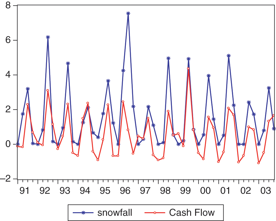
Cash Flow and Snowfall

Cash Flows of Hedging With Forwards

We first examined hedging effectiveness based on historical data. The results indicate what the effects of hedging would have been if Winter Sports had hedged its snowfall risk during the 1991-2003 period. The strike level is the average snowfall during the period. The hedge ratio is the regression coefficient of regressing cash flow on snowfall. Because of the assumptions made in Equation (2), the estimated optimal hedge ratio based on quarterly data should be the same as the one based on daily data (see Appendix B for proof).

To demonstrate the flows of cash during a forwards hedging, we list the annual snowfall, cash flow, payoffs, and hedged cash flow during the 1991-2003 period in Table 2, where the strike level is set at the average snowfall of 62.4 in.; payoff = hedge ratio × (snowfall − strike); hedged CF = unhedged CF − payoff. For example, in 1996 when the snowfall was much higher than the strike (historical average), the ski resort would have had to pay $0.47 million to the counterparty, and the cash flow would have been reduced from $2.038 to $1.566 million. In 2002, when the snowfall was lower than the strike, the counterparty would have had to pay $0.127 million to the ski resort, and the cash flow would have increased from $0.126 to $0.253 million. From the ski resort’s point of view, there are cash inflows when the snowfall is low and cash outflows when the snowfall is high. As a result, overall cash flow volatility can be reduced and remain closer to the mean.

Table 2

Flows of Cash for a Forwards Contract

Year	Snowfall	Unhedged CF	Payoff	Hedged CF
1991	50	2.681	−0.0756	2.75661
1992	71.7	4.277	0.0567	4.2203
1993	57.7	1.998	−0.0287	2.02666
1994	40.3	2.773	−0.1348	2.90775
1995	70.6	0.946	0.05	0.896
1996	139.8	2.038	0.47193	1.56607
1997	35.7	1.667	−0.1628	1.8298
1998	56.1	0.706	−0.0384	0.74441
1999	59.8	5.672	−0.0159	5.68785
2000	59.6	1.138	−0.0171	1.15507
2001	78.8	2.298	0.1	2.198
2002	41.6	0.126	−0.1268	0.25282
2003	49.5	1.399	−0.0787	1.47766
Mean	62.4	2.13223	6.3 × 10⁻¹⁷	2.13223
Variance	703.662	2.25874	0.02616	2.23258
Hedge ratio: 0.0061
Hedging effectiveness: 1.16%

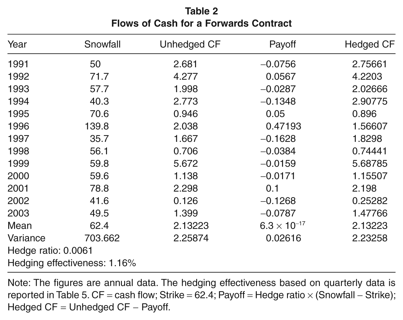
Note: The figures are annual data. The hedging effectiveness based on quarterly data is reported in Table 5. CF = cash flow; Strike = 62.4; Payoff = Hedge ratio × (Snowfall − Strike); Hedged CF = Unhedged CF − Payoff.

Monte Carlo Simulation

Under the assumption of income uncertainty, companies could produce different levels of income or cash flow even under the same conditions. Therefore, historical cash flow is considered as only one of the realizations of the random process. To test the statistical significance, the cash flow generating process has to be specified and used to simulate other possible cash flow streams. The simulation method is also well suited for this study because the basic hedging mechanisms are well defined (Graham & Smith, 1999).

To simulate the cash flows, we first had to establish the distribution of the cash flows during each period. We followed Graham and Smith (1999) and assumed the cash flow as a random walk with drift. As exhibited in Figure 1, the time series also shows strong seasonality. Seasonality can be manifested in three forms: deterministic seasonality, stationary stochastic seasonality, and nonstationary stochastic seasonality (Beaulieu & Miron, 1992). Beaulieu and Miron (1992) modeled the U.S. economic series with deterministic seasonality by arguing that (a) stochastic seasonality is not quantitatively important with the presence of seasonal dummies and (b) the source of seasonal variation in an economic series can be plausibly identified. In the present, the seasonal variation of the cash flow of a ski resort can be plausibly attributed to snowfall. We tested for deterministic seasonality in our data following the specifications in Moosa (1995) by regressing the first difference of the cash flow series on a constant and the seasonal dummies of quarters 2 to 4. All seasonal dummies are significant at the .01 level and R² is at 95.67%, indicating that the variation in cash flow accounted for by deterministic seasonality is very high. The first order difference is to eliminate the deterministic time trend, and thus, we included seasonal dummies in the model to capture the deterministic seasonality.

The cash flow generating process is eventually modeled by an AR(1) term and seasonal dummies. To examine whether this model is a proper fit for the cash flow generation process, we compared this model with three alternative specifications that capture seasonality in different ways. In Table 3, the seasonality dummies, except for the second quarter, are significant in all specifications, which indicates seasonality in the cash flow time series. In Alternative 1, we replaced AR(1) with AR(4), which is a common practice of modeling quarterly data. The AR(4), however, was not significant, and the model fit statistics of Alternative 1 all indicate a worse fit than the adopted model. In Alternative 2, we modeled the seasonality with lag terms instead of the seasonality dummies, which turn out to be the worst fit for the data. In Alternative 3, we modeled the seasonality with both dummies and lag terms. Although Alternative 3’s adjusted R² and Akaike information criterion (AIC) were better than those of the adopted model, the Scharwz criterion (SC) was not. Considering that SC punishes models with an excessive number of variables, the incremental explaining power in Alternative 3 may be because of the inclusion of more variables. Therefore, the adopted model is more parsimonious.

Table 3

Cash Flow Mean Equation Model Comparison

Variable	Adopted Model	Alternative 1	Alternative 2	Alternative 3
Constant	−0.754***	−0.733***	0.192	−0.771***
Q2	−0.149	−0.172		−0.175
Q3	3.546***	3.558***		3.562***
Q4	1.389***	1.287***		1.328***
AR(1)	0.399***		−0.050	0.322**
AR(2)			−0.064	0.318**
AR(3)			−0.039	0.055
AR(4)		0.072	0.903***	−0.135
Model fit statistics
R²	0.930	0.922	0.867	0.944
Adjusted R²	0.924	0.915	0.855	0.934
AIC	1.244	1.374	1.904	1.171
SC	1.434	1.569	2.099	1.483

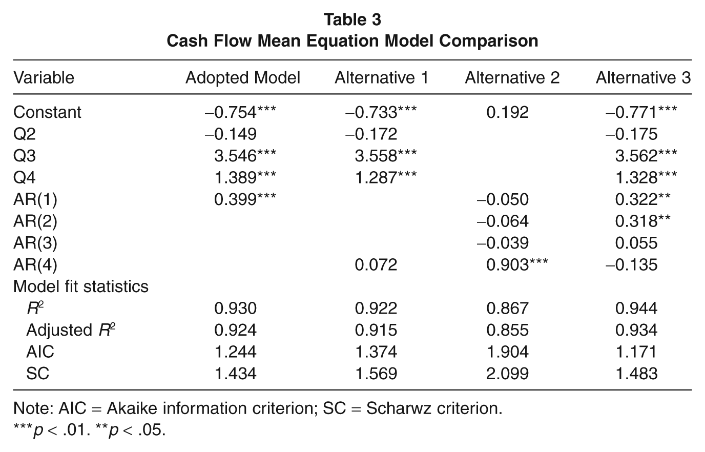
Note: AIC = Akaike information criterion; SC = Scharwz criterion.

***

p < .01. **p < .05.

For conditional means, we used historical means instead of forecasted means to maintain the correlations between simulated cash flows and historical snowfalls. To estimate variances, we adopted autoregressive conditional heteroscedasticity (ARCH) models, which specify the variance as a function of exogenous variables. ARCH models were first introduced by Engle (1982) and then generalized (GARCH) by Bollerslev (1986). We compared three simple models, ARCH(1), GARCH(1), and GARCH(1,1) for the estimation of conditional variances. ARCH(1) models the conditional variance of the error term as a function of the immediately previous error squared. GARCH(1) models the conditional variance as a function of its own lag. GARCH(1,1) is a combination of the two models. Sharing the same conditional mean equation, the three models are specified as follows.

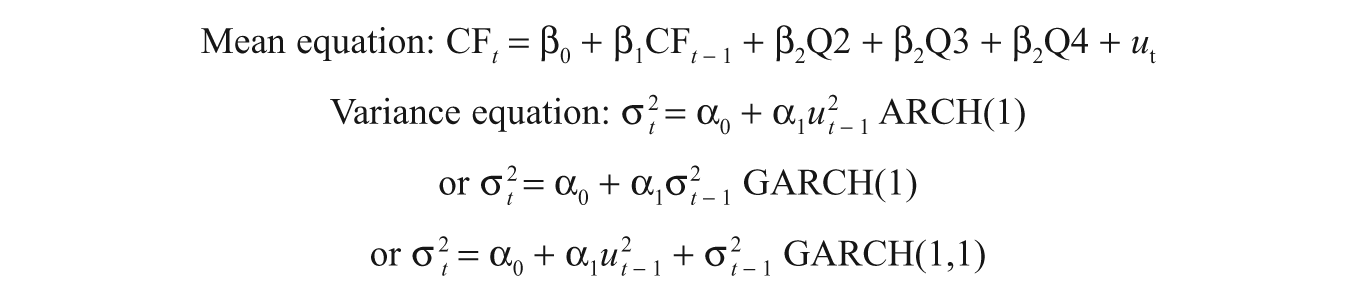
\begin{array}{l} Mean equation: C F_{t} + β_{0} + β_{1} C F_{t - 1} + β_{2} Q 2 + β_{3} Q 3 + β_{2} Q 4 + u_{t} \\ Variance equation: σ_{t}^{2} = α_{0} + α_{1} u_{t - 1}^{2} ARCH (1) \\ or σ_{t}^{2} = α_{0} + α_{1} σ_{t - 1}^{2} GARCH (1) \\ or σ_{t}^{2} = α_{0} + α_{1} u_{t - 1}^{2} + σ_{t - 1}^{2} GARCH (1, 1) \end{array}

We estimated the parameters with maximum likelihood method using EView 5.1. All three models produced satisfactory adjusted R² at around 93%. Since the GARCH(1,1) model has the smallest values of the AIC and SC, we adopted GARCH(1,1) to forecast conditional variances. The Durbin–Watson statistic of 1.86 is larger than the upper bound critical value of 1.537, indicating that the model is free of first-order autocorrelation. The estimation outputs are presented in Table 4.

Table 4

Cash Flow Mean and Variance Estimation Model GARCH(1,1)

	Coefficient	Standard Error	z Statistic	Probability
Mean equation
Constant	−0.776	0.168	−4.617	.000
Q2	−0.133	0.197	−0.676	.499
Q3	3.568	0.213	16.75	.000
Q4	1.324	0.197	6.711	.000
AR(1)	0.271	0.064	4.208	.000
Variance equation
Constant	0.152	0.271	0.561	.575
$u_{t - 1}^{2}$	−0.074	0.158	−0.470	.638
$σ_{t - 1}^{2}$	0.154	1.598	0.097	.923
R ²	0.928	Mean dependent variable		0.479
Adjusted R²	0.916	SD dependent variable		1.562
SE of regression	0.452	Akaike information criterion		1.317
Sum squared residual	8.769	Schwarz criterion		1.620
Log likelihood	−25.59	F statistic		79.274
Durbin–Watson statistic	1.862	Probability (F statistic)		0.000

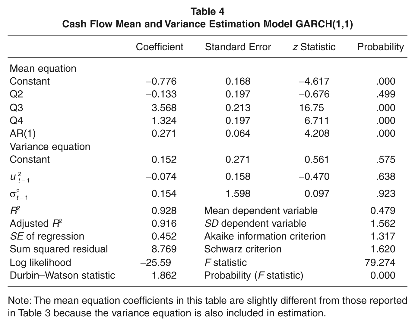
Note: The mean equation coefficients in this table are slightly different from those reported in Table 3 because the variance equation is also included in estimation.

Using the estimated means and variances as the parameters of the normal distribution, we used a random generator to simulate 1,000 quarterly and annual cash flows. We then calculated the hedging effectiveness as if snowfall forwards were applied to the simulated cash flows. With 1,000 hedging effectiveness measures for each quarter, we were able to test if the hedging effectiveness was significantly different from zero. The hedging effectiveness of snowfall forwards applied to historical and simulated cash flows is presented in Table 5.

Table 5

Hedging Effectiveness of Snowfall Index Forwards

	Q2 (September–November)		Q3 (December to–February)		Q4 (March–May)		Annual
	Historical	Simulated	Historical	Simulated	Historical	Simulated	Historical
1991–2003	64.96% (0.068)	55.79% (0.067)	1.81% (0.008)	2.78% (0.008)	0.61% (0.009)	2.29% (0.009)	1.16% (0.006)
Without 1996	23.81% (0.054)	19.26% (0.054)	30.18% (0.037)	25.80% (0.037)	8.29% (0.037)	8.47% (0.036)	6.66% (0.030)

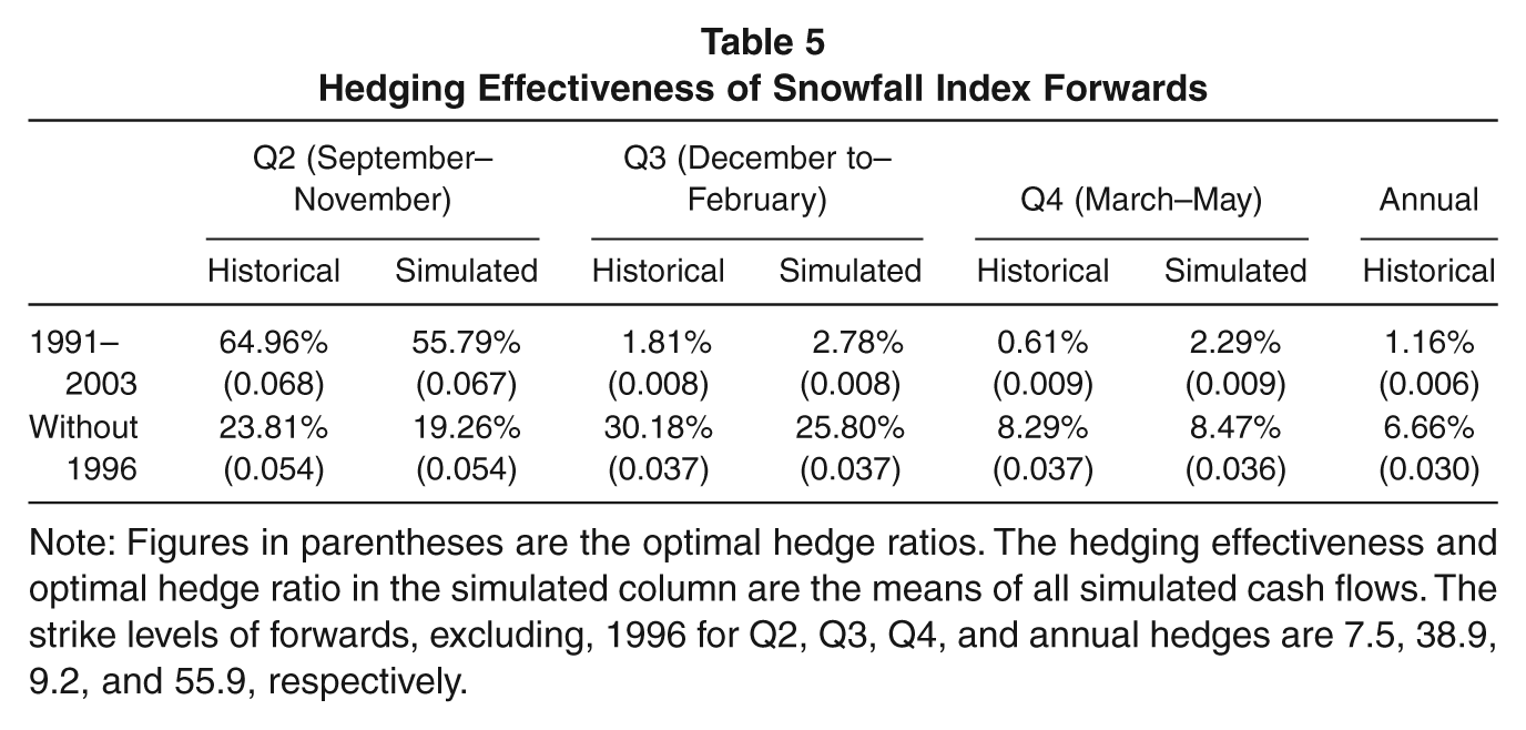
Note: Figures in parentheses are the optimal hedge ratios. The hedging effectiveness and optimal hedge ratio in the simulated column are the means of all simulated cash flows. The strike levels of forwards, excluding, 1996 for Q2, Q3, Q4, and annual hedges are 7.5, 38.9, 9.2, and 55.9, respectively.

When all years were used, the low hedging effectiveness in the third quarter clearly indicates the adverse impact of extreme snowfall, as discussed earlier. When the extreme year (1996) is excluded, hedging effectiveness is greatly improved for both historical and simulated cash flows in Q3 and Q4. Since financial hedging is designed to reduce risk due to high-probability, limited-loss events, the results that exclude 1996 are a better representation of the hedging effectiveness of weather derivatives. From a practical perspective, users of forwards contracts can benefit from imposing upper and lower limits on the payoff by avoiding the negative impact caused by extreme events. Low-probability, high-loss events, such as the case in 1996, are more appropriately managed by purchasing insurance.

Using the data excluding 1996, the hedge appears to work best in Q2 and Q3, as indicated by both historical and simulated cash flows. This is a logical outcome considering that peak snowfall and skiing activities take place during these two quarters. The results show that snowfall index forwards are indeed effective in hedging cash flow risks caused by the fluctuation of snowfalls. Such results support our proposal to reduce cash flow risk at ski resorts by using snowfall forwards. In the case of Winter Sports, the average risk exposure in Q3, the busiest quarter, is $76,479 (mean cash flow $2,067,000 × simulated mean optimal hedge ratio without 1996, 0.037). When this risk exposure is hedged by snowfall forwards, the cash flow volatility can be reduced by 25.8% on average.

Looking at the case that excludes the extreme snowfall (the row titled “without 1996”), the hedging effectiveness based on the simulated cash flows is lower than the historical cash flows for Q2 and Q3. The reason could be that the cash flows are simulated based on the random walk model, which does not incorporate the dynamic correlations between cash flows and snowfalls. In the real world, the fluctuation of cash flow is more likely to be correlated with snowfall, especially in the peak seasons. Besides technical explanations, the hedging effectiveness could be lower if part of the cash flow comes from less snow-sensitive operations, such as lodging and restaurant businesses.

Discussion

The results confirmed that snow index forwards could partly reduce cash flow volatility for ski resorts. With more stable cash flows, a company can benefit from lower tax obligations (Graham & Smith, 1999), lower bankruptcy and financial distress costs (Stulz, 2003), lower underinvestment costs (Froot et al., 1993), and, eventually, increases in firm value (Allayannis & Weston, 2001).

The results also showed that hedging effectiveness is at its best when snowfall is at its highest level. For managers, this suggests that it may not be necessary to enter a contract that covers the whole season. Hedging cash flows only for the few months that accumulate the most snowfall could be sufficient and cost effective. Extending this logic, the snowfall forwards could also be more effective for ski resorts that generate most of their cash flows through snow-related activities, such as lift ticket sales and ski schools.

Because snowfall risk is highly localized, the most efficient hedging derivatives would be the ones based on local snowfalls. For ski resorts, the ideal counterparty would be local municipalities since they have negative exposure to snowfalls because of the extra costs of paying for materials and employee overtime for cleaning streets and maintaining infrastructure. For example, in early February, 2010, mid-Atlantic cities were hit by a historic blizzard and were facing mounting bills for contractors, supplies, and equipment. Even governments with big snow cleaning budgets, such as the Virginia Department of Transportation with a $104 million budget, are operating at a deficit (Reddy & Ansberry, 2010). The budget shortfall could have been mitigated if they had entered a snowfall hedging contract with ski resorts in the vicinity.

In the case that municipalities might hesitate to enter into financial hedging positions, weather derivative brokers would be a more feasible option. These brokers buy and sell various types of weather derivatives with counterparties in various locations. Because weather risks are highly localized and not correlated with other financial risks, the brokers neutralize their risks by maintaining a diversified portfolio. The major benefit of purchasing contracts from brokers is that it reduces the expertise required. But ski resorts would have to pay fees or commissions for the service. Buying derivatives from brokers could also reduce the counterparty risk because some brokerages are divisions of big banks or insurers. For example, one of the earliest and best known weather derivative brokers, Guaranteed Weather, is a part of Mitsui Sumimoto Insurance Group. Although this study is based on a ski resort, the strategy and implementation process are also applicable to other nature-based tourism business, such as beach resorts, golf courses, and amusement parks.

We expect small individual ski resorts to benefit most from weather risk hedging because of their concentrated exposure to snowfall risk. First, individual ski resorts cannot benefit from risk reduction based on geographical diversification as ski conglomerates can. Second, smaller ski resorts usually do not have enough revenue from nonsnow activities, such as lodging, dining, or time-shares, to reduce the reliance on snow activities. Third, small resorts are usually located close to big markets and, therefore, have a higher portion of business from day visits, which could be more sensitive to snow conditions (Perdue, 2002). However, it may also be more difficult for small ski resorts to carry out financial hedging because of their lack of expertise. The bourgeoning industry of weather derivatives brokers has emerged as a provider of expertise to small businesses who are interested in weather risk hedging, but with a fee. Ski resort managers still have to decide if the benefits of hedging outweigh the costs.

This study shows that weather derivatives could reduce the cash flow volatility of nature-based tourism businesses. However, this is only the first step of studying the feasibility of applying weather risk hedging in the hospitality and tourism industry. Future studies are still needed to examine the costs and benefits associated with weather risk hedging. Another direction for future studies would be using weather derivatives to design innovative marketing programs that are otherwise not feasible. For example, a ski resort can guarantee refunds on season passes if snowfall does not exceed a desirable level. The potential losses from the refund program can be funded by the payoffs from the put options on the snowfall index. Such marketing programs could not only improve customer satisfaction by reducing customers’ risk but also increase revenue by attracting more buyers and realizing potential revenue earlier.

One of the limitations of this study is that the analysis is based on a one-property ski resort. The results might not be applicable to larger ski conglomerate that have diversified sources of income. For future studies, it would also be worthwhile to investigate the hedging effectiveness in multiproperty ski resorts or resorts with multiple lines of business. Comparisons between resorts that primarily depend on snow activities and those with diversified operations can shed some light on the effects of operational diversification on financial hedging.

Footnotes

Appendix A

Appendix B

Appendix C

References

Allayannis

Ihrig

Weston

J. P.

(2001). Exchange-rate hedging: Financial versus operational strategies. American Economic Review, 91, 391-395.

Allayannis

Weston

J. P.

(2001). The use of foreign currency derivatives and firm market value. Review of Financial Studies, 14, 243-276.

Bartram

(2001). Taking cover. Financial Management (CIMA), November, 30-32.

Beaulieu

J. J.

Miron

J. A.

(1992). A cross country comparison of seasonal cycles and business cycles. Economic Journal, 102, 772-788.

Bollerslev

(1986). Generalized autoregressive conditional heteroskedasticity. Journal of Econometrics, 31, 307-327.

Brockett

P. L.

Wang

Yang

(2005). Weather derivatives and weather risk management. Risk Management and Insurance Review, 8, 127-140.

Champion

(2008, January 23). Ski resorts tap water supply. The Wall Street Journal, p. A6.

Chicago Mercantile Exchange. (2005). An introduction to CME weather products. Chicago, IL: Author.

Chichilnisky

Heal

(1998). Managing unknown risks: The future of global reinsurance. Journal of Portfolio Management, 24(4), 85-91.

10.

Cogen

(1998). What is weather risk? Power Marketing Association Online Magazine. Retrieved from http://www.retailenergy.com/articles/weather.htm

11.

Dawkins

S. S.

Stern

(2004, June). Managing weather risk during major sporting events: The use of weather derivatives. Paper presented at the Second International Workshop on Climate, Tourism and Recreation, Crete, Greece.

12.

DeMarzo

P. M.

Duffie

(1995). Corporate incentives for hedging and hedge accounting. Review of Financial Studies, 8, 743-771.

13.

Dischel

(1999). Weather risk management: At the “Frozen Fall Fuel Company.” Retrieved from Chicago Mercantile Exchange: http://www.cme.com/files/weatherrisk.pdf

14.

Ederington

L. H.

(1979). The hedging performance of the new futures markets. Journal of Finance, 34, 157-170.

15.

Engle

R. F.

(1982). Autoregressive conditional heteroscedasticity with estimates of the variance of United Kingdom inflation. Econometrica, 50, 987-1007.

16.

Enrich

(2007). Small firms look to derivatives trading to manage costs. The Wall Street Journal, p. B4.

17.

Fairfield

P. M.

Whisenant

J. S.

Yohn

T. L.

(2003). Accrued earnings and growth: Implications for future profitability and market mispricing. Accounting Review, 78, 353-371.

18.

Froot

K. A.

Scharfstein

D. S.

Stein

J. C.

(1993). Risk management: Coordinating corporate investment and financing policies. Journal of Finance, 48, 1629-1658.

19.

Fukushima

Kureha

Ozaki

Fujimori

Harasawa

(2002). Influences of air temperature change on leisure industries: Case study on ski activities. Mitigation and Adaptation Strategies for Global Change, 7, 173-189.

20.

Gibson

(2007, April 13). Restaurant chains blame weather for falloff. The Wall Street Journal, p. C8.

21.

Graham

J. R.

Rogers

D. A.

(2002). Do firms hedge in response to tax incentives? Journal of Finance, 57, 815-839.

22.

Graham

J. R.

Smith

C. W.

(1999). Tax incentives to hedge. Journal of Finance, 54, 2241-2262.

23.

Kahl

(2008). Weather bet. Ski Area Management, 47(3), 63.

24.

Kim

Y. S.

Mathur

Nam

(2006). Is operational hedging a substitute for or a complement to financial hedging? Journal of Corporate Finance, 12, 834-853.

25.

Leggio

K. B.

(2007). Using weather derivatives to hedge precipitation exposure. Managerial Finance, 33, 246-252.

26.

Moosa

I. A.

(1995). Deterministic and stochastic seasonality in the oil imports of the Group of Seven countries. OPEC Review, 19, 181-201.

27.

Pantzalis

Simkins

B. J.

Laux

P. A.

(2001). Operational hedges and the foreign exchange exposure of U.S. multinational corporations. Journal of International Business Studies, 32, 793-812.

28.

Perdue

R. R.

(2002). Perishability, yield management, and cross-product elasticity: A case study of deep discount season passes in the Colorado ski industry. Journal of Travel Research, 41, 15-22.

29.

Petersen

M. A.

Thiagarajan

S. R.

(2000). Risk measurement and hedging: With and without derivatives. Financial Management, 29(4), 5-30.

30.

PriceWaterhouseCoopers. (2006). Weather Risk Management Association 2006 Survey results. Weather Risk Management Association. Retrieved from http://www.wrma.org/members_survey.html

31.

Quinn

L. R.

(1999). Weather derivatives begins to attract the mother of all users: Agriculture. Investment Dealers’ Digest, 65(48), 13.

32.

Reddy

Ansberry

(2010, February 9). States face big costs to dig out from blizzard. The Wall Street Journal, p. A6.

33.

Richards

T. J.

Manfredo

M. R.

Sanders

D. R.

(2004). Pricing weather derivatives. American Journal of Agricultural Economics, 86(4), 1005-1017.

34.

Scott

(2003, April). Climate change and tourism in the mountain regions of North America. Paper presented at the First International Conference on Climate Change and Tourism, Djerba, Tunisia.

35.

Scott

McBoyle

(2007). Climate change adaptation in the ski industry. Mitigation and Adaptation Strategies for Global Change, 12, 1411-1431.

36.

Scott

McBoyle

Mills

(2003). Climate change and the skiing industry in southern Ontario (Canada): Exploring the importance of snowmaking as a technical adaptation. Climate Research, 23, 171-181.

37.

Shih

Nicholls

Holecek

D. F.

(2009). Impact of weather on downhill ski lift ticket sales. Journal of Travel Research, 47, 359-372.

38.

Smith

C. W.

Stulz

R. M.

(1985). The determinants of firms’ hedging policies. Journal of Financial and Quantitative Analysis, 20, 391-405.

39.

Stulz

R. M.

(2003). Risk management and derivatives (1st ed.). Cincinnati, OH: Southwestern.

40.

Timiraos

(2007, June 8). Tribes invoke gods to block wastewater snowmaking. The Wall Street Journal, p. B1.

41.

Turvey

C. G.

(2001). Weather derivatives for specific event risks in agriculture. Review of Agricultural Economics, 23, 333-351.

42.

Weiss

L. A.

(1990). Bankruptcy resolution: Direct costs and violation of priority of claims. Journal of Financial Economics, 27, 285-314.

43.

Woodard

J. D.

Garcia

(2008). Weather derivatives, spatial aggregation, and systemic risk: Implications for reinsurance hedging. Journal of Agricultural and Resource Economics, 33, 34-51.