Conditions for Effective Application of Analysis of Symmetrically-Predicted Endogenous Subgroups

What Is the Problem?

Experimentally designed evaluations are especially good at estimating average treatment effects (the difference between mean treatment and control group outcomes), but additional questions about mediators often arise. Mediators include the experiences of sample members after random assignment that are affected by experimental group status and therefore cannot be analyzed in the same way as average treatment effects. Mediation analysis is difficult because of its endogenous nature: Being in a subgroup that is defined by a postrandom assignment experience or path is not random, and, while the effects of defined subgroups can differ, failure to recognize that a subgroup is endogenous will yield biased estimates of the effects that occurred within the subgroup.

Frangakis and Rubin (2002) provide a theoretical basis for considering the relative effects within subgroups defined by experiences that occur after randomization into an experimental evaluation. The authors frame these subgroups as strata within treatment and control groups for which within-experimental-group outcomes can be observed and compared to the potential outcomes of their counterparts in the alternative experimental group.

The evaluation of New York’s early 1990s welfare reform effort, the Child Assistance Program (CAP), provides an example of an endogenous subgroup that posed challenges for the research (Hamilton et al., 1996; Hargreaves, 1992; Peck, 2003). The reform changed the incentive structure within the welfare system (then Aid to Families with Dependent Children [AFDC]), providing more generous treatment of earnings and allowing individuals to keep more of what they earned before losing their public assistance benefits altogether. Despite the program’s generosity, just 16% of the treatment group that was offered the opportunity to enroll in CAP in lieu of being subjected to the existing welfare rules met the criteria that permitted them to be in CAP. Nevertheless, the evaluation showed substantial improvements in employment and earnings. Could those improvements have been driven by just the 16% that qualified for the alternative benefit structure? If so, then assuming no impact on the remaining 84% would have been reasonable, and the evaluation would have been justified in using a conventional Bloom (1984) correction in computing the treatment’s effects on those who took up the offer. Substantial evidence from the evaluation’s implementation study showed that the 84% of the treatment group who did not enroll in CAP still made changes in attempts to qualify: They secured new child support orders, found jobs at higher rates, and tried to meet the earnings threshold that would make CAP more attractive than AFDC (Hargreaves, 1992).

In this situation, we might wonder: To what extent did the offer of CAP motivate changes in behavior (and thereby outcomes) among those who did and did not take up the offer? Recognizing that take-up is endogenous to treatment requires extending the experimental design in new directions because (1) not only is the simple treatment-control difference insufficient to estimate the effect of take-up (2) but also comparing only those who took up the offer to the control group is inappropriate, because this method fails to account for the selection bias inherent in restricting the sample to only those within the treatment group who took up the offer.

Another example of endogenous subgroups garnering scholarly and policy attention is the Moving to Opportunity (MTO) Demonstration (e.g., U.S. Department of Housing and Urban Development, 2011). The MTO evaluation randomized public housing residents to a control group or to one of two treatment options: a voucher they could use to move anywhere or a voucher they could use only to move into a neighborhood with low poverty. Researchers were particularly interested in using the experiment to tease out “neighborhood effects,” which, in observational data, are especially hard to estimate because of the endogeneity of residential choice (i.e., families choose where to live and family characteristics, at least in part, influence family outcomes as well as neighborhood conditions). Some research has tried to capitalize on MTO’s experimental evaluation to understand the mediating effect of neighborhood quality on, for example, educational outcomes (Sanbonmatsu, Kling, Duncan, & Brooks-Gunn, 2006), health outcomes (Moulton, Peck, & Dillman, 2014), and earnings outcomes (Chetty, Hendren, & Katz, 2015). This body of research acknowledges the challenge of estimating impacts for a subgroup that arises after random assignment into a study—exposure to better neighborhood conditions—and tries to leverage the experiment to inform learning about the important policy questions.

With this as background, I now turn to a brief introduction to ASPES as a possible solution followed by specific recommendations for best practice in applying the method in the field.

How Does ASPES Address the Problem?

ASPES uses exogenous baseline characteristics to craft subgroups that are associated with some endogenous (postrandomization) choice, path, or event. In some situations, this strategy is used to overcome a missing data challenge: that some (postrandom assignment) events are defined only in either the treatment or the control group and thereby are undefined in the other. For example, the concept of take-up is a treatment group construct that is undefined in the control group. As in the CAP example above, only treatment group members had the opportunity to take up the offer of treatment, but randomization assures that they have counterparts in the control group who would have taken up the offer had it been extended to them. Because baseline characteristics are exogenous to treatment, identified subgroup impacts are internally valid. The difference in treatment and control subgroup means is an unbiased estimate of the program’s impact. As such, ASPES is a strong method for unpacking the black box: Analysts can explore what elements of a multifaceted treatment influence impact magnitude and, for example, better understand the influences of program dosage and quality. For any endogenous subgroup (such as those who took up an offer of treatment, as in CAP, or those who had long exposure to low-poverty neighborhoods in the MTO demonstration), researchers can use the approach to answer questions about whether a program’s impacts on that group are larger or smaller in magnitude (e.g., relative to those who did not take up the treatment offer or relative to those who had little or no exposure to low-poverty neighborhoods).

The basic steps for undertaking this analytic approach—where subgroups are associated with something that occurs after randomization but identified by their combination of baseline (exogenous) characteristics—are as follows:

Within a random subsample of an experimental group, use baseline characteristics to model the probability of subgroup membership within the subsample. ¹

This analytic approach involves using baseline characteristics to create subgroups, symmetrically identified in the treatment and control groups, that are associated with some postrandom assignment (endogenous) event or experience. Maintaining symmetry between the subsets of treatment and control group cases being analyzed is key to retaining the strength of the experimental design. While the general approach has been more commonly applied, two specific features of the approach—(1) using a modeling subsample that is distinct from the sample used to estimate impacts and (2) converting the results from representing impacts on predicted subgroups to impacts on actual subgroups—are unique to the ASPES approach. The first of these ensures that predicted treatment and control subgroups are symmetrical so that differences in outcomes for these subgroups are unbiased by selection or any other factors that might influence a participant’s choice to follow a given postrandomization path. The second of these means that when the required conversion assumptions are reasonable (see Bell & Peck, 2013), the converted impact estimates are also uninfluenced by selection and other sources of bias. This conversion process is necessitated by the observation that predicted subgroups do not necessarily represent the actual subgroups of interest: They are composed of a blend of individuals who are in the subgroup and those who are not. That is, while the impacts (on predicted subgroups) have internal validity, they have limited external validity. This final conversion step in ASPES involves essentially reweighting the predicted subgroups’ results by a factor that considers the correct placement rate of actuals within predicted subgroups.

The technical mechanics of the ASPES approach are beyond the scope of this article. For a better understanding of the mechanics of ASPES, the interested reader should refer to other published research (e.g., Bell & Peck, 2013; Harvill, Peck, & Bell, 2013; Peck, 2002, 2003, 2013). However, I provide a brief technical introduction here because understanding the process by which predicted subgroup results can represent the actual subgroup results is necessary for understanding some of this article’s contributions. To infer the impacts on actual subgroups, which is what we really want to know, ASPES uses two pieces of information that can be known from the data—the impacts on predicted subgroups and the proportion of actual subgroup members that is correctly placed into predicted subgroups. A conversion factor derives from the correct placement rates and is used to transform the analytic results from representing predicted to actual subgroups. ³

The ASPES approach was formally introduced into the program evaluation literature in 2003, though it has informal underpinnings in the evaluation of the Job Training Partnership Act in the early 1990s (as chronicled in Peck, 2013). Variants of the approach have been applied in a variety of settings, including in evaluating the effects of educational interventions for young children (Peck & Bell, 2014; Zhai et al., 2010; Zhai, Raver, & Jones, 2012; Zhai, Raver, & Li-Grining, 2011) and youth (Schochet & Burghardt, 2007; Unlu, Bozzi, et al., 2011; Unlu, Yamaguchi, Bernstein, & Edmunds, 2011), the effects of various aspects of welfare reforms (Gibson, 2003; Harknett, 2006; Morris & Hendra, 2009; Peck, 2005, 2007), the effects of participating in relationship counseling (Moulton, Peck, & Greeney, 2015; Wood, Moore, & Clarkwest, 2011), the effects of housing assistance (Moulton et al., 2014), and the effects of selected health and mental health interventions (Fernald, Hamad, Karlan, Ozer, & Zinman, 2008; Macias et al., 2008). In addition, the approach is the subject of active methodological exploration (e.g., Abadie, Chingos, & West, 2014; Bell & Peck, 2013; Harvill, 2013). It is routinized as part of a suite of evaluation tools called the Social Policy Impact–Pathfinder (Moulton, 2014). In addition to being used post hoc to learn more from existing experiments, the method is being built into large-scale program evaluations being carried out by the U.S. departments of Health and Human Services, Housing and Urban Development, and Labor (e.g., Peck et al., 2014).

One of these is the evaluation of the Health Profession Opportunity Grant (HPOG) program, which is funded by HHS’s ACF. In that context, the ASPES approach is being applied to a health sector–based career pathways training program targeted at recipients of Temporary Assistance for Needy Families and other low-income groups to explore what it is specifically about HPOG that drives its impacts. Considering the rich menu of trainings, education, and services that HPOG offers, the evaluation team will examine specifically whether take-up of selected program services—including, for instance, facilitated peer support groups, emergency assistance, and incentives for achieving program milestones—improves participants’ program retention and completion, and thereby their subsequent labor market outcomes. Using baseline characteristics, the analysis will identify subgroups of individuals who have selected program experiences and then analyze the effect of the program on them specifically in the spirit of delving into the black box of the HPOG program’s operations.

The next sections of this article discuss new contributions, which focus on selected practical issues that arise while carrying out ASPES.

How Strong Do First-Stage Predictions Need to Be?

The success of ASPES in identifying endogenous subgroups of interest hinges on the availability of appropriate baseline data (discussed later) and its ability to successfully predict subgroup membership. Is there a rule of thumb for what level of predictive success is “good enough” to proceed (and, when not reached, implies that ASPES should not be used)? To identify a rule of thumb answer for this question, Harvill (2014) used a simulation approach, analyzing various schemes for identifying cases in which low levels of prediction accuracy biased the estimates of impact on actual subgroups. To investigate the role of prediction accuracy, these simulations included scenarios that differed in the variance of the true value of the endogenous subgroup conditional on observations of baseline variables. When this variance is large, the baseline variables do not meaningfully distinguish between individuals in each subgroup. I refer to these cases as having low signal quality. When the variance is small, the baseline variables allow the model to meaningfully distinguish between the subgroups. This line of analysis considered whether there is a given percentage of “correct placement” threshold that flags the approach’s second-stage viability. Although statistics based on the overall prediction rate are an intuitively appealing approach to describing the performance of the prediction model, the analysis shows that such an approach does not flag cases where low signal quality biased estimates.

Instead, the analysis led to a rule of thumb that relies on the weighting factors used in the conversion step in the analysis. The simulations demonstrated that the key to obtaining consistent estimates is to limit a particular combination of the correct prediction rates away from zero. Specifically, the term [w_B + w_A − 1] must be nonzero (Note 3 shows that this is the denominator in the conversion factor). In this expression, w_B is the proportion of individuals predicted to be in Subgroup B who are actually in Subgroup B, and w_A is the proportion of individuals predicted to be in Subgroup A who are actually in Subgroup A. If this expression were precisely zero, then the conversion step could not be completed. When the term is very near zero on either side, the precision of the estimate suffers. In practice, Harvill (2014) found it sufficient to require that the absolute value of the term be greater than or equal to 0.05 as follows: |w_B + w_A − 1| ≥ 0.05.

Before applying this requirement, simulations based on specifications with high conditional variance and low signal quality produced biased estimates. Applying the requirement to all scenarios removed very few estimates that were produced by prediction models with reasonable signal-to-noise ratios and removed more than 80% of the estimates from prediction models with almost no signal. After applying the requirement, the simulation estimates closely match the true values, suggesting a substantial reduction in bias.

In practical terms, this established threshold implies that, in a given application, once the prediction stage is complete, the analyst can take the correct prediction rates, combine them together into [w_B + w_A − 1] and compute whether the result is at least 0.05 away from zero. If so, then the inputs to the analysis suggest that ASPES is appropriate to the given application. At a minimum, therefore, a correct placement rate of 52.5% in each subgroup will result in this expression equaling 0.05. This concept is related to sample size in that prediction is likely to be better in larger samples, but, as explained, it does not need to be markedly better than chance for the analysis to recover the true impacts.

What Can Be Done to Assess Sensitivity to Assumptions?

The discussion above makes mention of a specific factor that is part of the process of converting the results from representing predicted subgroups to representing actual subgroups (see Note 3). This term is computed through assumptions that must be credible in a given application to make results convincing. As elaborated elsewhere (Bell & Peck, 2013), it is preferable to have predictors that cleanly sort individuals into subgroups and that associate with impact magnitude only through that channel. From this perspective, we can think of the predicted subgroup indicator, and what goes into creating it, as being similar to an instrument: It is ideal to have predictors that associate with subgroup membership alone. On the one hand, this implies that either relatively bad (correct prediction barely better than chance) or very good (correct prediction nearing 100%) are the better conditions for the conversion assumptions to be most credible.

Although assumptions are often untestable, prior work has proposed some sensitivity analyses that can help assess the credibility of assumptions. In unpublished work that fed into an analysis of the role of Head Start center quality in influencing children’s developmental impacts (Peck & Bell, 2014), we aligned the characteristics of those in the actual quality-based subgroups that were correctly placed with the characteristics of those in the actual subgroup that were not correctly placed. In that application, there were some differences across groups in terms of their characteristics—as would be expected because these were variables used to predict subgroup membership—but those differences did not imply negating the assumption necessary to make the conversion: The impacts across these groups would be the same on average regardless of whether they are correctly or incorrectly predicted. Similarly, work on the MTO evaluation referenced earlier (see Moulton et al., 2014) revealed that, indeed, predicted subgroup members’ profiles are associated with their subsequent neighborhood experiences, but the differences between the correctly and incorrectly predicted individuals does not challenge the credibility of the underlying assumptions needed to make (and believe) the conversion. While these are two examples where examining the implications of competing profiles of characteristics led to the conclusion that the assumptions were credible, it is both feasible and likely that other applications may reach a different conclusion.

The main reason that this proposed examination of predicted and actual subgroup characteristics is recommended—as one way for assessing assumption credibility—is that we cannot actually know what the actual subgroup impacts are. Not only do we derive them only by assumption but also individuals who are in the actual subgroup are defined within only one experimental arm and undefined in the other. What we can do, however, when we cannot directly estimate the distinct subgroups’ impact, is to alleviate our concerns by examining the characteristics of each group. Are the characteristics of the actuals within different predicted subgroups really that different from one another? Although they must be to the extent that they help identify each subgroup, they might not be so distinct as to imply that their impacts should be meaningfully different. A given application will determine whether this comparison of characteristics permits the conversion assumption to pass the “gut” test.

Another option for assessing the credibility of assumptions is to use alternative assumptions to compute impacts and gauge the extent to which they report meaningfully different results. That is, with two subgroups, the necessary assumptions are fixed, but with three (or more) subgroups, a variety of assumptions is possible. Again, the Head Start quality analysis provides a useful example: The report’s appendix includes results from imposing a “preferred” set of assumptions, computes impacts using two alternative sets of assumptions, and then compares the results (Peck & Bell, 2014). In that application, varying the assumptions did not change the meaning, interpretation, or policy implications of the results. That sensitivity test led to the conclusion that the results were not assumption dependent across the range of scenarios tested. Testing the possible variation in impacts in response to varying the conversion assumptions is not based on a set logic but instead on an application-specific basis.

Future applications of ASPES should consider using one or both of these approaches: reporting the variation in subgroup characteristics according to the correct and incorrect placement of individuals and analyzing impacts based on alternative assumptions to discern the extent to which they differ meaningfully. Perhaps more importantly, future research should explore whether there is a systematized logic that might apply in testing sensitivity to assumptions. Using the first suggested approach (comparing competing profiles and seeing whether they pass the gut test regarding impact homogeneity), analysts could consider various sets of variables as inputs. Using the second suggested approach (varying assumptions to see whether that meaningfully affects estimated impacts), analysts could try a wider array of alternative assumptions than those tested in the Head Start application. These research extensions certainly would enrich the existing knowledge base.

What Types of Variables Need to Be Collected?

The main prerequisite for using ASPES is to have an experiment, but an experiment with posttest-only data is not suitable. Instead, in contrast to what is needed to calculate the average impact of an intervention, baseline data are needed to conduct any subgroup analysis and to derive impacts on endogenous subgroups. Specifically, ASPES relies on having baseline measures that can predict endogenous subgroup membership. Subgroups related to postassignment choices and events are what is generally of interest for this sort of analysis. From the control group side, these subgroups might be defined by events such as dropping out in the absence of an educational intervention, for example, or having particularly low or high earnings in the absence of a labor market intervention. From the treatment group side, these subgroups might pertain to experiencing a particularly high dosage of an intervention, experiencing a high-quality version of the program, participating in a given part of a multifaceted treatment, or achieving an intermediate treatment-related milestone. Consequently, we need to consider what corresponding individual characteristics are especially useful in predicting these kinds of endogenous choices, events, or milestones.

Evaluations often target two main sets of baseline variables: individuals’ personal, sociodemographics traits and pre-test measures of key outcomes. The first of these encompass what Shadish, Clark, and Steiner refer to as “predictors of convenience” (2008, p. 1341). Although an experimental design with randomization of units to treatment and control groups does not need to collect baseline data—a comparison of outcomes generates an internally valid estimate of the average program impact—adding baseline data permits confirming that treatment and control groups are balanced in those (measurable) ways while also allowing those variables to be used to increase precision in impact estimates by controlling for factors that, inevitably, will randomly differ between experimental groups. For the purpose of carrying out ASPES, however, less commonly collected variables, such as peoples’ motivation and preferences, are even more important because these less commonly collected variables are more useful in predicting treatment- or control-related experiences. Knowing that a participant is “motivated” to or “prefers” to participate in some aspect of a program—more so than knowing the person’s age or sex, for example—will be useful in predicting whether later he or she does participate (or alternatively, does not and drops out). Shadish et al.’s research that randomizes individuals to an experiment or into a treatment where they can self-select into their treatment option reinforces the idea that “lack of covariate richness may greatly reduce the accuracy of adjustments” in nonrandomized (e.g., propensity score) designs (2008, p. 1341).

Although the contributions of variables will depend on the specific application, here I use the National Evaluation of Welfare to Work Strategies (NEWWSs) experimental evaluation data to illustrate how three groups of variables contribute to first-stage prediction success. NEWWS involved tests of various models of welfare reform, including work- or education-focused programs, varied case management strategies, and other combinations of new program features in seven sites that operated 11 distinct programs in the 1990s (e.g., Hamilton et al., 1994). For this exercise, the endogenous subgroup is reporting being sanctioned for not complying with welfare program rules in three of the sites (a full elaboration of this topic appears in Peck, 2007). I examine three groups of variables that I designate as sociodemographic, psychosocial, and site indicators. ⁴

Sociodemographic Variables

The standard baseline variables collected by evaluations capture individuals’ demographics and some basic background traits. Table 1 lists the specific variables that the NEWWS data contain, which are the variables commonly collected in evaluations of health, social, and education programs. These variables can be used to predict sample members’ postrandomization paths, both their control group fallback choices and their treatment group program experiences. Those with younger children, for example, are more likely to take up program services such as child care; those with lower levels of education might need academic remediation as a prerequisite to job training. These variables should do at least an adequate job of predicting a broad array of postrandomization experiences. As discussed earlier with respect to prediction quality, an “adequate” job turns out to be a relatively low bar: better than chance and at least such that the term |w_B + w_A − 1| would be greater than or equal to 0.05. Any evaluation with this set of variables could consider the ASPES approach for exploring the relative effectiveness of the program on endogenously defined subgroups, but, as Shadish et al. (2008) note, additional rich variables can be quite valuable.

OPEN IN VIEWER

Table 1.

Example of Baseline Variables’ Contribution to Prediction Success.

Category of Variables	Variables Included	Indication of Prediction Success
Sociodemographic (commonly available)	Personal traits Sex (% male) Age of respondent (%): – <30 years – 30–39 years – 40+ years (omitted category) Marital status (% never married) Race and/or ethnicity (% White, % Black, non-Hispanic) Education (% with HS diploma or GED) Labor force experience (%) – Ever worked FT for 6+ months – Any earnings in past year Family traits Number of children (%): – One – Two – Three or more (omitted category) Has young child (aged 0–5 years) Public assistance (%): – Short-term recipient (receiving <2 years) – Long-term recipient (receiving 10+ years)	Significance. Of the 15 sociodemographic variables included in the prediction model, 7 are statistically significant (p < .10, 6 of which were statistically significant at the .05 level). Prediction. The percentage of observations correctly predicted is 61.8%. Conclusion. These variables alone are probably sufficient for using the ASPES approach with these data for this question (about being sanctioned).
Psychosocial (not commonly available)	Prefers FT work to parenting Prefers to stay at home with children Participation experience/likelihood/opinions (%): – Participating at baseline – Extent of barriers to participation: ■ Low (5–8) ■ Medium (9–11) ■ High (12–20) – Has problem associated with being unable to work – Has problem associated with being unable to participate – Too busy for school, training, and participation – It is unfair to make recipients work – Welfare provides better than work Psychological traits (%): – Scores high on depression scale – Feels he or she has no control over life events	Significance. Of the additional 15 psychosocial variables included in the prediction model, 6 are statistically significant (p < .10). With the added psychosocial measures in the model, the number of sociodemographic variables that are statistically significant increased from 7 to 10. Prediction. The percentage of observations correctly predicted is 71.5%. This is a marked increase of about 10% points (about a 16% relative increase). Conclusion. These variables are very valuable to identifying endogenous subgroups.
Site indicators (available in multisite evaluations)	Atlanta, GA Grand Rapids, MI Riverside, CA	Significance. Both site dummies are statistically significant and 13 of the other 30 variables are. Prediction. The percentage of observations correctly predicted increased to 75.4%.

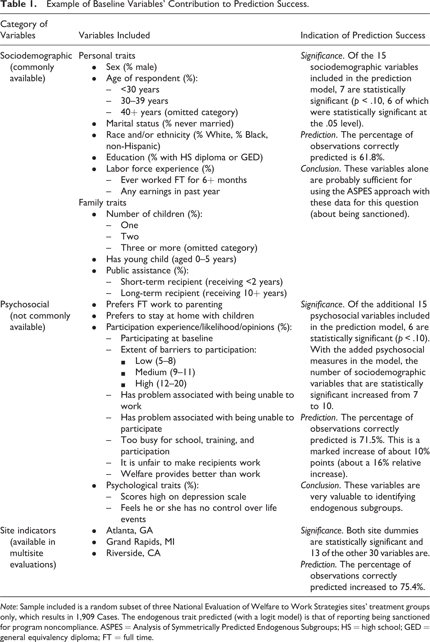
Note: Sample included is a random subset of three National Evaluation of Welfare to Work Strategies sites’ treatment groups only, which results in 1,909 Cases. The endogenous trait predicted (with a logit model) is that of reporting being sanctioned for program noncompliance. ASPES = Analysis of Symmetrically Predicted Endogenous Subgroups; HS = high school; GED = general equivalency diploma; FT = full time.

What Are the Sample Size Requirements?

The final practical consideration for effective application of ASPES that I examine here is sample size. Because there is error in each step in the analysis, ASPES-based impact estimates can be imprecise in small samples. Moulton, Peck, and Judkins (2013) derive formulas for computing the minimum detectable effects (MDEs) that can be expected from a given ASPES application. The formulas rely on several inputs, which include w_A and w_B from the discussion above. Recall that w_A is the proportion of individuals predicted to be in Subgroup A who are actually in Subgroup A, and w_B is the proportion of individuals predicted to be in Subgroup B who are actually in Subgroup B. In addition, chosen levels of power and statistical significance matter to MDEs, as does information on the treatment-control assignment ratio and the extent to which variation in outcomes can be explained by baseline variables (R ²). In analyzing some real world data from the HHS/ACF-funded HPOG program, we concluded that a sample of 804 would permit detecting impacts on a predicted subgroup equal to 0.25 standard deviations of the outcome measure but that roughly 6 times that (a sample size of 4,868) would be needed to detect the same magnitude of impacts on the actual subgroup. These conclusions rely on the assumption that the w_A and w_B are both 0.65, which we believe to be a modestly “successful” prediction rate, and one that should be achievable in a variety of circumstances. This assertion stems from observations of other applications of ASPES, where a correct prediction rate of around 65% is common. That said, these rates are higher than necessary for a given application of ASPES. The HPOG Impact Study has almost 11,000 sample members, and is, from a statistical power standpoint, a prime candidate for using ASPES to explore varied endogenous subgroups. Indeed, the project’s Evaluation Design Report (see Peck et al., 2014) flags several questions that will be pursued using this approach.

The designation of “sufficient size” is imprecise: To date very little research has considered what is “sufficient.” What we do know is that several factors serve as inputs to the conclusion about sufficient sample size: A better first-stage prediction, less noisy identification of individuals into subgroups, and greater association between subgroups and impacts all serve to reduce sample demands. For example, a shift from w_A and w_B being 0.75 (75% correct placement rate in the first stage) to w_A and w_B being 0.65 either increases the MDE by about half or imposes a roughly three-fold sample size penalty. Considering a modestly sized MDE of 0.25, the sample changes from 2,010 to 4,868 when the correct placement rates shift from 75% to 65%. For a smaller MDE of 0.15, the same prediction rate shift (from 75% to 65%) changes the sample needs from 5,586 to 13,523. Regardless of the correct placement rates, to produce impacts on a predicted subgroup requires 804 cases to detect an MDE of 0.25 and 2,233 cases for an MDE of 0.15 (S. Moulton, personal communication, November 24, 2014; Moulton, Peck, & Judkins, 2013). Larger sample sizes are needed, of course, to detect the relative difference in impacts between subgroups.

Discussion and Conclusion

This article discusses some conditions associated with the effective application of the ASPES, an analytic strategy that uses experimental evaluation data to reveal impacts on groups that form after random assignment into a study. These so-called endogenous subgroups experience various aspects of a program or achieve selected intermediate milestones; as such, they are extremely useful for helping us learn more about the relationship between the contents of a program’s black box and program impacts.

In pursuing this kind of analysis, several factors deserve special, practical consideration, as discussed in this article. Specifically, ensuring quality and appropriate baseline data will improve the first-stage prediction, which, as discussed, must be sufficient to ensure that the correct prediction rates combine to surpass a given threshold (i.e., |w_B + w_A − 1| ≥ 0.05). Related to this, any given application should assess the extent to which the necessary assumptions are appropriate, and a rich set of baseline variables can assist in that by allowing the analyst to consider the competing profiles of individuals that form the endogenous subgroups being studied. Another strategy is to run sensitivity tests, computing impacts based on more than one set of assumptions to ascertain whether the results appear to be assumption dependent. ASPES involves a first prediction stage and a final, assumption-dependent conversion stage, which together introduce error, implying that impact estimates are likely to be quite imprecisely measured in small samples. This observation leads me to the recommendation that ASPES be considered only in samples that are of sufficient size.

Of course, it would always be my preference to use design strategies to answer black box questions. Thankfully, evaluations increasingly are taking advantage of such design strategies—multiarmed or factorial designs, for example—to carve out elements of a multifaceted intervention and determine their independent and interacting effects. Lessons from these evaluations are still years away. In the meantime, we can continue to make use of rich evaluation data to learn more about which parts of those programs are responsible for impacts (or lack thereof). Further, even with more sophisticated designs, ASPES will still be a useful tool for exploring program dimensions that might not be feasible to explore in a randomized design.

This article highlights additional prescriptions for evaluation funders: Consider design and analytic innovation, invest in baseline data collection, and ensure sufficient sample size to meet analytic needs. The addition of a few strategically selected baseline characteristics beyond those commonly collected can improve the likelihood of success in applying ASPES in a given study. Further, if the ASPES approach is known to be part of a project’s analysis plan at the outset, then planning for sufficient sample size is possible.

It is my hope that future work will further explore the assumptions and inputs necessary to conducting power analyses for ASPES so that evaluators can have a clearer sense of the tradeoffs and conditions under which this analytic approach would be well applied. Also, importantly, the specific research question needs to match the evaluation design and analytic approach. For questions pertaining to posttreatment choices, events, and milestones in evaluations where we have baseline data that can be used to predict membership in those endogenous subgroups, the ASPES approach is fitting. ASPES is one of several approaches discussed in this special section that helps unpack the contents of the programmatic black box to identify how program contents are associated with program impacts. It would be helpful if future research compared these varied approaches, paying attention to the slightly different questions they each answer. Program evaluators and those managing evaluation research would certainly benefit.