Multivariate Models for Normal and Binary Responses in Intervention Studies

Abstract

Use of multivariate analysis (e.g., multivariate analysis of variance) is common when normally distributed outcomes are collected in intervention research. However, when mixed responses—a set of normal and binary outcomes—are collected, standard multivariate analyses are no longer suitable. While mixed responses are often obtained in intervention studies and analysis models that can simultaneously include such outcomes are available, we found very limited use of these models in intervention research. To encourage greater use of multivariate analysis for mixed outcomes, this article highlights the benefits and describes important features of models that can incorporate a mix of normal and binary outcomes. Models for intervention research are then fit using Mplus and results interpreted using data from an evaluation of the Early Head Start program, a randomized trial designed to improve child outcomes for an at-risk population. The models illustrated estimate treatment effects for mixed responses in standard and multilevel experimental designs.

Keywords

mixed responses multivariate analysis multilevel modeling multisite intervention

Introduction

The benefits of collecting multiple responses are well known in experimental research. First, researchers often hypothesize that a treatment impacts participants in multiple ways (e.g., increasing self-efficacy and achievement) and do not want to miss detecting important treatment effects. Second, with data on multiple outcomes, investigators can obtain a better understanding of treatment effects. For example, instead of learning that an intervention impacts wellness, researchers might find that aspects of wellness (e.g., mental well-being) are affected but not others (e.g., physical well-being). Such a finding can spur attempts to revise the intervention to enhance its effects.

While researchers often collect continuous response data (which are often presumed to be normally distributed), it is also common for investigators to collect categorical outcomes, particularly binary responses (e.g., alcohol abstinence vs. use), or more commonly a mix of continuous and categorical outcomes. For example, Wingood et al. (2011) investigated the effectiveness of a computer-based intervention for an at-risk population. They obtained outcome scores on participant knowledge (continuous) and whether or not participants reported using safe-sex practices following the intervention (binary). In addition, Berkowitz, Stover, and Marans (2011), in an intervention designed to prevent development of chronic post-traumatic stress disorder, collected outcome scores capturing symptom severity (continuous) and diagnosis (binary).

However, while mixed response data are frequently obtained in intervention studies, statistical models that simultaneously include mixed responses appear to be rarely used in these studies. To determine how often researchers use a multivariate model containing mixed responses (e.g., continuous and categorical outcomes in a multivariate model) in intervention research, we determined the type of outcome data collected based on the description of the outcomes and the analysis models used to estimate treatment effects for primary and, if applicable, secondary outcomes for all randomized experiments (N = 113) published during 2013 and 2014 in three psychology research journals: Journal of Consulting and Clinical Psychology, Health Psychology, and the Journal of Child Psychology. These journals were selected primarily because the intervention outcomes (e.g., substance abuse, nutrition and weight management, parenting, smoking cessation, stress, reading and language development, and child behavior in schools) and settings (e.g., schools, workplaces, hospitals, clinics, and via the Internet) reported in these journals are frequently encountered by evaluators and intervention researchers in general. This review suggested, first, that multivariate outcome data, as opposed to univariate, are collected and analyzed in nearly all randomized experiments (n = 110; 97%). Further, for the 110 experiments having multiple outcomes, interventions having a mix of normal and binary responses (n = 57; 52%) were more prevalent than interventions having only normal outcomes (n = 40; 36%), each of which was much more prevalent than interventions having count or categorical outcomes (n = 13; 12%). Further, while multivariate analysis models were used in most of these studies (n = 77; 70%), multivariate mixed response models were never used. That is, for the 110 randomized experimental studies where multiple outcomes were collected, the use of multivariate analysis (i.e., multivariate analysis of variance and growth curve models) was restricted to models containing a single response type (i.e., only continuous, count, or categorical outcomes), even when mixed responses were collected.

Further, methodological literature does not provide much support for investigators who wish to learn about multivariate models with mixed responses. While literature on multivariate mixed responses can be located (e.g., Browne, McCleery, Sheldon, & Pettifor, 2007; Cox & Wermuth, 1992; Olkin & Tate, 1961), the focus of this literature is not aimed at intervention research nor has it shown how investigators can apply the multivariate mixed response model to address key study objectives across commonly used experimental designs. This vacancy in the literature may explain why such models are rarely used in intervention research. Contrast that with the extensive literature on multivariate analysis models for continuous outcomes (e.g., Pituch & Stevens, 2015; Tabachnick & Fidell, 2013) as well as literature for the use of such analysis models for experimental designs specifically for psychological and educational research (e.g., Hoffman & Rovin, 2007; Tate & Pituch, 2007).

To address this gap in the literature, this tutorial paper illustrates the use of multivariate multilevel models (MVMMs) having normal and binary responses for traditional and multilevel experimental designs. We begin by reviewing the benefits associated with using MVMM. Then, we briefly describe the Early Head Start (EHS) program, an intervention that serves as the context for introducing MVMM as well as the probit link function that is used in the statistical models. After briefly describing estimation procedures associated with Mplus (Version 7.1; L. K. Muthén & Muthén, 1998–2013), we then fit models using this program, guiding the reader through examples that illustrate specification of analysis models and results interpretation. Appendix A provides Mplus code for the models fit in this article, and we also provide instructions in Appendix B for carrying out the analysis in MLwiN (Rasbash, Browne, Healy, Cameron, & Charlton, 2015). We selected these software programs because they are widely used, are among the relatively few programs capable of estimating the models described in this article, and provide manuals useful for implementing mixed model analyses. Note that while we considered using the R software program, we were unable to locate relevant documentation for the mixed responses models appearing in this article. The data set used for all analyses is found at http://www.icpsr.umich.edu/icpsrweb/ICPSR/studies/3804?q=early+head+start+research+and+evaluation+%28ehsre%29+study%2C+1996-2010%3A+[united+states]&searchSource=find-analyze-home

While this article focuses on MVMM for normal and binary responses, due to the prevalence of these response types, we note that analogous MVMMs are available for a variety of outcome types. MVMM can accommodate situations where multiple outcomes are the same type, such as all normal (Baldwin, Imel, Braithwaite, & Atkins, 2014; Goldstein, Carpenter, Kenward, & Levin, 2009; Hox, 2010; Snijders & Bosker, 2012; Tate & Pituch, 2007) or all categorical responses, the latter of which may be particularly useful when continuous outcomes deviate sharply from the assumed normality (e.g., a bimodal distribution). Note also that for moderate violations of normality, robust standard errors are available in Mplus to provide for more accurate inferences for regression coefficients. In addition, other types of mixed responses, such as responses that follow normal and categorical as well as normal and Poisson distributions, can be accommodated. MVMM can also be used to model growth across time in multiple outcomes, mixed or otherwise (Whittaker, Pituch, & McDougall, 2014). While a variety of multivariate modeling options are available, why such models are helpful relative to conducting a series of univariate analyses is an important question one might ask. We now highlight these advantages.

Advantages of Multivariate Multilevel Analysis

Several advantages are associated with the use of MVMM for mixed responses, with such advantages being similar to those for normal responses (Hox, 2010; Park, Pituch, Kim, Chung, & Dodd, 2015; Snijders & Bosker, 2012). First, tests of the effects of explanatory variables for a given response may be more powerful with MVMM than with univariate analyses. Further, this power advantage may be substantial when responses are correlated and missing outcome data are present, as MVMM does not require that participants provide scores for each response. That is, if a participant provides a score for at least one response, that participant may readily be included in the analysis. The use of MVMM, then, avoids listwise deletion of cases and the potential loss of statistical power. This power advantage is illustrated in this article with our analysis of the EHS data. Second, and relatedly, Hox notes that unlike traditional analysis approaches that assume data are missing completely at random (MCAR), the use of MVMM requires the less stringent assumption that data are missing at random (MAR). Thus, when response data are missing, Hox recommends the use of MVMM over other analyses because it provides better treatment of missing data and enables more accurate parameter estimation. Third, as we illustrate, MVMM can be used in standard experimental designs, where individuals are assigned to treatments, or in multilevel experimental designs. With multilevel designs, multiple settings are present and features of these settings may influence treatment effects. Further, when a design is multilevel, MVMM can decompose the variation and the covariation among outcomes into within- and between-cluster components. This allows an investigator to identify the degree to which correlations among responses are due to the participant or cluster level. Such information is not provided by univariate analysis. Finally, although not relevant for the mixed responses considered here, when the responses are placed on the same scale, MVMM can be used to test whether, for example, the impact of a treatment is the same or differs across the multiple outcomes. This testing procedure can be implemented for normal responses fairly easily and generally could not be implemented properly using only univariate analyses (Baldwin et al., 2014).

Research Example for Illustrative Analysis

The analyses in this article use data from the evaluation of the EHS program. Information about this intervention is available at http://doi.org/10.3886/ICPSR03804.v5. Here, we briefly describe the experimental design to provide readers a context for the analyses below. In this intervention, at each of the 17 head start centers located in different parts of the United States, low-income families with infants were randomly assigned to receive either EHS services or other community services. Thus, at each of 17 sites, a two-group randomized trial was implemented. Services provided by EHS included child development (including health, social, cognitive, and language development), parenting education, family support, and collaboration with the community to improve the quality of childcare and delivery of community services. For the 17 sites combined, the public use data set includes 2,977 families that were randomly assigned to receive EHS (n = 1,503) or control services (n = 1,474).

A variety of outcome and other measures were obtained for the evaluation across several waves. While the public use data set has many variables, a small number of variables are used here for pedagogical purposes. For the illustration, one outcome is the Bayley Mental Development Index (called hereafter MDI) collected when children were 24 months of age. The MDI is a standardized measure of child cognitive development and is one of the three Bayley Scales of Infant Development (Bayley, 1993). The second outcome, collected during parent interviews when the child was 24 months old, is a binary variable indicating whether or not the focus child was read to by the primary caregiver daily, which we refer to as read to daily, coded 1 when a child was read to daily or 0 otherwise. We also use a covariate in the first illustration below. Collected at baseline, the covariate is a binary measure of household income coded as 1 to indicate extreme poverty and 0 otherwise. Finally, group membership (EHS and control, coded as 1 and 0, respectively) was obtained following random assignment.

Table 1 shows means and standard deviations for these variables averaged across all participants for each treatment condition as well as the corresponding variable names in the public use data set. As expected due to random assignment, the control and program groups have similar levels of poverty at baseline (24% and 25%, respectively). However, at posttest, compared to control children, children receiving EHS services have a somewhat higher MDI average score and a greater proportion of such children were read to daily. Also, as is evident from Table 1, there is a substantial number of missing responses. Of the 2,977 cases, 1,726 cases have complete data for both outcomes. Thus, if listwise deletion were used, only 58% of the sample would be included in the analysis. However, a total of 448 cases that were missing data on one outcome provided data for the other. Thus, MVMM uses information from 2,174 cases (1,726 + 448) or 73%. Thus, even if the use of listwise deletion were to provide for unbiased parameter estimates, the use of MVMM, assuming the responses are correlated, will provide greater power than univariate analyses using listwise deletion, as we show below.

Table 1.

Descriptive Statistics for Each Treatment Condition.

	Control Group		Program Group^a
Measures	n	M (SD)	n	M (SD)
Bayley MDI at 24 months (B2B_MDI)^b	850	88.26 (13.53)	930	89.83 (13.79)
Child read to daily at 24 months (B2P_RD1)	1,021	0.52 (0.50)	1,099	0.58 (0.50)
Poverty (POV1)	1,474	0.24 (0.43)	1,503	0.25 (0.43)

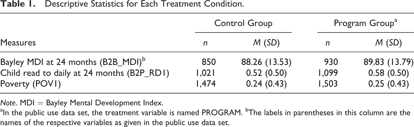
Note. MDI = Bayley Mental Development Index.

^aIn the public use data set, the treatment variable is named PROGRAM. ^bThe labels in parentheses in this column are the names of the respective variables as given in the public use data set.

The Probit Link Function

For analyses with mixed responses, the probit link function is used to transform predicted values associated with the binary outcome. Briefly, with the probit link function, a continuous variate is considered to underlie responses to the binary outcome. When this variate is scaled to have a mean of 0 and a variance (or, equivalently, standard deviation) of 1, the variate is in z-score form that then is assumed to follow a standard normal distribution.

The use of the probit function accomplishes two important things in the context of MVMM. First, the nonlinear association between the probability of Y = 1 (where Y is a binary-dependent variable) and a set of explanatory variables can be modeled. This is the case because the probabilities that can be obtained with the probit link, like the more familiar logit link, follow an S-shaped curve as a function of the explanatory variables with lower and upper asymptotes of 0 and 1, respectively. Second, the use of the probit transformation allows one to invoke the assumption of multivariate normality for the multiple outcomes, which is required for the procedure. This assumption is invoked because the z-scores that are related to the probabilities of Y = 1 are assumed to be normally distributed. As noted by Allison (2012), well-developed theory and efficient computational procedures exist for variables following a multivariate normal distribution, whereas much less is known about the multivariate logistic distribution. Simply stated, then, the use of the probit link function enables sensible estimates of effects.

Estimation Procedures

Before statistical models are presented, we comment on the estimation procedures used by Mplus for mixed response models. By default, Mplus provides weighted least squares mean- and variance-adjusted (WLSMV) estimation with the probit link function. Alternatively, maximum likelihood estimation (MLE) using adaptive numerical integration may be used with the probit link function. While WLSMV is the default estimator and generally provides for better convergence than MLE, it does not assume data are MAR but instead assumes a more restrictive missing data mechanism (referred to as MARX in Asparouhov & Muthén, 2010). When convergence is attained with MLE, it is a superior estimation method. Unlike WLSMV, MLE provides the following: maximum likelihood treatment of missing data assuming the responses are MAR, maximum likelihood estimates of parameters and associated test statistics, and statistics based on the model deviance so that the fit of various statistical models can be compared. As such, the results reported in this article use MLE with the probit link function. We note that with mixed response models Mplus also allows for maximum likelihood robust (MLR) estimation, which is MLE that yields robust estimates of standard errors, useful when continuous variables are not normally distributed. Readers interested in the details of the adaptive numerical integration estimation procedures used by Mplus may consult B. Muthén and Asparouhov (2008) and Schilling and Bock (2005).

Note that while Mplus provides model comparison statistics for mixed response models with MLE or MLR, there is no method available to test the overall fit of a single model (Bartholomew, Knott, & Moustaki, 2011), and accordingly such statistics are not provided by Mplus. However, with ML estimation, the fit of two competing mixed response models may be compared, and Mplus provides log likelihood values that allow you to form a likelihood ratio test statistic for the difference in fit between nested models (as when one or more predictors are added to a base model). Also, Mplus provides various information criteria (e.g., Bayesian) to assist in comparing the fit of competing nonnested models. Note also that when ML estimation is used with the probit link function, a factor associated with each binary outcome must be created to obtain an estimate of the residual covariance of the binary and normal outcomes. In addition, such covariances, regression coefficients, and standard errors associated with the binary outcomes need to be rescaled to provide for correspondence with probit regression results when this factor is created. Rescaling is accomplished by dividing these estimates by the square root of 2. All relevant mixed response model results reported in this article are rescaled. The Mplus code in Appendix A uses MLE with the probit link function and creates the latent factor needed for the binary outcome.

Mixed Response Models for Standard Experiments

In this section, we assume that participants have been randomly assigned to treatment conditions and are not located in different sites. We begin with this analysis to ease readers into the modeling process and because more readers are likely to have data from a nonmultilevel experimental design. A coded intervention variable is included as an explanatory variable for each outcome and a covariate is included to increase the power of the test for treatment effects. The analysis goal is to determine, compared to control children, whether children receiving EHS services have greater mean cognitive development and whether a greater proportion of such children were read to daily by their primary caregiver, after taking household poverty into account.

Equations 1 and 2 are used by Mplus for this analysis. In these equations, MDI represents the normal response and READ (read to daily) represents the binary response. These outcomes are allowed to vary and covary across participants. For each outcome, the treatment variable (program, coded 1 for EHS and 0 for control) and the poverty covariate (pov1) are included. These equations are:

MDI = β_{0} + β_{2} program + β_{4} p o v 1 + r_{0},

READ = β_{1} + β_{3} program + β_{5} p o v 1 + r_{1} .

The primary parameters of interest are β₂, which represents the difference in mean MDI scores between the treatment and the control groups, and β₃, which is the treatment effect for the parental reading variate in terms of standard deviations, with each effect holding poverty constant. Parameters β₄ and β₅ represent the association between poverty and the respective outcome, which is assumed to be the same for each treatment group. The residual terms, r ₀ and r ₁, as throughout the article, are assumed to follow a multivariate normal distribution with an expected mean of zero and constant variances and covariance. Note that the residual variance of the read-to-daily variate is set equal to 1 due to the probit link function. Also, additional covariates, as well as interaction terms (i.e., product variables), may be included, and different sets of covariates can be used in Equations 1 and 2, if desired.

Estimating Equations 1 and 2 using MLE indicates that treatment effects are present for each outcome. Table 2 shows the estimates of the regression coefficients in the mixed response column. For the MDI, the treatment effect (β₂), holding poverty constant, is 1.63 and is statistically significant (t = 2.53, p = .01). For read to daily, the treatment effect estimate (β₃) is .13 (t = 2.4, p = .02), indicating that children receiving EHS services are more likely to be read to daily than control children holding poverty constant. Holding treatment group membership constant, baseline poverty is also negatively associated with the MDI (β₄ = −2.17, t = −2.89, p < .01) but is not associated with read to daily (β₅ = −0.07, t = −1.16, p = .25). The residual variance of the MDI is 185.65 (SE = 6.22) and is fixed to 1 for read to daily. The residual covariance is 3.06 (SE = .40), which corresponds to a residual correlation among the responses of .22.

Table 2.

Regression Coefficient Estimates From the Mixed Response and Univariate Models.

Parameter	Mixed Response (n = 2,174)	Univariate (n = 1,726)
Bailey MDI
Treatment effect (β₂)	1.63* (0.65)	1.72* (0.66)
Poverty slope (β₄)	−2.17* (0.75)	−2.24* (0.77)
Read to daily^a
Treatment effect (β₃)	0.13* (0.05)	0.11 (0.06)
Poverty slope (β₅)	−0.07 (0.06)	−0.04 (0.07)

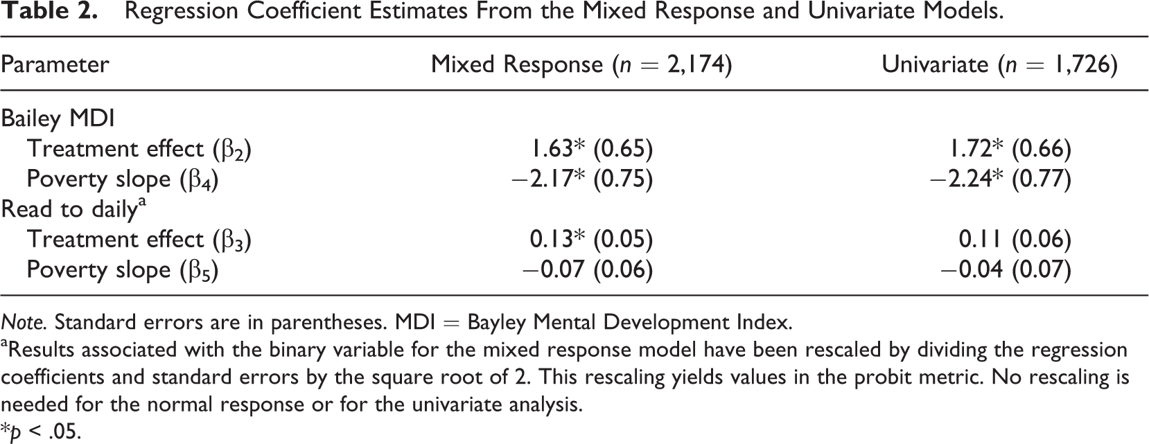
Note. Standard errors are in parentheses. MDI = Bayley Mental Development Index.

^aResults associated with the binary variable for the mixed response model have been rescaled by dividing the regression coefficients and standard errors by the square root of 2. This rescaling yields values in the probit metric. No rescaling is needed for the normal response or for the univariate analysis.

*p < .05.

Note that when we implemented listwise deletion (n = 1,726) for these same variables and estimated treatment effects with separate univariate models, the latter of which is the typical analysis approach, an important study conclusion differed. Although valid use of listwise deletion generally requires data MCAR, Allison (2002) and Enders (2010) state that use of listwise deletion will yield unbiased regression parameter estimates provided that missingness is not related to the outcome variable. That is, if missingness is related only to the predictors, including the predictors in the analysis model will yield unbiased regression parameter estimates. With our data, there is evidence supporting this condition as missingness in a given response is only related to the poverty predictor, which we include in the analysis model. However, even though the use of listwise deletion will not result in biased regression parameter estimates under this condition, use of MVMM may provide for greater power by obtaining smaller standard errors for the regression coefficients. This greater power for MVMM results from including in the analysis model (a) data from more cases and (b) the correlated multiple outcomes (Snijders & Bosker, 2012).

Bearing this out, when we estimated separate univariate regression models for each outcome using listwise deletion, we found that the point estimates of the regression coefficients in Equations 1 and 2 were generally similar to those obtained by MVMM. Inspecting Table 2, where the results of interest are shown in the univariate column, the regression estimates for the univariate analyses were sometimes larger and sometimes smaller than the corresponding MVMM estimates. However, the standard error of each regression coefficient was smaller with MVMM, and this altered an important test result for the read-to-daily variable. Specifically, a univariate probit regression model estimated for read to daily, which also included the treatment and poverty variables, indicated that this treatment effect is 0.11 (compared to the MVMM estimate of 0.13), and that the standard error of this effect is 0.06 for the univariate analysis, the latter of which is about 20% larger than the corresponding MVMM estimate of 0.05. As a result, the treatment effect estimate for read to daily is not statistically significant (p = .08) in the univariate analysis. A similar univariate logistic regression model for read to daily also did not return a significant treatment effect (b = .17, SE = .010, p = .08). This difference in analysis results between the univariate and MVMM approaches illustrates the statistical power advantage of MVMM.

Mixed Response Models for a Multilevel Experimental Design

The goal in this section is, again, to estimate treatment effects for the two outcomes. We now extend the MVMM with mixed responses to take into account that children are nested or clustered in head start centers. As is well known, such nesting, if not included in the statistical model, may violate the assumption of independence. As a result, single-level analyses that ignore such nesting may inflate the Type I error rate for tests of fixed effects. Note that investigators may encounter other situations where such clustering is present, such as clients nested within therapists, employees nested in workplaces, and pupils clustered in teachers who are nested in schools.

In this analysis, the mixed responses are included along with the treatment indicator variable. Since children are nested within centers, the multivariate model now has two levels: children (Level 1) who are nested within 1 of the 17 head start centers or sites (Level 2). The participant-level outcomes are, as before, the MDI and the read-to-daily variate. Since the treatments were administered to children within each site, the treatment indicator variable (program) is placed at the individual level of the model. This variable, initially dummy coded, is now centered within each site so that the treatment variable is uncorrelated with any site-level variable, providing for a “pure” within-site estimate of the treatment effect (see Enders & Tofighi, 2007, and Pituch & Stevens, 2015, Chapter 13, for a discussion of centering and interpretation of parameters). Thus, the multivariate Level 1 or individual-level model is:

{MDI}_{i j} = β_{0 j} + β_{2 j} {program}_{i} + r_{0 i j},

{READ}_{i j} = β_{1 j} + β_{3 j} {program}_{i} + r_{1 i j},

where the subscripts i and j represent a given individual and site, respectively. Parameters β_2j and β_3j represent the within-site treatment effects for MDI and read to daily. Parameter β_0j, as a result of the centering, represents the MDI mean for a given site j, with the residual term r _0ij capturing the child-level residual. Similarly, β_1j represents the mean z-score for the read-to-daily variate for a given site j, with r _1ij representing its within-site residual. Note that the variance of r _1ij is set to 1 due to the probit link function.

At the site level, an unconditional equation can be specified that allows the within-site means and treatment effects to vary across sites. This model is:

β_{0 j} = β_{0} + u_{0 j},

β_{1 j} = β_{1} + u_{1 j},

β_{2 j} = β_{2} + u_{2 j},

β_{3 j} = β_{3} + u_{3 j},

where β₀ and β₁ represent the overall average for the MDI and read-to-daily outcomes, respectively. The key parameters are β₂ and β₃ which represent the treatment effects averaged across sites for MDI and read to daily. The residual terms allow each of these site means and treatment effects to vary and covary. Note that if treatment effects vary across sites, they may also covary, suggesting that sites with relatively strong treatment effects on a given outcome have relatively strong effects (or weak depending on the sign of the covariance) for another outcome. When such effects vary (and covary), investigators may consider including in the model site-level variables that may predict this covariation. Investigators may include such predictors in Equations 7 and 8 to learn if a given site-level predictor (e.g., degree of treatment implementation) accounts for the observed pattern of treatment effects. Such additional analyses may be helpful in identifying variables predictive of treatment success across multiple outcomes. Note though that with a limited number of sites (17 here), estimating a relatively large number of site-level variances (4) and covariances (6) may likely result in estimation problems (e.g., lack of convergence, correlations greater than 1), especially if such population variances are small (see Bell, Morgan, Schoeneberger, Kromrey, & Ferron, 2014, for a recent discussion of these estimation issues). In fact, when we estimated Equations 3 –8, the variance estimates for the residuals in Equations 6 and 8 were 0, and for Equation 7 was 0.34 (SE = 1.90, t =1.78, p = .86). Thus, for the results reported below, only the MDI means (in Equation 5) were allowed to vary across sites.

The final model includes four fixed effects (the intercepts of Equations 5 –8) and four variance/covariance terms. These latter terms include a full covariance matrix at the child level and a site-level variance for the MDI. The results of this model are shown in Table 3. Interpreting these results, we find that children receiving EHS services score, on average, 1.54 points (p = .02) greater on the MDI than control children. For the read-to-daily variate, the treatment effect estimate is 0.13 (p = .02). Thus, children at age 24 months who received EHS services had greater cognitive development and were more likely to be read to by their primary caregiver than control children. Further, as shown in Table 3, two of the variance/covariance terms are statistically significant. That is, the MDI scores of children vary within site and the MDI and read-to-daily outcomes at the child level are positively associated (the correlation is .23), which is consistent with the notion that reading to children daily promotes cognitive development. As shown in Table 3, variation in MDI scores at the site level is not statistically significant (p = .06).

Table 3.

Maximum Likelihood Estimates for the Multilevel Mixed Response Model.

Parameter	Bayley MDI	Read to Daily^a	Covariance
Fixed effects
Mean	88.95* (0.53)	0.13* (0.03)^b
Treatment effect	1.54* (0.64)	0.13* (0.05)
Random parameters
Site level
Variance	2.96 (1.58)	—
Covariance			—
Child level
Variance	183.51* (6.18)	1
Covariance			3.09* (0.40)

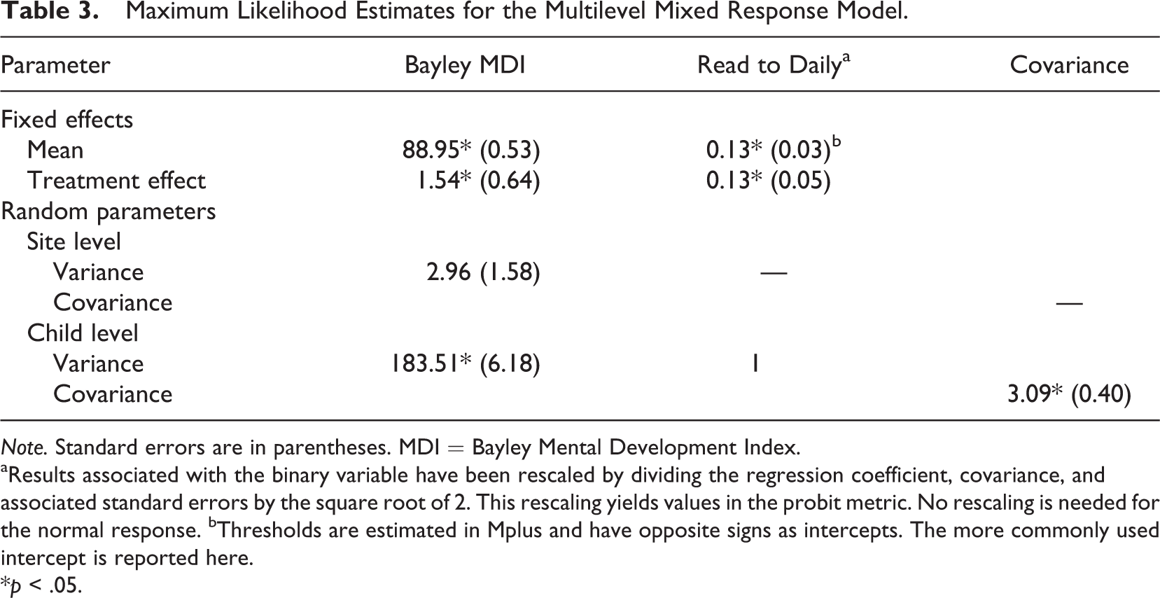
Note. Standard errors are in parentheses. MDI = Bayley Mental Development Index.

^aResults associated with the binary variable have been rescaled by dividing the regression coefficient, covariance, and associated standard errors by the square root of 2. This rescaling yields values in the probit metric. No rescaling is needed for the normal response. ^bThresholds are estimated in Mplus and have opposite signs as intercepts. The more commonly used intercept is reported here.

*p < .05.

Discussion

The purpose of this article was to introduce readers to MVMM with mixed responses in intervention research. Our intent was to demonstrate the usefulness and flexibility of this approach by showing how models can be specified to address research questions focusing on treatment effectiveness. Specifically, the models included here allow one to simultaneously test the impact of an intervention when normal and binary responses are obtained in situations where an investigator may or may not have covariates as well as assess the impact of an intervention in standard or multilevel experimental designs. As we illustrated, the MVMM approach is particularly useful, compared to separate univariate analyses, when participants have incomplete response data and/or when obtaining estimates of the response correlations are of substantive interest, particularly in multilevel designs where person-level and organization-level correlations may be obtained.

We also showed how such data can be analyzed with Mplus and illustrated the use of MVMM with data obtained from the EHS evaluation. While our examples included a two-group experimental design and two response variables, more than two groups can be accommodated in these models with additional coded treatment indicator variables, and additional responses may be included. Note though that with additional response variables, convergence issues may arise. If that is the case, researchers may need to limit the use of such models to outcomes that are at least moderately correlated, as these conditions provide for better missing data treatment and greater statistical power when missing responses occur (Snijders & Bosker, 2012).

We hope that this article encourages researchers to consider using MVMM when mixed responses are collected. As more sophisticated ways of modeling data are developed, investigators should be aware of these developments and weigh the potential contributions they have for shedding new light on empirical studies. MVMM with mixed responses is an analytic tool that is useful in a variety of situations and offers important advantages for applied researchers.

Footnotes

Appendix A

Appendix B

Declaration of Conflicting Interests

The author(s) declared no potential conflicts of interest with respect to the research, authorship, and/or publication of this article.

Funding

The author(s) received no financial support for the research, authorship, and/or publication of this article.

References

Allison

P. D.

(2002). Missing data. Thousand Oaks, CA: Sage.

Allison

P. D.

(2012). Logistic regression using SAS: Theory and application. Cary, NC: SAS Institute.

Asparouhov

Muthén

(2010). Weighted least squares estimation with missing data. Technical appendix. Los Angeles, CA: Muthén & Muthén.

Baldwin

S. A.

Imel

Z. E.

Braithwaite

S. R.

Atkins

D. C.

(2014). Analyzing multiple outcomes in clinical research using multivariate multilevel models. Journal of Consulting and Clinical Psychology, 82, 920–930.

Bartholomew

D. J.

Knott

Moustaki

(2011). Latent variable models and factor analysis: A unified approach (3rd ed.). Chichester, UK: Wiley.

Bayley

(1993). Bayley scales of infant development, Second Edition: Manual. New York, NY: The Psychological Corporation, Harcourt Brace & Company.

Bell

B. A.

Morgan

G. B.

Schoeneberger

J. A.

Kromrey

J. D.

Ferron

J. M.

(2014). How low can you go? An investigation of the influence of sample size and model complexity on point and interval estimates in two-level linear models. Methodology, 10, 1–11.

Berkowitz

S. J.

Stover

C. S.

Marans

S. R.

(2011). The child and family traumatic stress intervention: Secondary prevention for youth at risk of developing PTSD. Journal of Child Psychology and Psychiatry, 52, 676–685.

Browne

W. J.

McCleery

R. H.

Sheldon

B. C.

Pettifor

R. A.

(2007). Using cross-classified multivariate mixed response models with application to life history traits in great tits (Parus major). Statistical Modelling, 7, 217–238.

10.

Cox

D. R.

Wermuth

(1992). Response models for mixed binary and quantitative variables. Biometrika, 79, 441–461.

11.

Enders

C. K.

(2010). Applied missing data analysis. New York, NY: The Guilford Press.

12.

Enders

C. K.

Tofighi

(2007). Centering predictor variables in cross-sectional multilevel models: A new look at an old issue. Psychological Methods, 12, 121–138.

13.

Goldstein

Carpenter

Kenward

Levin

(2009). Multilevel models with multivariate mixed response types. Statistical Modelling, 9, 173–197.

14.

Hoffman

Rovine

M. J.

(2007). Multilevel models for the experimental psychologist: Foundations and illustrative examples. Behavior Research Methods, 39, 101–117.

15.

Hox

(2010). Multilevel analysis: Techniques and applications (2nd ed.). New York, NY: Routledge.

16.

Muthén

Asparouhov

(2008). Growth mixture modeling: Analysis with non-Gaussian random effects. In Fitzmaurice

Davidian

Verbeke

Molenberghs

(Eds.), Longitudinal data analysis (pp. 143–165). Boca Raton, FL: Chapman & Hall/CRC Press.

17.

Muthén

L. K.

Muthén

B. O.

(1998–2013). Mplus user’s guide (7th ed.). Los Angeles, CA: Author.

18.

Olkin

Tate

R. F.

(1961). Multivariate correlation models with mixed discrete and continuous variables. Annals of Mathematical Statistics, 32, 448–456.

19.

Park

Pituch

K. A.

Kim

Chung

Dodd

B. G.

(2015). Comparing the performance of multivariate multilevel modeling to traditional analyses with complete and incomplete data. Methodology, 11, 100–109.

20.

Pituch

K. A.

Stevens

J. P.

(2015). Applied multivariate statistics for the social sciences: Analyses with SAS and IBM's SPSS (6th ed.). New York, NY: Routledge.

21.

Rasbash

Browne

W. J.

Healy

Cameron

Charlton

(2015). MLwiN Version 2.33. Bristol, England: Centre for Multilevel Modelling, University of Bristol.

22.

Schilling

Bock

R. D.

(2005). High-dimensional maximum marginal likelihood item factor analysis by adaptive quadrature. Psychometrika, 70, 533–555.

23.

Snijders

T. A. B.

Bosker

R. J.

(2012). Multilevel analysis: An introduction to basic and advanced multilevel modeling (2nd ed.). London, England: Sage.

24.

Tabachnick

B. G.

Fidell

L. S.

(2013). Using multivariate statistics (6th ed.). Boston, MA: Pearson.

25.

Tate

R. L.

Pituch

K. A.

(2007). Multivariate hierarchical linear modeling in randomized field experiments. Journal of Experimental Education, 75, 317–337.

26.

Whittaker

T. A.

Pituch

K. A.

McDougall

G. J.

Jr (2014). Latent growth modeling with domain-specific outcomes comprised of mixed response types in intervention studies (Special Issue on Advances in Data Analytic Methods for Evaluating Treatment Outcome and Mechanisms of Change). Journal of Consulting and Clinical Psychology, 82, 746–759.

27.

Wingood

G. M.

Card

J. J.

Solomon

Braxton

Lang

… DiClemente

R. J.

(2011). Preliminary efficacy of a computer-based HIV intervention for African-American women. Psychology and Health, 26, 223–234.