Conducting Configurational Comparative Research With Qualitative Comparative Analysis

Abstract

The search for necessary and sufficient causes of some outcome of interest, referred to as configurational comparative research, has long been one of the main preoccupations of evaluation scholars and practitioners. However, only the last three decades have witnessed the evolution of a set of formal methods that are sufficiently elaborate for this purpose. In this article, I provide a hands-on tutorial for qualitative comparative analysis (QCA)—currently the most popular configurational comparative method. In drawing on a recent evaluation of patient follow-through effectiveness in Lynch syndrome tumor-screening programs, I explain the search target of QCA, introduce its core concepts, guide readers through the procedural protocol of this method, and alert them to mistakes frequently made in QCA’s use. An annotated replication file for the QCApro extension package for R accompanies this tutorial.

Keywords

configurational comparative methods (CCMs)evaluation methods qualitative comparative analysis (QCA)empirical research methods

The view of causal complexity as the multifarious interplay of necessary and sufficient conditions has long been established in many areas of evaluation research. For instance, the theory-based approach of contribution analysis assumes outcomes to result from different packages of contributory causes—alternative combinations of causes in which each cause is necessary but insufficient by itself for explaining the outcome (Mayne, 2001, 2012). Similarly, public health evaluations have made use of so-called logic models, which acknowledge the need to consider complex simultaneous pathways in the explanation of an effect (Baxter, Killoran, Kelly, & Goyder, 2010; Craig, 2013). Finally, Freedman’s (1993) necessary condition analysis aims to identify necessary conditions of success in program midlife evaluations. While the view of causal complexity in terms of combinations of necessary and sufficient conditions has been relatively widespread, formal techniques for their analysis have not been readily available. With the emergence of configurational comparative methods (CCMs) over the last two decades, the situation has changed. Researchers now have tools at their disposal that do justice to this common perspective on cause–effect relations (Thiem, Baumgartner, & Bol, 2016).

From among the family of CCMs, it has been the method of qualitative comparative analysis (QCA) in particular that has made major inroads into evaluation research (Thiem, 2014c). Balthasar (2006), for example, has studied the impact of institutional design on the use types of evaluations in the Swiss Federal Administration by means of QCA; Gross and Garvin (2011) have evaluated the effectiveness of public–private partnership contracts for toll roads in achieving their objectives; Holvoet and Dewachter (2013) have sought to identify the factors that influence the performance of national evaluation societies in low- and middle-income countries; and Pennell, Rikard, and Sanders-Rice (2014) have relied on QCA for assessing a psychoeducational fathering program developed to reduce child maltreatment in the south-eastern United States.

First proposed by U.S. political sociologist Charles Ragin in the mid-1980s (Ragin, 1987), QCA has been introduced to the evaluation community by a number of applied researchers over the last 10 years (e.g., Befani, 2013; Befani, Ledermann, & Sager, 2007; Blackman, Wistow, & Byrne, 2013; Gerrits & Verweij, 2016; Sager & Andereggen, 2012; Verweij & Gerrits, 2013). Yet, among these expository primers, a hands-on tutorial that incorporates the latest methodological advances is still missing. I fill this gap with the present article, which has three primary objectives: first, to create a thorough understanding of the search target of QCA; second, to guide readers through the method’s procedural protocol; and third, to alert current and prospective users to consequential mistakes still frequently made in QCA’s use. To this end, I revisit a recent evaluation of patient follow-through effectiveness in Lynch syndrome tumor-screening programs by Cragun et al. (2014). These authors have not only relied on QCA to produce meaningful results, but they have also reflected on the perceived utility of this method for answering questions arising in evaluations of health-care provision measures in a separate article (Cragun et al., 2016).

So as to allow readers to perform this reanalysis themselves, an annotated replication file for the QCApro extension package for the R environment accompanies this tutorial (Thiem, 2016b).¹ This file also includes additional material and may be used as an adaptable template for readers’ own research. Last but not least, important concepts of configurational comparative research with QCA are put in italic font-style at their first occurrence in the text in order to provide further orientation for newcomers to CCMs in general, and QCA in particular.²

Epistemological Foundations and the Search Target of QCA

Although QCA has been used by social scientists for about one quarter century now, its epistemological foundations remain, surprisingly, largely unknown. While it is undisputed that the purpose of QCA is causal inference on the basis of regularity-theoretic relations of necessity and sufficiency (Ragin, 1987, pp. 19–33; Rihoux, 2006, p. 682; Schneider & Wagemann, 2012, p. 8), it has recently been demonstrated that the theory of causality underlying QCA and its associated Boolean-algebraic machinery have not been fully understood, with detrimental consequences for the validity of numerous results presented in applied and methodological research over the last 25 years (Baumgartner, 2015; Baumgartner & Thiem, 2015b, 2015c; Cooper & Glaesser, 2016; Thiem, 2014b, 2014c, 2016a; Thiem & Baumgartner, 2016a, 2016c; Thiem, Baumgartner, et al. 2016). It is thus important to first clarify the epistemological underpinnings and the search target of QCA.

QCA firmly rests on the theory of INUS causation, which has been most prominently associated with the writings of John L. Mackie (1965, 1974), and which can be traced back at least to John S. Mill’s concept of “chemical causation” and his methods of agreement and difference.³ Conceptually, an INUS condition is an insufficient but necessary part of a condition which is itself unnecessary but sufficient for an outcome. The meaning of this at first glance somewhat cryptic term becomes clear during the following illustration, which is deliberately based on an everyday example for reasons of easy accessibility to as wide a readership as possible.

Imagine a fire brigade to have arrived just in time to save a house from being burned to the ground. After an investigation has been concluded, it is agreed, informed by many years of experience with similar cases, that a short circuit was the cause of the fire. What is meant therewith? It is not meant that the short circuit was a necessary condition of the fire because an arson attack could have led to the same result. Nor is it meant that the short circuit was a sufficient condition of the fire. In the presence of a sprinkler, or the absence of flammable material, the short circuit would not have led to the outbreak of the fire. Without the short circuit, however, the absence of a sprinkler and the presence of flammable material would not have caused the fire, either. The short circuit was thus neither necessary nor sufficient for the fire, but indispensable in leading to its outbreak in combination with the other two conditions. Put differently, the short circuit was an insufficient but necessary part of a combination of other individually insufficient but necessary conditions of the fire. The goal of QCA is to identify such causal paths, that is, groupings of conditions or events that are difference makers to an outcome.⁴

More formally, let the presence of a short circuit be denoted by SC, the presence of flammable material by FM, the presence of a sprinkler by SP, an arson attack by AA, the fact of a house being less than 10 miles away from the fire brigade buildings by FBB, and the outbreak of a fire by OF. Then, the fire authorities might find, after a 5-year monitoring study with data on all houses in a town, a verbalized QCA model such as m ₁ in Expression 1:

m_{1} : If, and only if, S C and F M and not S P, or F M and not S P and A A and not F B B, then O F .

In QCA symbolism, which mainly draws on the syntax of propositional logic, m ₁ is usually written as m _1* in Expression 2:

\begin{matrix} (i) & (ii) \\ m_{1 *} : & (S C \land F M \land \neg S P) \lor (F M \land \neg S P \land A A \land \neg F B B) \leftrightarrow O F \end{matrix}

where “∧” denotes the AND operator, “¬” denotes the NOT operator, “∨” denotes the OR operator, and “↔” denotes the equivalence operator. Equivalence means that the expression to the left side of the double arrow—the antecedent—is necessary and sufficient for the expression to the right side—the consequent.⁵ If the antecedent is not necessary for the consequent, the implication operator, “→”, is used instead. An expression whose main operator is the AND operator is called a conjunction; one whose main operator is the OR operator is called a disjunction. Paths (i) and (ii) are each conjunctions, whereas the antecedent in m _1* is a disjunction.

Put in plain English, in this 5-year monitoring study, two alternative causal paths have been identified: a fire breaks out in a house when (i) a short circuit, and the presence of flammable material, and the absence of a sprinkler occur together, or when (ii) flammable material, and the absence of a sprinkler, and an arson attack, and the fact of the respective house being at least 10 miles away from the fire brigade buildings occur together.

It is important to recognize that m _1* is not declared by QCA to be representing the entire causal story behind the outbreak of fires in houses. This model merely claims that there exist at least two causal paths to the outbreak of a fire in a house (implying “and possibly additional causal paths”), each of which features at least those conditions (implying “and possibly additional conditions”) identified in m _1*.⁶

But how does QCA ensure that what it outputs is causally interpretable in this way in the first place? The process whereby QCA models are rendered causally interpretable in accordance with the INUS theory of causation is called minimization. In minimization, a custom-built algorithm eliminates redundancies (cf. Duşa & Thiem, 2015; Thiem, 2015a; Thiem & Duşa, 2013a). For instance, in Path (i), an arson attack is redundant because a fire breaks out irrespective of whether this condition is present or absent, just as in Path (ii) a short circuit is. As short circuits have been observed at any distance from the fire brigade’s buildings in contrast to arson attacks (possibly because arsonists do not want the fire brigade to arrive in time), the latter is also a redundant condition in Path (i).

Although rigorous minimization is of the essence, even prominent methodologists have not been cognizant of this basic requisite of using QCA for purposes of causal inference. For instance, Schneider and Wagemann (2012, p. 108) tell their readers that ¬A ∨ A¬BC → Y is an acceptable QCA solution because “A can indeed be a causally relevant INUS condition for Y.” This is erroneous. Simple transformations prove A to be a redundant conjunct in A¬BC, meaning that A cannot be an INUS condition (see Thiem & Baumgartner, 2016a, p. 805, fn. 6). Only those conditions that survive unconstrained minimization are causally interpretable (cf. Baumgartner, 2015).

With the search target of QCA now clarified, I proceed to explain the work flow of the method in more detail in the following section. I illustrate each step by revisiting Cragun et al. (2014). In this study, the authors analyze the association between different universal tumor-screening procedures and certain levels of patient follow-through with germ-line testing for Lynch Syndrome after a screen-positive result, using web-based survey and telephone interview data obtained from 15 U.S. Lynch Syndrome Screening Network institutions.

The Procedural Protocol of QCA

The procedural protocol of QCA, as visualized in Figure 1, can be divided into three phases (cf. Baumgartner & Thiem, 2015a, 2015b; Thiem, Spöhel, & Duşa, 2016, p. 108): the transformation of raw data into a truth table (Phase I), the minimization of the function described by the truth table to a prime implicant (PI) chart in the first algorithmic stage (Phase II), and the decomposition of this chart for deriving the solution in the second algorithmic stage (Phase III). The researcher has maximum control over Phase I, whereas no direct control can be exercised over Phases II and III, which are hardwired in the minimization algorithm.

Figure 1.

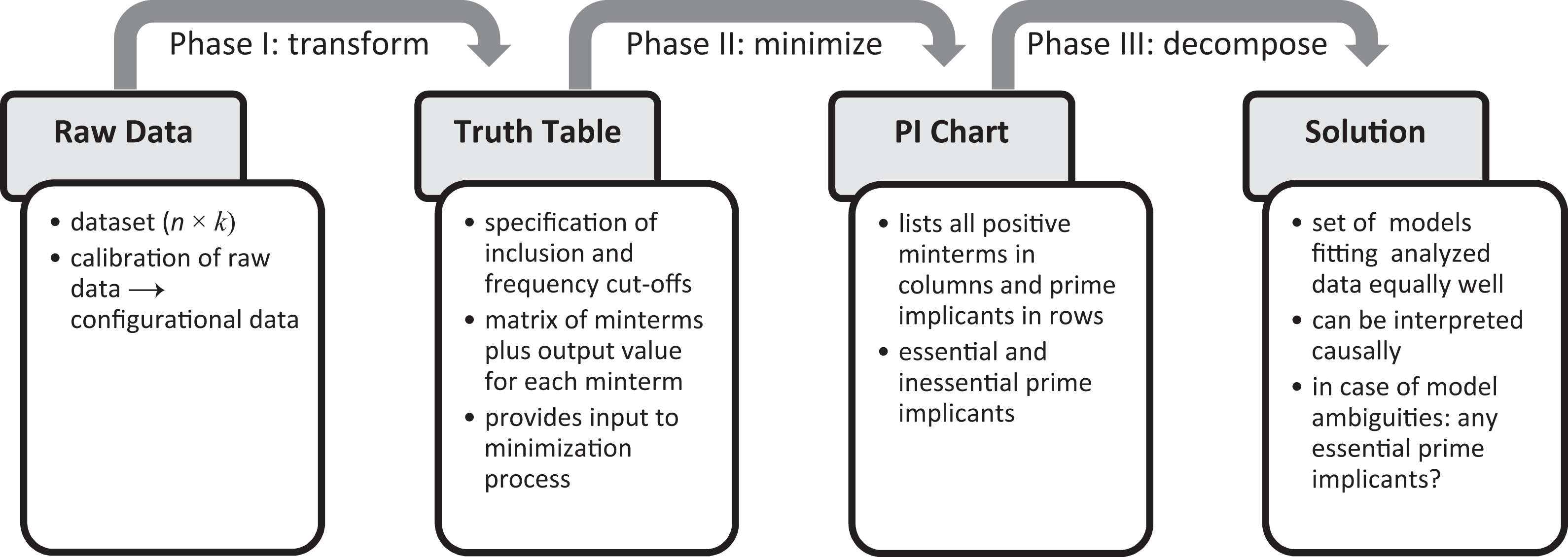
Procedural protocol of qualitative comparative analysis.

Phase I: From the Raw Data to the Truth Table

Similar to the requirements of other formal methods of causal data analysis, the main input to QCA is a data set of dimension n × k, with n being the number of cases (rows) and k the number of variables (columns). These data are called raw data. Specific to QCA is that raw data first have to be calibrated, whereby variables are transformed into factors, that is, categorical variables whose levels provide the basis for sets of interest. Once this process has been completed, the new data are referred to as configurational data. These data are subsequently divided into a set of exogenous factors and one endogenous factor, from the latter of which the outcome to be analyzed is selected. The set of all factors included in a QCA run, both exogenous and endogenous, is referred to as the factor frame.

The raw and configurational data for the study by Cragun et al. (2014) are presented in Table 1. The raw endogenous variable measures the approximate percentage of patients with a screen-positive result who have pursued germ-line testing (pf). Six binary variables are hypothesized to be causally relevant for achieving certain percentage ranges in germ-line testing: whether the challenges to the adoption of universal tumor screening have been at least as numerous as the facilitating conditions (CA; 1: yes, 0: no), whether automatic reflex testing of screen-positive tumors has been in place (AR; 1: yes, 0: no), whether a genetic counselor has received screen-positive results (RR; 1: yes, 0: no), whether a genetic counselor has disclosed screening results to patients (DR; 1: yes, 0: no), whether there have been difficulties in contacting patients (DC; 1: yes, 0: no), and whether the need for a physician referral has been a barrier (PR; 1: yes, 0: no).

Table 1.

Data Set on 15 Lynch Syndrome Screening Network Institutions in the United States Analyzed by Cragun et al. (2014).

	Raw Data
		Configurational Data
	Endogenous Variable	Exogenous Variables/Factors						Endogenous Factors (Calibrated)
Case	pf (%)	CA	AR	RR	DR	DC	PR	HPF	LPF	PF
1	>85	0	1	1	1	0	0	1	0	2
2	71–85	0	1	1	1	0	0	1	0	2
3	56–70	0	1	1	1	0	0	1	0	2
4	41–55	0	1	1	1	0	0	1	0	2
5	41–55	1	1	1	1	0	0	1	0	2
6	26–40	0	0	1	1	1	0	0	0	1
7	26–40	0	1	1	0	1	1	0	0	1
8	26–40	0	0	1	1	1	0	0	0	1
9	26–40	0	1	1	0	0	1	0	0	1
10	11–25	0	1	1	0	0	1	0	0	1
11	≤10	1	0	1	0	0	1	0	1	0
12	≤10	1	0	1	0	0	1	0	1	0
13	≤10	1	1	1	0	0	1	0	1	0
14	≤10	0	1	0	0	0	1	0	1	0
15	≤10	0	0	0	0	0	1	0	1	0

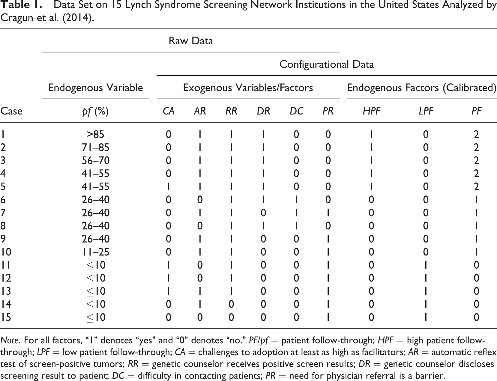
Note. For all factors, “1” denotes “yes” and “0” denotes “no.” PF/pf = patient follow-through; HPF = high patient follow-through; LPF = low patient follow-through; CA = challenges to adoption at least as high as facilitators; AR = automatic reflex test of screen-positive tumors; RR = genetic counselor receives positive screen results; DR = genetic counselor discloses screening result to patient; DC = difficulty in contacting patients; PR = need for physician referral is a barrier.

In their study, Cragun et al. (2014) calibrated the data on their endogenous variable pf with seven values (1: ≤ 10%; 2: 11–25%,…, 7: > 85%) to obtain two bivalent endogenous factors, one labeled “high patient follow-through” (HPF), the other “low patient follow-through” (LPF). Those institutions that had a high pf score (> 40%), those with a low pf score (≤ 10%), respectively, were assigned the Level 1 on HPF, LPF, respectively. Institutions with a medium score were of no direct interest to the authors.⁷

When variables are already categorical, calibration is not necessary unless the informational content of the available data should be reduced by grouping categories together for analytical purposes, as has been the case for Cragun et al. (2014), or computational reasons. This is why none of the exogenous variables CA to PR needed to be calibrated separately; they already corresponded to calibrated factors. However, when variables are continuous, some sort of transformation via a specific membership function that maps the variable onto a target set is necessary because the categorization of each unique value of a continuous variable would lead to the explosion of the dimension of the truth table—the central device in Phase I of QCA to which we now turn.⁸

A truth table is a matrix of all minterms derivable from the set of exogenous factors. Minterms are unique conjunctions of as many simple conditions as there are exogenous factors in the factor frame, with each condition representing one level of one exogenous factor such that no exogenous factor occurs twice. For example, the conjunction of challenges to the adoption of universal tumor screening having been at least as numerous as the facilitating conditions, automatic reflex tests of screen-positive tumors having been in place, a genetic counselor having received positive screen results, a genetic counselor having disclosed screening results to patients, the presence of difficulties in contacting patients, and the need for a physician referral having been a barrier represents one minterm. As Cragun et al. (2014) analyze six bivalent exogenous factors, there are 2⁶ = 64 minterms.

A matrix of minterms is not enough to constitute a QCA truth table. Still missing is a column of output values, which provide important information to the minimization algorithm in Phase II. These output values are derived in Phase I on the basis of two parameters: the inclusion cutoff (also called consistency cutoff) and the frequency cutoff.

The inclusion cutoff specifies the lower bound for the share of cases that show the outcome in relation to all cases that exhibit the same minterm. The frequency cutoff sets a lower limit for the absolute number of cases within a minterm for this minterm not to be classified as a remainder. As remainders are treated as unobserved conjunctions of conditions, they receive an output value of “?”. If a minterm meets the frequency cutoff but not the inclusion cutoff, it is classified as negative and receives an output value of “0”. And if a minterm meets the frequency cutoff as well as the inclusion cutoff, it is classified as positive and receives an output value of “1”.

The truth table that results from the data presented in Table 1 and the parameter decisions taken by Cragun et al. (2014) is given in Table 2, where the first column “Minterm” specifies the minterm index number, the following six columns from “CA” to “PR” the exogenous factors, the column “OUT” the output value, the column “INCL” the inclusion score, the column “n” the number of cases from Table 1 that conform to the respective minterm, and the column “Cases” those cases that instantiate the respective minterm. As there are no cases in Table 1 that instantiate the same minterm yet exhibit a different level on the endogenous factor, inclusion scores are equal to output values.⁹

Table 2.

Truth Table for Configurational Data in Table 1.

Minterm							OUT		INCL
Minterm	CA	AR	RR	DR	DC	PR	HPF	LPF	HPF	LPF	n	Cases
2	0	0	0	0	0	1	0	1	0.00	1.00	1	15
15	0	0	1	1	1	0	0	0	0.00	0.00	2	6, 8
18	0	1	0	0	0	1	0	1	0.00	1.00	1	14
26	0	1	1	0	0	1	0	0	0.00	0.00	2	9, 10
28	0	1	1	0	1	1	0	0	0.00	0.00	1	7
29	0	1	1	1	0	0	1	0	1.00	0.00	4	1, 2, 3, 4
42	1	0	1	0	0	1	0	1	0.00	1.00	2	11, 12
58	1	1	1	0	0	1	0	1	0.00	1.00	1	13
61	1	1	1	1	0	0	1	0	1.00	0.00	1	5
.	.	.	.	.	.	.	?	?	—	—	—	—

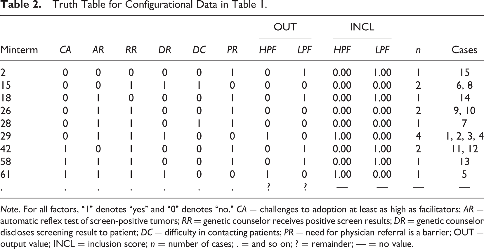
Note. For all factors, “1” denotes “yes” and “0” denotes “no.” CA = challenges to adoption at least as high as facilitators; AR = automatic reflex test of screen-positive tumors; RR = genetic counselor receives positive screen results; DR = genetic counselor discloses screening result to patient; DC = difficulty in contacting patients; PR = need for physician referral is a barrier; OUT = output value; INCL = inclusion score; n = number of cases; . = and so on; ? = remainder; — = no value.

For example, Minterm 29 is instantiated by four cases, namely 1, 2, 3, and 4. None of these Lynch Syndrome Screening Network institutions shows a low patient follow-through rate, as a result of which the inclusion score of this minterm is 1, and its output value is 1. Therefore, Minterm 29 is positive. However, had Cragun et al. (2014) set an inclusion cutoff of .8, and had Case 4 had a low patient follow-through rate, then the inclusion score of Minterm 29 would have been 3/4 = .75, which is lower than .8, and Minterm 29 would have received an output value of 0, turning it into a negative minterm.

In the form of Table 2, a truth table is suitable for minimization in Phase II of QCA. Before I go into the details of this phase, one of the most persistent misconceptions in connection with Phase I shall be dispelled, namely, that QCA is a method designed for the analysis of only small-to-moderate numbers of cases (see, e.g., Balthasar, 2006, p. 362; Befani et al., 2007, p. 175; Sager & Andereggen, 2012, p. 65; Verweij & Gerrits, 2013, p. 46). As Cragun et al. correctly argue, “QCA […] can be used to analyze small, medium, and large data sets” (2016, p. 269), the reason being that, irrespective of how many cases a data set has, data can always be transformed into a truth table once it is calibrated. For evaluation scholars and practitioners working with large data sets, QCA is no less an option than for those who analyze small data sets. By extension, case numbers are no justification for the use of QCA in lieu of other formalized methods of causal inference (Thiem, 2014c).

Phase II: From the Truth Table to the PI Chart

First, a little bit more about the different variants of QCA must be known because “QCA” has started to become an umbrella term for a family of different analytical variants since the introduction of fuzzy sets by Ragin (2000). The structure of the calibrated data under the factor frame determines the variant, four of which presently exist (Thiem, 2014d): crisp-set QCA (csQCA), fuzzy-set QCA (fsQCA), multi-value QCA (mvQCA), and generalized-set QCA (gsQCA). While gsQCA is still relatively novel and has not yet been employed, the other three variants have already been used in empirical research.¹⁰

The main difference between fsQCA and csQCA is that the former uses fuzzy sets, for which set membership is graded numerically between 0 and 1, unlike the latter, which uses crisp sets, for which set membership is determined dichotomously by “in” and “out” states (Zadeh, 1965). However, as QCA cannot operate on continuous variables, both fsQCA and csQCA currently implement the same minimization logic, in which truth tables are built on the basis of bivalent factors.¹¹ The difference between mvQCA and csQCA is that the former is employed with numbers of factor levels larger than 2. If all factors are bivalent, mvQCA reduces to csQCA. All of the variables in the raw data analyzed by Cragun et al. (2014) are calibrated as bivalent crisp-set factors, hence the use of csQCA in this study.¹²

Once the appropriate QCA variant has been chosen and all output values have been determined to complete the truth table, the identification of PIs begins, which is the technical term for potentially causal paths such as (i) and (ii) of m _1* in Expression 2. It has already been noted that this identification process consists in the elimination of redundant conditions. Various algorithms have been proposed to this end, each with its strengths and weaknesses, but algorithmic details are of no direct importance in this tutorial. What is worth being reiterated is that all redundancies—that is, nondifference-making factors—must be eliminated if the goal is to infer causally interpretable models.

The PI charts for both HPF and LPF, respectively, are presented in Table 3, where the positive minterms from Table 2 are listed across the columns, and the PIs down the rows. A cross at the intersection of a PI and a positive minterm indicates that this PI covers the minterm, a dash that this PI does not cover the minterm.

Table 3.

Prime Implicant Charts for High and Low Patient Follow-Through.

	HPF			LPF
	Minterms			Minterms
Prime Implicants	29	61	Prime Implicants	2	18	42	58
AR ∧ DR	×	×	¬RR	×	×	—	—
AR ∧ ¬PR	×	×	¬AR ∧ ¬DC	×	—	×	—
CA ∧ ¬DR	—	×	¬AR ∧ ¬DR	×	—	×	—
CA ∧ ¬PR	—	×	¬AR ∧ ¬PR	×	—	×	—
¬DC ∧ ¬PR	×	×	CA ∧ ¬AR	—	—	×	—
DR ∧ ¬DC	×	×	CA ∧ ¬DR	—	—	×	×
			CA ∧ ¬PR	—	—	×	×

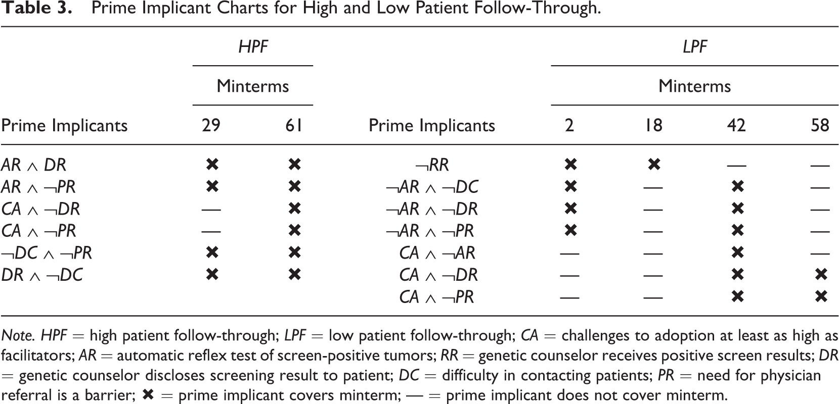
Note. HPF = high patient follow-through; LPF = low patient follow-through; CA = challenges to adoption at least as high as facilitators; AR = automatic reflex test of screen-positive tumors; RR = genetic counselor receives positive screen results; DR = genetic counselor discloses screening result to patient; DC = difficulty in contacting patients; PR = need for physician referral is a barrier; × = prime implicant covers minterm; — = prime implicant does not cover minterm.

The PI chart for HPF contains six PIs, whereas the PI chart for LPF contains seven PIs. These are all potential causal paths for which there is evidence in the data presented in Table 1. The derivation of the PI chart concludes Phase II.

As before, a mistake often made in QCA research shall be broached at the end of this subsection. A problem in connection with Phase II results from a misunderstanding of QCA’s search target and the definition of necessary conditions. Ragin (2000, pp. 254–255) as well as Schneider and Wagemann (2012, pp. 197–219), for example, have strongly recommended testing for simple necessary conditions prior to minimization in order to prevent their potential elimination during minimization in Phase II. Applied evaluation researchers have tended to follow these recommendations more or less coherently (Holvoet & Dewachter, 2013; Ledermann, 2012; Ozegowski, 2013; Pattyn & Brans, 2015; Thygeson et al., 2012).¹³ However, isolated tests for simple necessary conditions prior to minimization are fallacious. Such tests are based on an overinflation of the Boolean definition of necessity with a causal interpretation, which has its roots in the misguided belief that “X ₁ is a necessary cause of Y ₁ if Y ₁ is a subset of X ₁” (Mahoney, Kimball, & Koivu, 2009, p. 118). The formal definition of the Boolean-algebraic operation of implication underlying every relation of necessity, X ₁ ← Y ₁ ≡ X ₁ ∨ ¬Y ₁ ≡ ¬[¬X ₁ Y ₁], does not entail that X ₁ is a cause of Y ₁ (Thiem & Baumgartner, 2016a; Thiem, Baumgartner, et al., 2016). The mere necessity of a simple condition for an outcome does not perforce make it causally interpretable in accordance with the INUS theory of causation underlying QCA.

Cragun et al. (2014) were correct in not implementing such tests for simple necessary conditions to constrain Phase II of QCA, but Cragun et al. (2016) argue that they did not perform such tests in their original study because they had no hypotheses about necessary conditions. Had they strictly followed Ragin’s and Schneider and Wagemann’s guidelines and tested for necessary conditions, they would have found 6 of them for HPF and 11 for LPF (at an inclusion cutoff of .8). Among the six conditions for HPF is also RR. Yet, as the PI chart in Table 3 reveals, RR is no INUS condition for HPF. Forcing QCA to output RR as causally relevant nonetheless amounts to an invalidation of the epistemological and algebraic foundations on which the method is built. Evaluators using QCA should therefore never perform isolated tests for necessity in the context of causal data analysis with QCA (Thiem, 2014c, 2016c).

Phase III: From the PI Chart to the Solution

When all PIs have been identified at the end of Phase II, the next stage of QCA in its search for causally interpretable models is the decomposition of the PI chart in Phase III. It is only here that QCA searches for causally interpretable necessary conditions (Thiem & Baumgartner, 2016a, p. 803). This process consists in finding all disjunctions of PIs that minimally cover all positive minterms, that is, disjunctions which contain no redundant PIs. As in Phase II, this process is hardwired in the respective minimization algorithm implemented in the software that is used by the researcher (Thiem, 2015b).

In their study, Cragun et al. (2014) present a QCA solution with exactly one model for high patient follow-through, and a QCA solution with exactly one model for low patient follow-through. These two models are restated as m_HPF and m_LPF in Expressions 3 and 4:

m_{H P F} : A R \land D R \land \neg D C \land \neg P R \leftrightarrow H P F,

m_{L P F} : \neg D R \land C A \lor \neg R R \leftrightarrow L P F .

The authors believe to have found that the combination of automatic reflex testing and the disclosure of screen-positive results and the absence of major barriers in contacting patients and the absence of barriers in obtaining a referral from a physician accounts for the achievement of high patient follow-through rates. At first sight, this explanation sounds convincing. At second sight, however, the PI chart for HPF in Table 3 reveals that any single one of the presented causal paths is already minimally necessary for HPF. Put differently, in the presence of any single one of the causal paths to HPF listed by Cragun et al. (2014), all others become redundant. Thus, the correct QCA solution, in fact, consists of four different models, each of which fits the data equally well but provides a different explanation for the outcome. These four models are presented as m_HPF _.1 to m_HPF _.4 in Expressions 5–8.

{m_{H P F}}_{.1} : AR \land DR \leftrightarrow H P F,

{m_{H P F}}_{.2} : DR \land \neg DC \leftrightarrow H P F,

{m_{H P F}}_{.3} : \neg DC \land \neg PR \leftrightarrow H P F,

{m_{H P F}}_{.4} : AR \land \neg PR \leftrightarrow H P F .

With regard to the solution for LPF in Expression 4, the corresponding PI chart reveals that m_LPF cannot be the only model. While ¬RR is an essential PI, ¬DR ∧ CA—the combination of the absence of a disclosure of screen-positive results and presence of at least as many adoption challenges as facilitators—is only an inessential PI, meaning that all the positive minterms the latter covers are also covered by another PI or a combination of other PIs, whereas this is not the case for the former. An alternative to ¬DR ∧ CA is provided by CA ∧ PR—the combination of the presence of at least as many adoption challenges as facilitators and the presence of physician referral barriers—in consequence of which the correct solution is comprised not of model m_LPF in Expression 4 alone but of the two models m_LPF _.1 and m_LPF _.2 presented in Expressions 9 and 10, respectively.

m_{L P F .1} : \neg R R \lor \neg D R \land C A \leftrightarrow L P F,

m_{L P F .2} : \neg R R \lor C A \land P R \leftrightarrow L P F .

As the example of Cragun et al. (2014) demonstrates, every so often, configurational data underdetermine their causal modeling, so much so that it will not be possible to identify a single explanatory model. In these cases, solutions may comprise any number of equally well-fitting models, from two up to several thousands, a phenomenon referred to as model ambiguity (Baumgartner & Thiem, 2015b; Thiem, 2014c). If ambiguity is present, researchers employing QCA should report either all models if their number is reasonably low or provide an argument for why they have chosen to present only a subset of models out of the complete set, or only a particular subset of causal paths across all or a subset of all models. This is important for attaching the necessary degree of uncertainty to ensuing attempts at interpretations of a QCA model in terms of a causal mechanism.

Finally, the right choice of solution type is crucial. It cannot be stressed enough that what should always be presented in empirical research with QCA is the so-called parsimonious solution, and not the conservative or the intermediate solution, the latter of which is still preferred by some methodologists (Ragin, 2008, p. 171; Schneider & Wagemann, 2012, p. 175). The reason is simple. Recall that QCA is based on the INUS theory of causation, whose corresponding models claim causal relevancies with respect to the analyzed outcome. The conservative and intermediate search strategies, however, artificially inflate the data and so produce models that claim causal relevancies for which there is no evidential basis. Instead of being “[…] exclusively guided by the empirical information at hand” (Schneider & Wagemann, 2012, p. 162), the conservative solution, in fact, makes extremely strong assumptions, whereas the parsimonious solution does not make any such assumptions, contrary to received wisdom (e.g., Schneider & Wagemann, 2012, p. 175). This tutorial is not the place to go into the technicalities of this issue (see Baumgartner & Thiem, 2015c). However, the replication file accompanying this tutorial contains a demonstration of how conservative and intermediate solutions infer causal relevancies beyond what the data collected by Cragun et al. (2014) warrant.¹⁴

Conclusions

CCMs have gained considerably in popularity in recent years. Most importantly, QCA—currently the most widely used CCM—has reached a level of diffusion across the social sciences which not many methods of empirical data analysis can boast of barely one quarter century after their introduction. Applied researchers and practitioners in evaluation have been part of this development.

QCA has made major inroads into evaluation research over the last decade, and several researchers have begun to introduce conceptual basics of QCA to the evaluation community, but a state-of-the-art tutorial has been missing so far. This article has sought to fill this gap. The epistemological foundations and the search target of QCA were clarified, the procedural protocol was introduced, and readers were alerted to consequential mistakes frequently made in the use of QCA. In conjunction with the annotated replication file for the QCApro extension package for R, researchers and practitioners in evaluation now have an additional set of resources available to help them carry out high-quality QCA projects.¹⁵

Footnotes

Declaration of Conflicting Interests

The author(s) declared no potential conflicts of interest with respect to the research, authorship, and/or publication of this article.

Funding

The author(s) disclosed receipt of the following financial support for the research, authorship, and/or publication of this article: This research has been supported by the Swiss National Science Foundation, award number PP00P1_144736/1.

Notes

Supplemental Material

The annotated replication file for the QCApro extension package for the R environment is available with the article online at .

References

Balthasar

(2006). The effects of institutional design on the utilization of evaluation. Evaluation, 12, 353–371.

Baumgartner

(2009). Inferring causal complexity. Sociological Methods & Research, 38, 71–101.

Baumgartner

(2015). Parsimony and causality. Quality & Quantity, 49, 839–856.

Baumgartner

Thiem

(2015a). Identifying complex causal dependencies in configurational data with Coincidence Analysis. The R Journal, 7, 176–184.

Baumgartner

Thiem

(2015b). Model ambiguities in configurational comparative research. Sociological Methods & Research. Advance online publication. doi:10.1177/0049124115610351

Baumgartner

Thiem

(2015c). Often trusted but never (properly) tested: Evaluating Qualitative Comparative Analysis. Paper presented at the 12th conference of the European Sociological Association, Czech Technical University Prague, Czech Republic. Retrieved July 15, 2016, from https://www.researchgate.net/publication/280555425_Often_Trusted_But_Never_Properly_Tested_Evaluating_Qualitative_Comparative_Analysis

Baxter

Killoran

Kelly

M. P.

Goyder

(2010). Synthesizing diverse evidence: The use of primary qualitative data analysis methods and logic models in public health reviews. Public Health, 124, 99–106.

Befani

(2013). Between complexity and generalization: Addressing evaluation challenges with QCA. Evaluation, 19, 269–283.

Befani

Ledermann

Sager

(2007). Realistic evaluation and QCA: Conceptual parallels and an empirical application. Evaluation, 13, 171–192.

10.

Blackman

Wistow

Byrne

(2013). Using qualitative comparative analysis to understand complex policy problems. Evaluation, 19, 126–140.

11.

Cooper

Glaesser

(2016). Qualitative comparative analysis, necessary conditions, and limited diversity: Some problematic consequences of Schneider and Wagemann’s Enhanced Standard Analysis. Field Methods, 28, 300–315.

12.

Cragun

DeBate

R. D.

Vadaparampil

S. T.

Baldwin

Hampel

Pal

(2014). Comparing universal Lynch syndrome tumor-screening programs to evaluate associations between implementation strategies and patient follow-through. Genetics in Medicine, 16, 773–782.

13.

Cragun

Pal

Vadaparampil

S. T.

Baldwin

Hampel

DeBate

R. D.

(2016). Qualitative comparative analysis: A hybrid method for identifying factors associated with program effectiveness. Journal of Mixed Methods Research, 10, 251–272.

14.

Craig

(2013). Seeing the wood and the trees: Using outcomes frameworks to inform planning, monitoring and evaluation in public health. Journal of Public Health, 35, 467–474.

15.

Duşa

Thiem

(2014). QCA: A package for Qualitative Comparative Analysis (R package version 1.1-4). Retrieved September 19, 2016, from http://www.alrik-thiem.net/software/

16.

Duşa

Thiem

(2015). Enhancing the minimization of Boolean and multivalue output functions with eQMC. Journal of Mathematical Sociology, 39, 92–108.

17.

Freedman

(1993). Necessary condition analysis: A new tool for program evaluation. Research Evaluation, 3, 127–131.

18.

Gerrits

Verweij

(2016). Qualitative comparative analysis as a method for evaluating complex cases: An overview of literature and a stepwise guide with empirical application. Zeitschrift für Evaluation, 15, 7–22.

19.

Gross

Garvin

(2011). Structuring PPP toll-road contracts to achieve public pricing objectives. Engineering Project Organization Journal, 1, 143–156.

20.

Haesebrouck

(2015). The added value of multi-value Qualitative Comparative Analysis. Forum Qualitative Sozialforschung, 17, Art.12. Retrieved March 11, 2016, from http://www.qualitative-research.net/index.php/fqs/article/view/2307/3917

21.

Herrmann

A. M.

Cronqvist

(2009). When dichotomisation becomes a problem for the analysis of middle-sized datasets. International Journal of Social Research Methodology, 12, 33–50.

22.

Holvoet

Dewachter

(2013). Multiple paths to effective national evaluation societies: Evidence from 37 low- and middle-income countries. American Journal of Evaluation, 34, 519–544.

23.

Ledermann

(2012). Exploring the necessary conditions for evaluation use in program change. American Journal of Evaluation, 33, 159–178.

24.

Mackie

J. L.

(1965). Causes and conditions. American Philosophical Quarterly, 2, 245–264.

25.

Mackie

J. L.

(1974). The cement of the universe: A study of causation. Oxford, England: Oxford University Press.

26.

Mahoney

Kimball

Koivu

K. L.

(2009). The logic of historical explanation in the social sciences. Comparative Political Studies, 42, 114–146.

27.

Mayne

(2001). Addressing attribution through contribution analysis: Using performance measures sensibly. Canadian Journal of Program Evaluation, 16, 1–24.

28.

Mayne

(2012). Contribution analysis: Coming of age? Evaluation, 18, 270–280.

29.

Ozegowski

(2013). Effective policy mechanisms for an equitable geographical distribution of general practitioners: A Qualitative Comparative Analysis of the accessibility of primary care in Europe. Journal of Health Services Research & Policy, 18, 151–159.

30.

Pattyn

Brans

(2015). Organisational analytical capacity: Policy evaluation in Belgium. Policy and Society, 34, 183–196.

31.

Pennell

Rikard

R. V.

Sanders-Rice

(2014). Family violence: Fathers assessing and managing their risk to children and women. Children and Youth Services Review, 47, Part 1 , 36–45.

32.

Ragin

C. C.

(1987). The comparative method: Moving beyond qualitative and quantitative strategies. Berkeley, CA: University of California Press.

33.

Ragin

C. C.

(2000). Fuzzy-set social science. Chicago, IL: University of Chicago Press.

34.

Ragin

C. C.

(2008). Redesigning social inquiry: Fuzzy sets and beyond. Chicago, IL: University of Chicago Press.

35.

Rihoux

(2006). Qualitative Comparative Analysis (QCA) and related systematic comparative methods: Recent advances and remaining challenges for social science research. International Sociology, 21, 679–706.

36.

Sager

Andereggen

(2012). Dealing with complex causality in realist synthesis: The promise of Qualitative Comparative Analysis. American Journal of Evaluation, 33, 60–78.

37.

Schneider

C. Q.

Wagemann

(2012). Set-theoretic methods for the social sciences: A guide to Qualitative Comparative Analysis (QCA). Cambridge, MA: Cambridge University Press.

38.

Thiem

(2013). Clearly crisp, and not fuzzy: A reassessment of the (putative) pitfalls of multi-value QCA. Field Methods, 25, 197–207.

39.

Thiem

(2014a). Membership function sensitivity of descriptive statistics in fuzzy-set relations. International Journal of Social Research Methodology, 17, 625–642.

40.

Thiem

(2014b). Mill’s methods, induction and case sensitivity in qualitative comparative analysis: A comment on Hug (2013). Qualitative & Multi-Method Research, 12, 19–24.

41.

Thiem

(2014c). Navigating the complexities of Qualitative Comparative Analysis: Case numbers, necessity relations, and model ambiguities. Evaluation Review, 38, 487–513.

42.

Thiem

(2014d). Unifying configurational comparative methods: Generalized-set qualitative comparative analysis. Sociological Methods & Research, 43, 313–337.

43.

Thiem

(2015a). Parameters of fit and intermediate solutions in multi-value Qualitative Comparative Analysis. Quality & Quantity, 49, 657–674.

44.

Thiem

(2015b). Using Qualitative Comparative Analysis for identifying causal chains in configurational data: A methodological commentary on Baumgartner and Epple (2014). Sociological Methods & Research, 44, 723–736.

45.

Thiem

(2016a). Analyzing multilevel data with QCA: Yet another straightforward procedure. Quality & Quantity, 50, 121–128.

46.

Thiem

(2016b). QCApro: Professional functionality for performing and evaluating Qualitative Comparative Analysis (R package version 1.1-1). Retrieved September 19, 2016, from http://www.alrik-thiem.net/software/

47.

Thiem

(2016c). Standards of good practice and the methodology of necessary conditions in Qualitative Comparative Analysis. Political Analysis, 24, 478–484.

48.

Thiem

Baumgartner

(2016a). Back to square one: A reply to Munck, Paine, and Schneider. Comparative Political Studies, 49, 801–806.

49.

Thiem

Baumgartner

(2016b). Glossary for Configurational Comparative Methods, version 1.1. In Thiem

(Ed.), QCApro: Professional functionality for performing and evaluating qualitative comparative analysis (Package Version 1.1-1). Retrieved from http://www.alrik-thiem.net/software/

50.

Thiem

Baumgartner

(2016c). Modeling causal irrelevance in evaluations of configurational comparative methods. Sociological Methodology, 46, 345–357.

51.

Thiem

Baumgartner

Bol

(2016). Still lost in translation! A correction of three misunderstandings between configurational comparativists and regressional analysts. Comparative Political Studies, 49, 742–774.

52.

Thiem

Duşa

(2013a). Boolean minimization in social science research: A review of current software for Qualitative Comparative Analysis (QCA). Social Science Computer Review, 31, 505–521.

53.

Thiem

Duşa

(2013b). QCA: A package for Qualitative Comparative Analysis. The R Journal, 5, 87–97.

54.

Thiem

Duşa

(2013c). Qualitative Comparative Analysis with R: A user’s guide. New York, NY: Springer.

55.

Thiem

Spöhel

Duşa

(2016). Enhancing sensitivity diagnostics for Qualitative Comparative Analysis: A combinatorial approach. Political Analysis, 24, 104–120.

56.

Thygeson

N. M.

Solberg

L. I.

Asche

S. E.

Fontaine

Gregory Pawlson

Scholle

S. H.

(2012). Using fuzzy set Qualitative Comparative Analysis (fs/QCA) to explore the relationship between medical “homeness” and quality. Health Services Research, 47, 22–45.

57.

Verweij

Gerrits

L. M.

(2013). Understanding and researching complexity with Qualitative Comparative Analysis: Evaluating transportation infrastructure projects. Evaluation, 19, 40–55.

58.

Vink

M. P.

Vliet

O. v.

(2009). Not quite crisp, not yet fuzzy? Assessing the potentials and pitfalls of multi-value QCA. Field Methods, 21, 265–289.

59.

von Bertalanffy

(1950). The theory of open systems in physics and biology. Science, 111, 23–29.

60.

Zadeh

L. A.

(1965). Fuzzy sets. Information and Control, 8, 338–353.

Supplementary Material

Please find the following supplemental material available below.

For Open Access articles published under a Creative Commons License, all supplemental material carries the same license as the article it is associated with.

For non-Open Access articles published, all supplemental material carries a non-exclusive license, and permission requests for re-use of supplemental material or any part of supplemental material shall be sent directly to the copyright owner as specified in the copyright notice associated with the article.

0.00 MB