Low-frequency behaviour of a sound field inside a reverberant room: Measurements and numerical prediction tools

Abstract

The low-frequency properties of a room (where statistical methods in the standards cannot be applied directly) are often hard to estimate due to strong modal behaviour. The situation gets complicated by the fact that variations in the furnishing can have an impact on the modal patterns and therefore can also influence the results of measurements at certain points, in spite of the room properties being the same. The latter can hinder the achievement of acoustic comfort in dwellings, even if they comply with the current regulations, especially due to the fact that low-frequency noise is left outside the scope, since the standards currently in force do not require measurements below 100 Hz (albeit Sweden set 50 Hz as lower limit). This article aims to study variations of the sound field that results of varying the position of three moderately absorbing boards, which emulate how very sparse furniture can impact the sound field when relocated in the room. Furthermore, the potential of numerical models as prediction tools for such problems is pointed out.

Keywords

Room acoustics finite element method numerical prediction tools low-frequency sound modal behaviour

Introduction

The sound environment is very important both from an objective and a subjective point of view; thus, standards should enable representative measurement results in the pertinent frequency range, which correlate well with the human perception of sound and vibration. In particular, measurement results in furnished rooms will be influenced by how the furniture is distributed in the room. Since refurbishing a badly designed room in the aftermath of construction can be expensive and time-consuming, it is important to have accurate prediction tools so as to not rely only on measurements or scale models. Being able to model and predict the room acoustic behaviour during the design phase is important and essential in order to optimise and predict the behaviour, which in turn implies time and cost savings, as well as providing assurance of the eventual acoustic comfort of the space. The investigation presented here studies the variations that can be expected by moderate relocations of sparse furniture as well as initially examines the possibilities of using numerical tools to represent the low-frequency sound field in rooms and to improve analyses of measurement results. To that end, both numerical simulations and measurements were performed in a regular-shaped room. The behaviour of sound fields down to 10 Hz was evaluated.

Problem statement

The sound field in a room is influenced in an intricate manner by its boundaries, that is, all surfaces present inside (e.g. furniture, walls, etc.). Above the so-called Schroeder frequency (in a common-sized room in dwellings falling somewhere around a couple of 100 Hz), the sound field can often be considered to some extent as being diffuse (i.e. approaching a random sound level distribution, evenly distributed over the room). The statistical methods employed in the current acoustic standards yield a good appreciation in that region, since the room modes lie close to each other (i.e. modal overlap or high modal density). Thus, the obtained average sound pressure level (SPL) in a room is often quite representative if enough measurement positions are considered at appropriate positions (not too close to any boundaries), yielding representative descriptions of the room and allowing fair comparisons with other rooms.

Below the Schroeder frequency, however, where the modal density is very low and thus the modal behaviour is dominant (wavelengths are of the same magnitude as the room dimensions), the situation markedly changes. In this case, the uncertainty of the single number descriptor (SND) depends very much on where the measuring points are chosen. All this is well known. However, variations due to, for example, architectural trends (tilted walls, sloping ceilings, design furniture, etc.) often make it difficult to predict the sound field in many rooms. Furthermore, complexity also increases if there is strong (two-way) coupling in the wall/window-room system, which is often the case when dealing with, for example, wooden lightweight buildings, which are steadily increasing their market share in Sweden (and worldwide). In this case, the walls can no longer be considered being rigid (i.e. infinite impedance cannot be assumed), and consequently, they will modify the room modal behaviour. Moreover, regarding the impact of furniture and absorbers in rooms, the focus is often solely on their absorptive properties, sometimes as low as down as the 63 Hz octave band, where measurement uncertainty is high and furniture has very limited absorptive properties. However, such objects can have a significant impact on the sound field through reflections, scattering and/or the dynamics properties of the object itself, which implies that those objects’ influence on the sound field is not properly manifested in the common SNDs used in the current standards.

These circumstances call for development of numerical tools that can predict how the low-frequency sound field behaves inside a room and how the room modes are related to the design of the room, including absorbers and furniture. In that way, one should not only rely on results of measurements but could further delve into particular behaviours of the sound field, if needed. The modelling approach depends on the studied frequency range (the wavelength in comparison to the room dimensions). To that end, the finite element (FE) method was chosen in this investigation, since the long wavelengths in the low-frequency range makes the mesh size acceptable at a reasonable computational cost and acceptable accuracy. The latter has proven to be a useful tool that can provide good insight and support for these types of problems.¹ Further development of test procedures and measurement methods could include particular issues such as repeatability and reproducibility of measurements, as well as more profound topics such as the relevance of calculating an average SPL value in the low-frequency range, as opposed to considering the SPL in specific locations based on the usage of the room. This recently initiated project addresses these questions, and the preliminary results and conclusions are presented here.

In the studies presented here, the focus is directed towards analysing how individual room modes in the low-frequency region can modify the sound field to such extent that the SND may not be a good representation of the sound level in the room in certain cases. To that end, numerical FE models were developed for a simple case of a reverberant room. Ultimately, if accurate prediction tools are available, they could be used to complement measurements in order to improve the correlation between measurement results and the inhabitants’ corresponding experience of the acoustic comfort of a space.

Background

The Swedish regulations for service equipment noise contain limits both for equivalent and maximum A-weighted SPLs (in certain cases also C-weighted), which are parts of the Swedish classification system for buildings.^2,3 Furthermore, the Swedish Public Health Agency (PHA) has issued recommended third-octave-band limits in the low-frequency region down to 31.5 Hz. The associated measurement methods are assuming that modal overlap makes it possible to represent the sound field by sampling the sound level in a number of positions (in a statistical way). There are some guidelines on how to measure below the Schroeder frequency,⁴ but more work is called for in order to address properly low-frequency sound fields.

The resulting spatially averaged SPLs in various regular rooms, as an effect of various sampling strategies, were studied by Simmons^5,6 in connection to the new ISO 16283-1 standard draft. The studies supported the general assumption that the sampling strategy is the key factor to suppress variations due to spatial-level differences. Therefore, a guideline was compiled in Simmons and Larsson⁷ on how the measurement procedures presented in SS-EN ISO 10052⁸ and SS-EN ISO 16032⁹ may be adapted to the specifics of the Swedish regulations. The most relevant part is the special low-frequency procedure for the 50–80 Hz third octave bands (the 63 Hz octave band for the corresponding reverberation measurements), not only for rooms smaller than 25 m³ (as stipulated in SS-EN ISO 16283-1), but generally for low-frequency measurements. The SS-EN ISO 16032 low-frequency procedure specifies that three measurement positions shall be used, and the result shall be averaged. One of the positions shall be the corner position with the highest SPL level in the specific third octave band (it is well known that the highest values are usually found at the corners), and two additional positions shall be chosen in the reverberant field of the room. The measurement challenges in the low-frequency region were further evaluated in Simmons and Larsson,⁷ where the results from measurements in three dissimilar rooms were presented, showing that the SPL varied up to 20–30 dB in the low-frequency region depending on the measurement position considered. To reduce the potential variations of the resulted average, some complimentary steps were proposed. If the difference in the individual measurements exceeds certain values, more positions shall be measured according to an iterative procedure presented in a flow chart.

The spatial variations due to strong singular modes also manifest themselves when reverberation times are measured. The influence these variations have on the measured sound insulation was studied in Ljunggren et al.,¹⁰ where the variations in measured sound insulation due to the spatial sampling strategy were quantified. This was done through an empirical study of the master bedrooms in two apartments, with the specific intention to assess whether the standardised measurement procedure for the 50–80 Hz frequency range could also be applied in the 20–40 Hz range. The study was triggered by the suggestions from the Swedish project AkuLite, where it was shown that noise levels in the low-frequency region (i.e. down to 20 Hz) should be accounted for when calculating SNDs of impact sound insulation, in order to reach an acceptable correlation with the self-reported annoyance of the residents. It was suggested that the number of measurement positions should be increased from three (according to ISO 16283-2) to five. But even then, the standard deviations of the reverberation times of the 20–40 Hz octave bands were higher than those of the corresponding third octave bands from 50 Hz and upwards. This shows the challenge of expanding the low-frequency measurement range in this way, since the sound field will increasingly deviate from a diffuse field, which in turn is a fundamental precondition that justifies the usage of statistical measurement approaches. On the other hand, below the first (fundamental) mode, there is a frequency region with no modes, which means that the correlation between different measurement positions will approach unity, corresponding to the cavity mode at 0 Hz. This can be seen, for example, in the figures of measured and estimated spatial standard deviation of SPLs in various rooms in Simmons,⁵ where the highest values occur in the third octave bands in the transition region between overlapping modes and single or no modes in each band. Sometimes, such observations are directly translated to conclusions on measurement strategies in the 50–80 Hz or 20–40 Hz regions, but these effects are directly scalable to the room dimensions. However, when going towards lower frequencies, many things will affect the distribution of the sound field, with various frequency dependencies. For example, the boundary conditions of the walls will typically deviate more and more from that of rigid terminations, which can make it hard to determine the best measurement strategy.

Furthermore, the analogue filters and the analyser detectors may affect the measurement results, in particular when measuring short reverberation times in low frequencies (e.g. in timber/steel frame dwellings),¹¹ and therefore, the values of the corresponding $B T$ -products must be taken into consideration. The $B T$ -product is the bandwidth, $B$ , multiplied with time, $T$ , which, for example, can denote the integration time of the detector, $R T$ of the device or $R T$ of the test object (the latter interpretation is the most common in this context, but it is important to find out what time $T$ is referring to). The $R T$ of the measurement system (and thus the corresponding time constants) must be sufficiently short in relation to the $R T$ of the test object, and at the same time, the $B T$ product of the measurement bandwidth and the test RT need to be sufficiently high. Otherwise, there is a potential risk to measure the reverberation of the filter and equipment, instead of the actual decay of sound energy in the room.¹² Therefore, the measurement bandwidth is sometimes increased from third octave bands to octave bands, to achieve a higher $B T$ -product (for sound insulation measurements, $B T > 8$ may suffice^12,13). Still, the initial part of the decay invariably will be distorted and should not be used (corresponding to the integration time $T$ , or as a rule of thumb, 5 dB). Also, the measurement times need to be sufficiently long in relation to the $R T$ of the room (the required measurement time in relation to reverberation times is discussed in previous works^{12
14
15}).

In Öqvist,¹⁶ the measurement uncertainty in lightweight constructions was examined for frequencies above 100 Hz, and it was confirmed as being small compared to the total sound insulation variations. In general, measurement uncertainty at low frequencies is larger for airborne than for impact sound insulation, since airborne measurements involve two SPL measurements in non-diffuse fields. The problem of having erroneous SPL measurements in a non-diffuse field is even more patent in lightweight constructions, because their SND is primarily determined by the lowest frequencies. In Hopkins and Turner,¹¹ it was shown that the uncertainty of sound insulation measurements in the 50–125 Hz region to some extent can be improved in comparison with the ISO methods presented in previous works,^17–22 by a careful refinement of the measurement procedure.

However, the interest for extending the measurement range below 50 Hz results in a need to thoroughly evaluate the measurement uncertainty to avoid excessive safety margins. The challenges in the few mode regions are challenging, and the coupling of room resonances in this frequency region will complicate the situation. In an attempt to address the specific conditions when the sound field behaviour is governed more by the coupling of individual modes than by statistical considerations, a ‘modal approach’ was presented in Prato and Schiavi.²³ In this approach, the airborne sound insulation evaluation is based on the respective modal sound transmission loss (i.e. the attenuation of energy caused by the partition between the sending and receiving rooms) of the individual modes in the sending room. Also, impact sound insulation measurements are addressed, but in that case the resonances of the receiving room are considered.

Field measurements have shown in many cases, for wooden buildings, large variations in sound insulation measurements between, theoretically, nominally identical buildings. This leads to a need for higher safety margins, in order to assure that buildings will fulfil regulations after erection, which in turn increases the costs. If these causes of arbitrary variations could be controlled, designers would be more prone to consider wood as an attractive material, rising its reputation amid the building industry. Therefore, they need to be identified, and their variance estimated. In particular, by providing construction solutions that minimise this problem and adequate building instructions, their variance should be rendered insignificant in comparison with other, known variances of the building systems.

The aforementioned low-frequency issues related to the modal behaviour of the sound field in rooms in the low-frequency range could be addressed, if accurate prediction tools are developed, by means of those numerical models. In that manner, the statistical methods present in the sampling of the sound field when measuring could be complemented by those computer models, in order to gain more knowledge of the problem at hand.

Aim and methods

Having numerical models predicting the low-frequency sound field inside rooms is the ultimate aim of the work described here. This calls for a thorough understanding of the phenomena involved. To this end, a simple case was first considered in order to gain understanding of the problem and minimise the errors due to intricacies that would be present in a more complex situation such as an irregular room with furniture. The reverberant chamber of the Department of Construction Sciences (Division of Engineering Acoustics) at Lund University (Sweden) was used to perform the research reported here. The geometry is almost cubic-shaped with dimensions 5.6 × 5.7 × 6.1 m³. The walls are covered with highly reflective tiles; and the diffusers normally present in the room were removed in order to not alter the expected modal low-frequency behaviour. The objective of these preliminary studies was to gain understanding (by means of combined use of measurements and simulations) of how the low-frequency sound field behaves in a number of different cases.

Measurements

Measurements were performed in a controlled way using the Brüel & Kjær software PULSE Reflex 20.0.²⁴ A LAN-XI frontend with four inputs and two outputs was at our disposal. To that frontend, four microphones B&K type 4189-A-021 were connected, moving them around as it will be subsequently explained, as well as a dodecahedron loudspeaker.

The symmetry of the room was utilised to streamline the measurements, focusing on just one-eighth of the chamber. The symmetry was proven by comparing noise levels in different locations. But more importantly, the differences in that particular cube of the room were of interest when introducing furniture. Also, since the lowest eigenmodes are symmetric in the room, it is a good idea to focus on one part in order to reduce the measurement effort. A metal frame was built inside the room, creating a movable plane with 13 measurement positions which could be translated into three different parallel positions (i.e. 39 measurement positions in total) so as to have a good spatial resolution within that eighth of the room (cf. Figures 1 and 2). The latter choice of microphone separation distance was made based on the shortest wavelengths expected at the highest frequency of interest (i.e. 100 Hz, corresponding to wavelengths of approximately 3.4 m long). A combination of different scenarios was considered:

Room

Empty reverberant chamber without absorbers or diffusers (cf. Figure 1(a)).

Reverberant chamber with absorbers: a total number of three absorbers were introduced inside the room, placed in such a way as to mimick some sort of furniture that could be present in a room (see Figure 1(b)). The dimensions of each screen were 137 cm high, 77 cm wide and 4 cm thick, and they were made of a wooden frame filled with mineral wool, all of it wrapped by a wool fabric. The absorption of these screens was measured following the international standard ISO 354:2003, yielding the results (for the third octave bands of 63 and 125 Hz) of A_screen [m² S] = 0.23 and α_screen [–] = 0.10.

Figure 1.

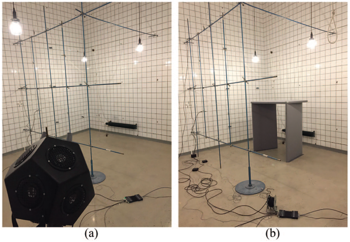
Measurement set-up and reverberant chamber: (a) empty reverberant room with the frame placed in position a and (b) reverberant chamber with absorbers inside and the frame placed in position a.

Type of excitation (performed in each of the previous cases)

Noise: the reverberant room was first excited with broadband noise band-passed from 10 to 100 Hz. The total length of the excitation was 105 s, including ramp-up time.

Pure tone: by comparing the simulation results with the measured frequency response obtained in the broadband excitation case, one of the eigenmodes of the room was chosen and further investigations were performed by exciting the room with that frequency.

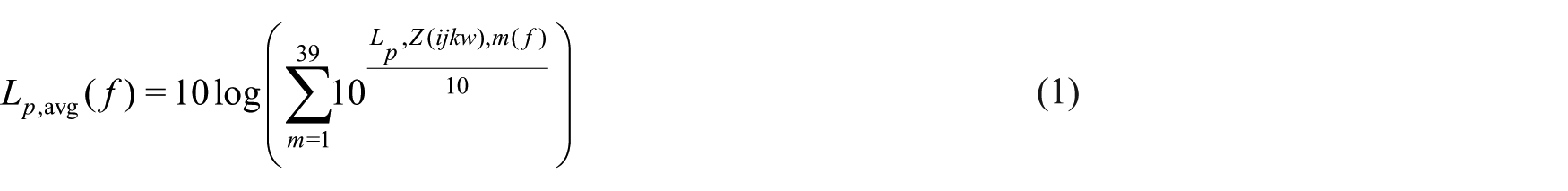
In total, four different scenarios were considered: (1) empty room with noise excitation, (2) empty room with tone excitation, (3) room with absorbers and broadband excitation and (4) room with absorbers and tone excitation. The individual signals for each microphone and each combination of case/excitation were obtained. The averaged frequency response (for each of the 39 measurement positions – 13 on each of the three planes $a$ , $b$ and $c$ ) was calculated with a frequency resolution of 0.03125 Hz (3200 lines) using 10 averages (i.e. 105 s of measurements in total for each measurement). The measurement files for each microphone position were saved and denoted following the nomenclature Z_i,j,k,w, where the subindex $i$ indicates whether the reverberant room is empty (0) or with the absorbers placed inside (1), $j$ denotes the type of excitation ( $b$ for broadband and $s$ for a pure tone), $k$ is the microphone position within each of the planes (k = 1, …, 13) and $w$ indicates the plane ( $a$ for the first one, $b$ for the second one and $c$ for the third one; cf. Figure 2). In this manner, for example, Z_0,s,10,b denotes an empty reverberant chamber, excited with a pure tone, at microphone position 10 and in the middle plane $b$ . In total, 156 files were acquired for postprocessing.

Figure 2.

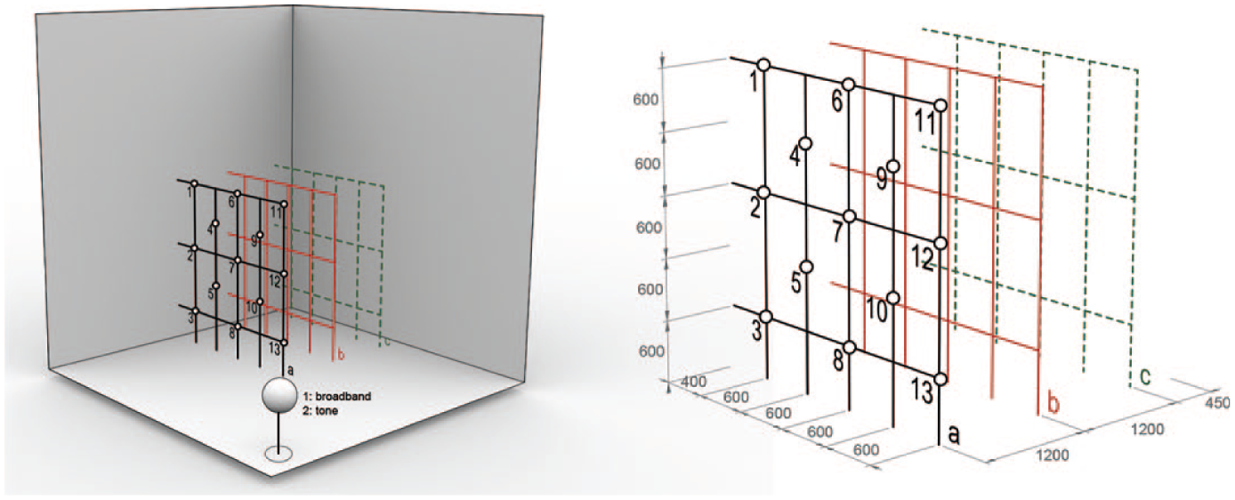
Sketch of the measurement set-up (left: whole room; right: frame dimensions). The numbers denote the different microphone positions within the frame for each plane (a in black colour, b in red and c in green). The sphere shown represents the dodecahedron loudspeaker emitting either broadband noise (b) or a tone excitation (s). For the sake of simplicity, no absorbers are placed in the figure.

Also, reverberation time measurements (performed according to ISO 3382-2:2008)¹³ were carried out using a sound level metre B&K 2270 in order to gain further knowledge about the reverberant chamber. It should be pointed out that at all times, the measurement equipment was controlled from a neighbouring room and no person was allowed to stay in the reverberant chamber during the data acquisition.

Simulations

An FE model of the reverberant chamber was set up in Comsol.²⁵ The air was meshed with acoustic tetrahedral elements, employing quadratic interpolation. The air properties were assumed to be bulk modulus K = 122 kPa and ρ = 1.22 kg/m³. The mesh size was decided based on the wavelengths expected to occur at the highest frequency of interest, namely, 100 Hz. The boundary conditions were initially set as rigid reflective walls, although other alternatives were eventually tried, as discussed in the following. First, a modal analysis was carried out on both the empty room and the room with the screens, to be able to adjust the model so that the frequency response of the room matched that of the simulated results.

Modelling the loudspeaker for performing steady-state analyses is a complex task and there is unfortunately no one general solution to it. Loudspeakers by different manufacturers are very different; they have different directivities and also sound source distributions (i.e. different parts of the surface of a loudspeaker could radiate differently and also the loudspeaker does not radiate equally in all directions). Different approaches can be adopted:

A brute-force approach, where a normal velocity boundary condition is applied to a surface mimicking the speaker. One can even make the velocity frequency dependent by making the amplitude an equation if that information is available from the manufacturer.

Pressure boundary condition acting as a pressure source at the boundary. In the frequency domain, the latter practically means that a constant acoustic pressure p₀ is specified and maintained as the amplitude of a harmonic pressure source.

Modelling the loudspeaker as a monopole, which is a source that radiates sound equally well in all directions. The simplest example of a monopole source would be a sphere whose radius alternately expands and contracts sinusoidally. The monopole source creates a sound wave by alternately introducing and removing fluid into the surrounding area.

Since a boxed loudspeaker at low frequencies is believed to act as a monopole, the latter approach was adopted in the simulations, it is being present at the lower corner where the actual loudspeaker was placed at during the measurement campaign. Further refinements of the source can be done eventually in later stages of the project. A frequency sweep in steps of 1 Hz was then carried out from 10 to 100 Hz.

Results

Broadband excitation

Measurements

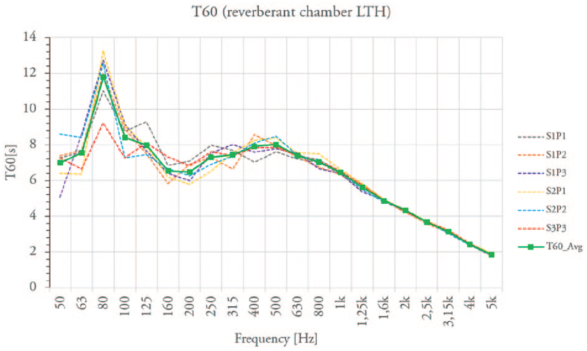
The results of the reverberation time measurements are shown in Figure 3. The average T₆₀ is 6.34 s. It is clearly depicted that below the Schroeder frequency $f_{S} ~ ~ 2000 (V / T_{60})^{(1 / 2)} = 360 Hz$ ; the field is of non-diffuse nature, which is of interest for the investigations reported here. Below that frequency, the recorded SPLs for different microphone positions vary much more than above it, pointing out a reverberant behaviour of the room as well as low modal overlap. This makes the spatial variations of the individual modes clear, and thus, the spread between the different measurement points will be evident.

Figure 3.

Reverberation time measurement results. Six different dashed lines are depicted, representing the results corresponding to three source positions, for which two microphone positions were considered (S_iP_j). Likewise, a frequency-averaged reverberation time is plotted as a solid green line.

The frequency-dependent averaged SPLs recorded in the measurements described in section ‘Measurements’, $L_{p, avg}$ , over all the microphone positions $m$ (39 for each case – empty/with absorber), was calculated according to the following

L_{p, avg} (f) = 10 \log (\sum_{m = 1}^{39} 10^{\frac{L_{p}, Z (i j k w), m (f)}{10}})

(1)

The results, plotted in Figure 4 (both for the empty room and for the room with absorbers), show that although there are certain peaks which are slightly displaced and/or damped (cf. Figure 4(b)), the overall (10–100 Hz) average difference between both cases is very low (2.6%). This is not surprising, as the screens have very low absorption at low frequencies. However, this points out that, even if different scenarios in rooms in dwellings (e.g. different type and/or distribution of furniture) may occur, measurement procedures based on statistical methods may lead to similar results, especially if SNDs are used. As a matter of fact, the equivalent SPL in both of the cases studied here (i.e. room empty and with absorbers included) are pretty similar (L_p,_eq,empty= 94 dB and L_p,eq,_absorbers = 93.5 dB). Half a dB is barely noticeable for the human hearing; however, nuisances from inhabitants can be reported by the fact that particular objects modify, at certain positions, the sound field in a room, and thus, much larger differences can occur than those predicted/described by averages or SNDs as it will be seen after. The latter can be very important and useful when designing rooms depending on their usage, as in that case, SPL averages may not be as important as the actual value for a certain position. Please note that the standard deviation of the SPLs is very small and thus omitted in the figures for the sake of clarity.

Figure 4.

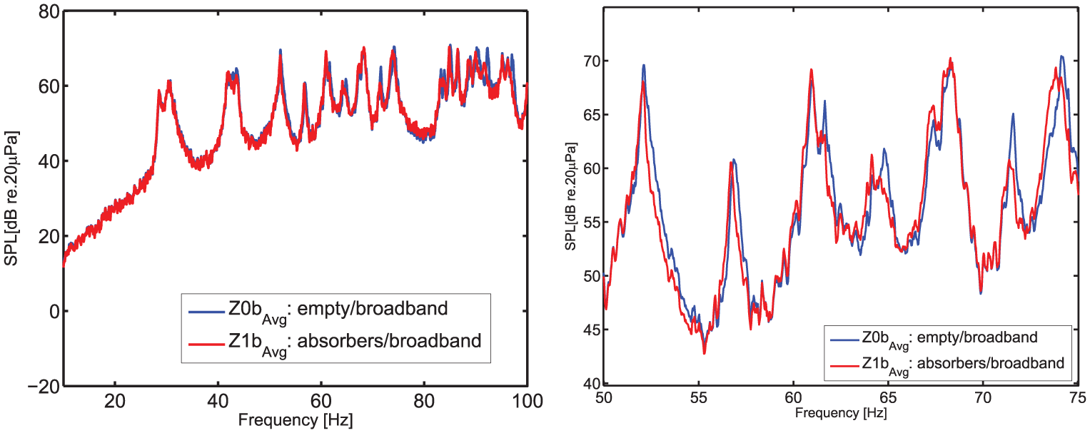
Averaged SPL over all microphone positions for both the empty room (blue) and the room with absorbers (red) for broadband excitation. The frequency average SPL is, in both cases, $L_{p, eq, empty} = 94 dB$ and $L_{p, eq, absorbers} = 93.5 dB$ : (a) frequency span 10–100 Hz and (b) zoomed in detail.

In Figure 5, some plots comparing the response recorded by microphones at the exact same position in both the empty room and with the screen absorbers are shown. Although at some positions the variations in SPL are not that large (cf. Figure 5(d)), approximately 45% of the measurement points showed a marked influence due to the changes in test set-up (i.e. introduction of absorbers) in certain frequency ranges. Furthermore, as depicted in Figure 5(a)–(c), not just a change in the room’s frequency response occurs, but also at certain eigenfrequencies differences up to 25 dB are found due to the simple presence of objects in the room (approximately 3 out of the 39 measurement positions showed differences exceeding 20 dB between both cases). Note that even though the absorption of the screens is very low within the frequency range analysed, the room’s response varies markedly. This highlights a potential need of accounting for other effects such as scattering or reflection when performing room designs in the low-frequency range, as modal behaviour may be of crucial importance.

Figure 5.

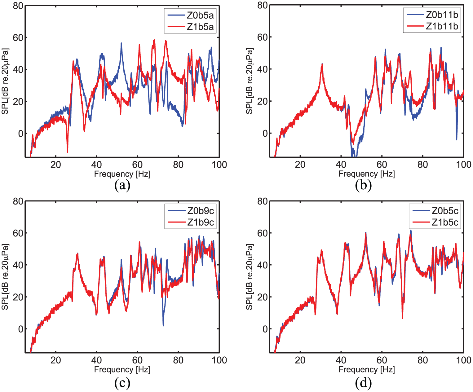
Comparison of the SPL recorded by microphones placed at the exact same positions in the empty room (blue) and room with absorbers (red) cases. The cases shown as an example involve different heights as well as planes within the room: (a) Z_0b5a versus Z_1b5a, (b) Z_0b11b versus Z_1b11b, (c) Z_0b9c versus Z_1b9c and (d) Z_0b5c versus Z_1b5c.

Simulations

An FE model of the room predicting the frequency response of the room was established (see details in section ‘Simulations’). Initially, hard reflecting walls were considered (its eigenfrequencies shown in Figure 6).

Figure 6.

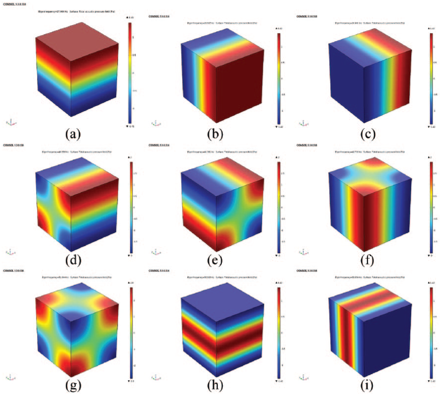
First 9 eigenmodes of the reverberant chamber under study, considering rigid walls. The colour legend shows normalised pressures, where blue and red correspond to high-/low-pressure values and green to zero-pressure values: (a) Mode 1: 27.96 Hz, (b) Mode 2: 29.97 Hz, (c) Mode 3: 30.46 Hz, (d) Mode 4: 40.95 Hz, (e) Mode 5: 41.35 Hz, (f) Mode 6: 42.70 Hz, (g) Mode 7: 51.04 Hz, (h) Mode 8: 51.93 Hz and (i) Mode 9: 59.85 Hz.

However, it was quickly noted that even though the room under study is a controlled case, boundary conditions as well as air properties can make it challenging when setting up a numerical predictive tool. Thus, a parametric study varying the impedance of the surrounding walls (a rigid, a calcareous and a tiled wall were considered – data from)²⁶ as well as different air properties (in terms of density and bulk modulus – considering an increase and a decrease of a factor of 2, respectively) was performed, the results being depicted in Figure 7(a). These parameters clearly influence the acoustic properties of the room, even for the simple case considered. After some adjustment of the wall impedances and air properties, an acceptable prediction of the eigenfrequencies of the room was achieved for the case using tiled walls (see Figure 7(b)). There are still small discrepancies found between measured and simulated eigenfrequencies, which can be, for example, due to the fact that small details (e.g. door, volume of the loudspeaker used for the measurements, lamps of the reverberant chamber) were not included in this preliminary model.

Figure 7.

Parametric studies. Comparison between simulated and measured results: (a) parametric studies performed in the anechoic chamber varying the impedance of the walls (rigid, calcareous, tiles) as well as air properties (density and bulk modulus). (b) Comparison of the measured averaged frequency response of the room (empty/broadband excitation) with the eigenfrequency simulated values (vertical black lines), up to 70 Hz, considering tiled walls.

The latter differences become markedly large if one, instead of looking at the eigenfrequencies alone, delves into the room’s frequency response (see Figure 8). There, one can see that although the correspondence is generally good, discrepancies between measured and simulated results (in both the empty and the room with absorbents case) are present. More specifically, an offset in the absolute values of the simulated results with respect to the measured ones, due, among other things, to the way the excitation (i.e. loudspeaker) was modelled (e.g. the sensitivity not taken into account) was observed. In Figure 8, and for the sake of making the comparison easier, an offset of −20 dB was applied to all the measured values. Further work is called for in the development of those numerical models in order for them to accurately predict the phenomena that is captured in the measurements. For example, the impedance boundary condition as well as the excitation source used should be refined.

Figure 8.

Comparison between simulated and measured results for broadband excitation. Note that an offset applied to all measured values in order to simplify the comparison: (a) empty room and (b) room with screens.

Closer analyses of the numerical analyses were performed by looking at some particular modes extracted from the frequency sweep. The room responses at 55, 65 and 89 Hz are shown in Figure 9. Although it is hard to assure whether or not the simulations show the same phenomena as captured by the measurements, it could be that the interaction between structural and acoustic modes modifies the symmetry of the modes (and thus the acoustic field inside the room) with respect to the empty case. This could explain what was shown in the measurements (see Figure 5), where microphones at the exact same position yielded very different SPL values (up to 25 dB) due to the presence of the screens. However, this has to be further investigated in the future by, for example, measuring the vibration levels of the screens, since in the modal analysis performed the loudspeaker was not modelled, nor the magnitude of the vibrations and thus the variations observed may also be a consequence of other things that dominate, and not just the acoustic–structure interaction.

Figure 9.

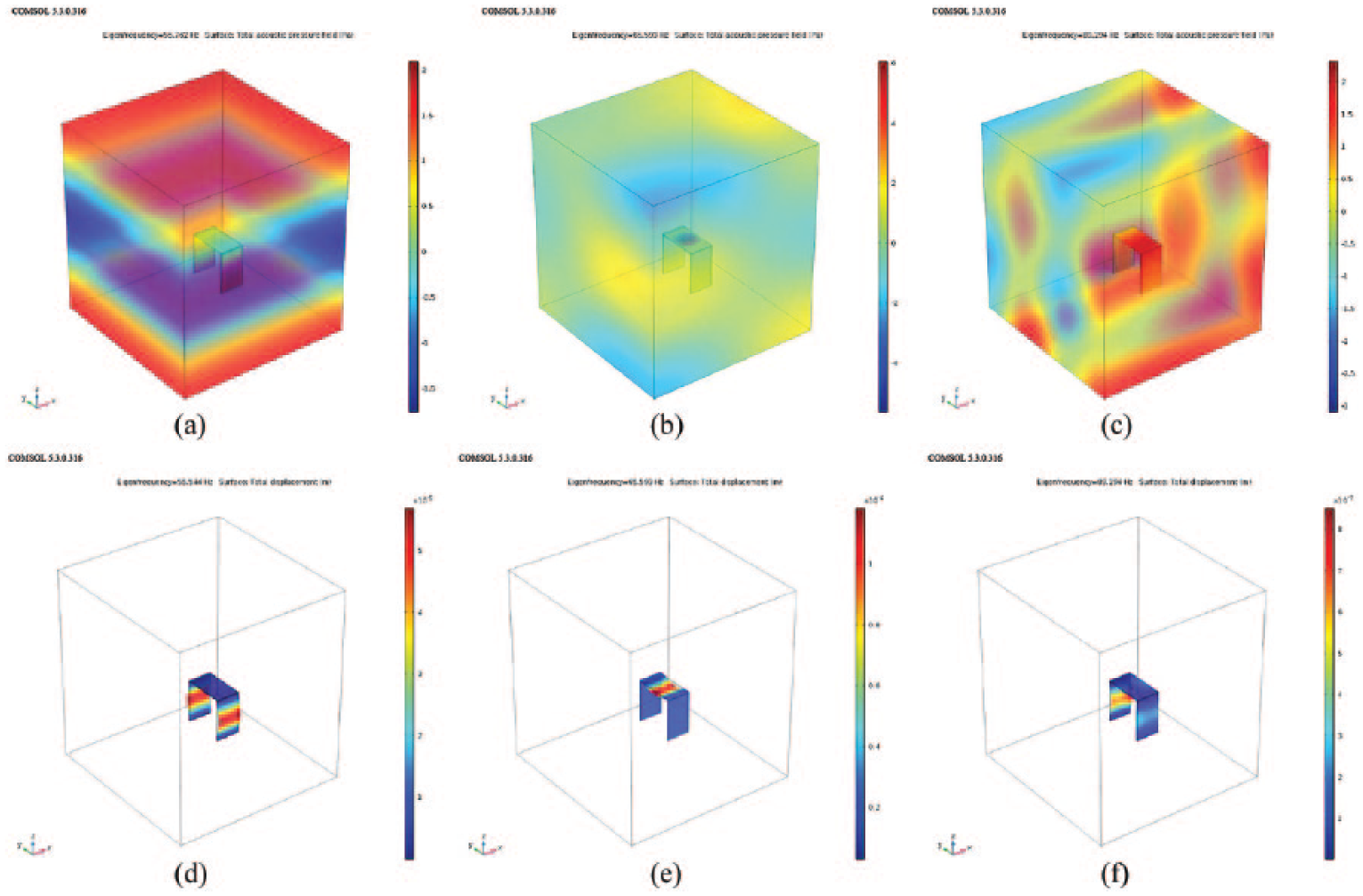
The colour legend of the room’s response (top figures) shows normalised pressures, where blue and red correspond to high-/low-pressure values and green to zero-pressure values. The screens’ response (bottom figures) depicts the mode shapes in terms of displacement, where blue means low-displacement values and red high deformations: (a) room’s response at ≈55 Hz, (b) room’s response at ≈65 Hz, (c) room’s response at ≈89 Hz, (d) screen’s response at ≈55 Hz, (e) screen’s response at ≈65 Hz and (f) screen’s response at ≈89 Hz.

Tone excitation

Based on the simulated results shown in Figure 7(b), one eigenmode was chosen for further investigations. The selected mode had a frequency of 61 Hz (see Figure 10(a) and the eigenmode analysis results depicted in Figure 6). The reason behind the choice was that (1) it should not be a too complex mode in the sense that differences in SPL over the room could be clearly detected and (2) that no other mode was too close in frequency so that they would not overlap in the measurements. The latter is important, as the fact that the room has fairly similar dimensions in all three directions makes the modes sometimes overlap (even in the few mode region) and hard to distinguish, especially in the measurement results.

Figure 10.

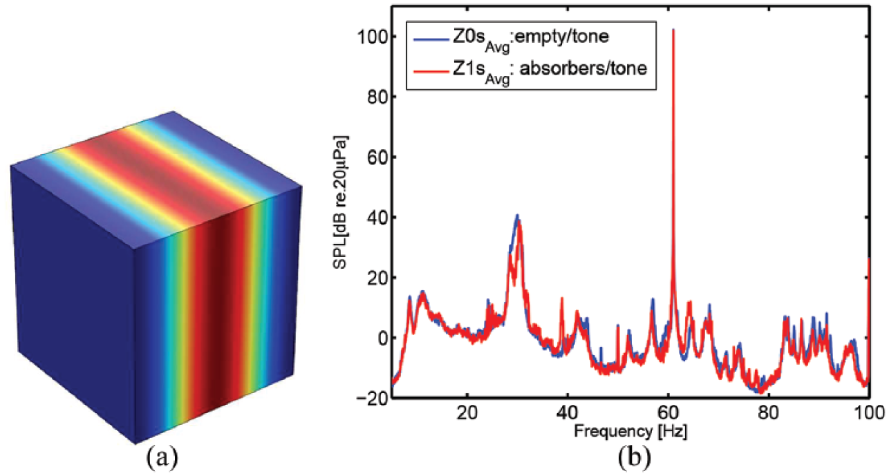
Tone measurement results: (a) room mode number 10 at 61 Hz and (b) averaged SPL over all microphone positions for both the empty (blue) room and the room with absorbers (red) for excitation at 61 Hz.

The fact that the eigenmode at 61 Hz was the same in the measured and simulated cases was proved by double checking the SPL measured by the microphones of the same plane ( $a$ , $b$ and $c$ ) at 61 Hz, since, according to Figure 10(a), they should all lie within a plane with approximately the same SPL distribution at that particular mode.

The room was then excited with a harmonic excitation coinciding with the chosen eigenfrequency, the results being shown in Figure 10(b). The overall (10–100 Hz) average difference between the empty and the ‘furnished’ room is higher than in the case of the broadband excitation (11% vs 2.6%). Nevertheless, the equivalent SPL in both of the cases is almost identical ( $L_{p, eq, empty} = 103.6 dB$ and $L_{p, eq, absorbers} = 103.9 dB$ ), due to, as pointed out before, the low absorption of the screens at this frequency.

Concluding remarks

In the investigations reported here, preliminary studies aiming at studying variations of the sound field that three moderately absorbing boards (emulating sparse furniture) can produce in a room were performed. Furthermore, the potential of numerical models as prediction tools for such problems was also pointed out.

The low-frequency properties of a room (where statistical methods in the standards cannot be applied directly) are often hard to estimate due to strong modal behaviour. It was shown that the SNDs do not reflect the variations in the field studied here, since the presence of particular objects in the room modified the sound field at certain positions in the room, yielding differences (comparing empty/room with furniture) of up to 25 dB. The latter difference was not captured by the SNDs. This should be further investigated in order to relate it with the acoustic comfort as perceived by the inhabitants and ultimately enable improved measurement methods.

The numerical models established in this preliminary investigation showed correct tendencies; however, further refinements and calibrations of the model (in terms of modelling the source as well as objects present, boundary conditions, etc.) are needed so that the absolute values can be accurately predicted. The results presented pave the way to future investigations as they showed the potential of such tools in order to address acoustic issues during the design phase of buildings. Such issues often call for costly and time-consuming measures such as construction of mock-ups and/or in situ measurements, and accurate numerical prediction tools could therefore reduce or eliminate these costs.

Footnotes

Declaration of conflicting interests

The author(s) declared no potential conflicts of interest with respect to the research, authorship and/or publication of this article.

Funding

The author(s) received no financial support for the research, authorship, and/or publication of this article.

ORCID iD

Juan Negreira

References

Negreira

Vibroacoustic behaviour of wooden buildings – prediction and perception. PhD Thesis, Division of Engineering Acoustics, Department of Construction Sciences, Lund University, Lund, 2016.

SS 25267:2004. Acoustics – sound classification of spaces in buildings – dwellings (in Swedish).

SS 25268:2004. Acoustics – sound classification of spaces in buildings – other premises.

Larsson

Simmons

. Vägledning för mätning av ljudnivåi rum med stöd av SS-EN ISO 10052/16032. SP rapport 2015-02 (in Swedish), https://www.sp.se/sv/units/risebuilt/hallbarsamhallsbyggnad/Omhallbarsamhallsbyggnad/Sektioner/eta/Documents/SP%20Rapport%202015_02.pdf

Simmons

Uncertainties of room average sound pressure levels measured in the field according to the draft standard ISO 16283-1. Akulite Report 3, SP Report 2012:28, https://www.traguiden.se/globalassets/forskning/akustik/akulite/akulite-rapport-3.pdf

Simmons

Measurement of sound pressure levels at low frequencies in rooms. Technical report 385, December 1997. Oslo: Nordic Innovation Centre.

Simmons

Larsson

. Measurement of time variant sound pressure levels at low frequencies in buildings – verification of sound class using EN ISO 10052 and 16032. In: Proceedings of euronoise 2015, Maastricht, 1–3 June 2015.

SS-EN ISO 16032: 2010. Acoustics – field measurements of airborne and impact sound insulation and of service equipment sound – survey method.

SS-EN ISO 16032: 2014. Acoustics – measurement of sound pressure level from service equipment in buildings – engineering method.

10.

Ljunggren

Öqvist

Simmons

Uncertainty of in situ low frequency reverberation time measurements from 20 Hz – an empirical study. Noise Control Eng J 2016; 64(6): 706–715.

11.

Hopkins

Turner

Field measurement of airborne sound insulation between rooms with non-diffuse sound fields at low frequencies. Appl Acoust 2005; 66: 1339–1382.

12.

Hopkins

Sound insulation. Amsterdam; Boston, MA: Elsevier, 2007.

13.

ISO 3382-1:2009. Acoustics – measurement of room acoustic parameters – part 1: performance spaces.

14.

Rindel

JH.

Sound insulation in buildings, Baton Rouge, LA: CRC Press, 2018.

15.

Jacobsen

A note on acoustic decay measurements. J Sound Vib 1987; 115(1): 163–170.

16.

Öqvist

Measurement and perception of sound insulation from 20 Hz between dwellings. PhD Thesis, Division of Operation, Maintenance and Acoustics Department of Civil, Environmental and Natural Resources Engineering, Luleå University of Technology, Luleå, 2017.

17.

ISO 717-1:2013. Acoustics – rating of sound insulation in buildings and of building elements – part 1: airborne sound insulation.

18.

ISO 717-2:2013. Acoustics – rating of sound insulation in buildings and of building elements – part 2: impact sound insulation.

19.

ISO 16283-1:2014. Acoustics – field measurement of sound insulation in buildings and of building elements – part 1: airborne sound insulation.

20.

ISO 16283-2:2014. Acoustics – field measurement of sound insulation in buildings and of building elements – part 2: impact sound insulation.

21.

ISO 10140-2:2010. Acoustics – laboratory measurement of sound insulation of building elements – part 2: measurement of airborne sound insulation.

22.

ISO 10140-3:2010. Acoustics – laboratory measurement of sound insulation of building elements – part 3: measurement of impact sound insulation.

23.

Prato

Schiavi

Sound insulation of building elements at low frequency: a modal approach. Energy Proced 2015; 78: 128–133.

24.

Brüel and Kjær. PULSE reflex 20.0. Copenhagen: Brüel & Kjœr Sound & Vibration Measurement A/S.

25.

COMSOL Multiphysics. COMSOL multiphysics v. 5.3. Stockholm: COMSOL Multiphysics.

26.

Piechowicz

Czajka

Determination of acoustic impedance of walls based on acoustic field parameter values measured in the room. Acta Phys Pol A 2013; 123(6): 1068–1071.