Home affordability,female marriage rates and vote choice in the 2000 US presidential election

The geographic sort

The issue of the political sorting of the American electorate is not new in political science. It provides a cogent explanation for increasing levels of political polarization. Whereas the political landscape at the national level in the 1950s and 1960s was characterized by ideologically heterogeneous political parties – including a large number of liberal ‘Rockefeller’ Republicans and conservative Southern Democrats – American politics at the Congressional level today is characterized almost exclusively by conservative Republicans and liberal Democrats (McCarty et al., 2006; Theriault, 2008). The comparative ideological homogeneity of the two major parties has proved conducive to ideological extremism within the two parties and the incentives to compromise have waned (Brownstein, 2007). However, this increasing ideological extremism in Congress has not necessarily been reflected among the electorate as a whole; some evidence suggests that individual voters are not any more or less ideological than they were in the past (Fiorina, 2005). An explanation for this seeming incongruity can be found in the partisan sorting of the electorate along ideological lines. Matthew Levendusky (2009) provided strong evidence that political polarization has been driven by individual voters joining the party that accurately reflects their ideological disposition, that is, most political liberals are now Democrats and most political conservatives are now Republicans.

A major political sort along geographic lines has also recently received substantial attention. Although the entire nation remains politically diverse, many small political units are not. Increasingly, cities, counties and even entire states have become quite politically homogeneous. Gimpel and Schuknecht described the clustering of like-minded voters along geographic lines in Patchwork Nation (2006). More recently, Gimpel and Dante Chinni launched a website (2008) of the same name exploring characteristics of different kinds of political communities. Based on factor analysis, these scholars divided the nation into 12 different kinds of communities – such as ‘boom towns', ‘monied ‘burbs' and ‘Mormom outposts' – that exhibit certain cultural, political, economic and demographic characteristics.

In their book, The Big Sort (2008), Bill Bishop and Robert Cushing further explored the clustering of Americans along political lines. Bishop and Cushing noted that an increasing number of counties in the United States have become dominated by a single political party. As a result, politics, at least at the county level, is increasingly less competitive and dominated by ideological extremists. To demonstrate their point, Bishop and Cushing pointed to the total number of landslide counties in the United States (defined as counties in which one party in a presidential election won by 20 percentage points or more). In the 1976 presidential election, only a little more than 26 percent of the population lived in landslide counties; by 2000, that number was 45.3 percent. ¹

Bishop and Cushing argued that much of this can be explained by the increasing levels of choice voters have in regard to where they live. In comparison to other periods in American history, citizens have an unprecedented ability to move to where they will be happiest, which frequently means that individuals choose to live among like-minded people. Other scholars have also considered how the clustering of like-minded individuals influences American politics. Richard Florida (2002), for example, described what he called America’s ‘Creative Class', which tends to vote Democratic and live in certain large cities.

There are potential normative implications of the geographic sort. As regions become increasingly homogeneous, the two-party system may fail to work effectively. In such regions of the country, incumbents from one party are assuredly less likely to be defeated by a challenger from the opposition party, and both parties have increased incentives to pander to ideological extremes to avoid successful primary challenges.

Although the phenomenon of geographic sorting and the increasing number of landslide counties has been well described, there remains relatively little work explaining why some previously competitive counties become Republican strongholds and others Democratic. Some of this trend can undoubtedly be traced back to path-dependent processes that began decades or even centuries ago. Those strong Republican counties that Gimpel and Chinni described as ‘Mormon outposts', for example, are probably best explained by the migration patterns of early Mormon settlers. In this article, however, I am interested in finding contemporary economic or other variables driving today’s geographic sorting along partisan lines. Drawing heavily on previous scholarship on home-ownership and the ‘marriage gap’ (Gershkoff, 2009; Kingston and Finkel, 1987; Plutzer and McBurnett, 1991), I hypothesize that one characteristic that distinguishes Republican counties from Democratic counties is the relative affordability of single-family homes.

Specifically, I test the hypothesis that relatively affordable housing was associated with more support for George W. Bush in the 2000 election at the county level. Although the relationship between home-ownership and partisanship has been examined previously (Blum and Kingston, 1984; Verberg, 2000), most such studies consider home-ownership primarily as it relates to economic well-being or incorporation into the community. I offer an alternative hypothesis. I hypothesize that home affordability at the aggregate level is relevant to political outcomes even when controlling for economic variables such as median income and poverty rates. I argue that home affordability is relevant to politics largely because of its relationship with marriage rates within geographic units, which subsequently influences political outcomes because of the partisan marriage gap.

Put less abstractly, I suggest that married couples are more likely than single individuals to want to own their own home. However, there are some areas where home-ownership is prohibitively expensive, especially for younger Americans. If young couples living in those high-housing-cost communities want to own their own house, they have no choice but to move. Thus, I anticipate that the marriage rates within a county can be at least partially explained by the average housing costs within that county. Because, as the political science literature suggests, married voters are more likely to vote Republican than non-married voters, this trend leads some counties to become increasingly Republican, and others increasingly Democratic.

The marriage gap

The idea of a marriage gap in American politics has spurred much debate among political scientists. Herbert Weisberg (1987) noted that married voters are about 10–15 percent more Republican than non-married voters. Looking at 1982 Congressional elections, Martin Plissner (1983) found that non-married voters favoured Democrats by 26 percentage points. Edlund and Pande (2002) argued that the increasing liberalism among female voters was directly related to declining marriage rates.

It is easy to imagine plausible causes of a partisan marriage gap. Marriage is traditionally associated with raising children, which should decrease an individual’s tolerance of social disorder and hence lead to cultural and/or political conservatism (Plissner, 1983). It is furthermore intuitive that the Republican Party’s message of ‘family values' will be more persuasive to those voters who are currently married and raising children. In a study that focused exclusively on women, Kathleen Gerson (1987) found evidence that the marriage gap among women resulted from different orders of preferences, with married women tending to be more concerned with domestic commitments, and non-married women being more concerned with issues such as career opportunities and gender equality.

The existence, strength, or causes of a marriage gap in vote choice is not the primary concern of this article. However, a cursory look at the 2000 presidential election returns suggests that the average marriage age was a strong predictor of George W. Bush’s share of the vote. Figure 1 shows the relationship between the average female age at first marriage (as reported by the US Census) and the percentage of the vote earned by Bush in 2000 at the state level, and demonstrates that, as the average marriage age increased, Bush’s share of the vote dropped dramatically. Given the strength of this relationship, it can be plausibly argued that even a small change in the average marriage age and in total marriage rates within a geographic unit will have a meaningful influence on political outcomes within that unit.

OPEN IN VIEWER

Figure 1.

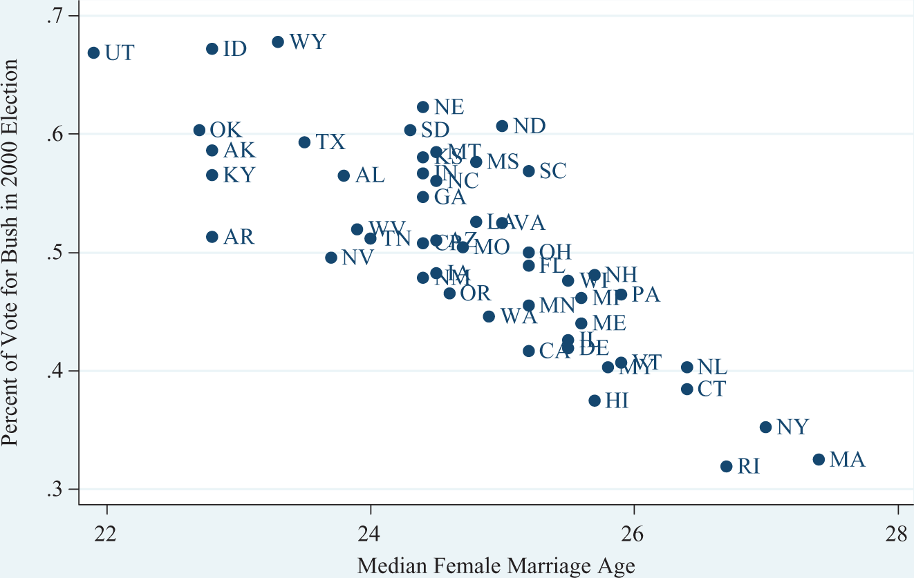
Marriage age and support for Bush by state.

Housing costs and marriage rates

As stated previously, the marriage gap is relevant to this study because the degree to which a county or city is considered a good place for married couples to stay or settle may explain some aspects of America’s partisan geographical sorting. Assuming that most individuals prefer to live in their own home rather than a condominium or apartment after forming a family unit, one indicator of a city or region’s attractiveness for married couples is the cost of housing. For decades, the sociology literature has suggested that decisions regarding marriage and family formation are related to housing and other costs (Goodsell, 1937). John Hajnal (1965) argued that the rising average age of marriage in Western Europe resulted from the decreasing amount of available land for housing. Landale and Tolnay (1991), looking at the American South, also found that land availability affected the average marriage age. Felson and Solaun (1975) found evidence suggesting that renting an apartment, as opposed to owning a house, leads to lower fertility levels, which supports the hypothesis that family formation is positively affected by the ease of home-ownership.

The possible relationship between home affordability and aggregate voting trends has largely been ignored up until now by the political science literature, though the topic has been considered by the political journalist Steven Sailer (2008). Sailer hypothesized that ‘affordable family formation’ – which he argued was closely related to housing costs – was a key difference between majority-Republican states and majority-Democrat states. Sailer went on to conclude that the relative affordability of housing accounted for the differing typical political behaviour within various large cities. Sailer suggested that the relative costliness of owning a home in America’s large coastal cities, such as Los Angeles, led to later family formation, which partially explained the greater support for Democratic politicians in those cities and regions. In contrast, inland American cities like Dallas are able to expand outward all-but indefinitely, which keeps housing costs low and subsequently such cities more attractive to young families.

Because it draws from a wide variety of literature, and may at first seem counterintuitive, it may be useful to reiterate my hypothesis and proposed causal mechanism. I argue that affordable housing is associated with greater support for Republican candidates because, as the sociology literature suggests, marriage rates are associated with the relative affordability of single-family homes, and, as the political science literature demonstrates, ideology and vote choice are at least partially predicted by marital status, particularly for women. I should also make clear what I am not suggesting. I do not argue that living in a community with affordable housing causes people to get married at a younger age. Rather, my intuition is that, given the relative ease of geographic mobility in the United States today (Bishop and Cushing, 2009), young married couples tend to gravitate toward areas where they can own a home of their own. I am also not arguing that getting married causes young women to change their partisan affiliation – though for young people of either gender without strong, previously established partisan preferences, this may occur. Rather, I suspect it is more likely that the decision to get married at an early age is motivated by other variables strongly associated with vote choice – religiosity (Thornton et al., 1992) or income prospects (Bergstrom and Schoeni, 1996), for example. I argue, instead, that home values contribute to the geographic sorting of the population, but do not necessarily influence the overall distribution of votes between the major parties in the nation as a whole.

Aggregate-level evidence

My dependent variable for the models testing my hypothesis regarding home values and vote choice was the percentage of the vote earned by President George W. Bush at the county level in the 2000 presidential election. My key independent variable for the models of aggregate vote choice was housing affordability at the county level, which I measured with the median value of owner-occupied housing units. These data, like all the aggregate economic and demographic data used as control variables in the models presented here, were taken directly from the US Census.

Because so many variables that correlate with home values also correlate with aggregate voting patterns, it was important to include a wide variety of control variables to ensure I am not reporting a spurious relationship. Perhaps the most important control variable to include in this model was median income, because of its high correlation with home values (Pearson’s r = 0.65) and strong relationship with vote choice at the county level.

One could think of other explanations for the relationship between home values and vote choice. For example, one could posit that home values are correlated with aggregate vote choice as a result of the ‘rural brain drain’ (Carr and Kafelas, 2009). That is, perhaps many of my findings are a result of young, educated people rapidly leaving certain regions of the country, such as the rural areas of the Midwest and Great Plains, to pursue career opportunities in urban centres. As they leave, they leave behind counties that are increasingly older, and hence more Republican (Sokhey and Djupe, 2009), and characterized by low property values. I will not say that it is not possible that this explains at least part of the phenomenon I am exploring here. I believe, however, that I have included a sufficient number of variables to control for this possibility. By controlling for both median age and the percentage of a county’s population classified as rural, I can ensure that my findings are not merely a result of young people fleeing rural communities.

I also controlled for the percentage of African Americans and Hispanics within a county – a necessary control because of these demographic groups' relatively lower average socio-economic conditions and strong preference for Democratic over Republican candidates. A variable was also included for the percentage of the population within a county that had completed a four-year college degree, which is correlated with incomes, home prices and marriage age. I also included the percentage of the population below the poverty line, as specified by the Census Bureau. In case there are systematic cultural, economic or other differences between the various regions in the United States, I included regional control variables for the nine census regions, with New England as the base category.

Because it was of importance to my theory, I also created a model controlling for marriage rates among young women in order to see how the inclusion of this variable influenced the coefficients of other variables. Ideally, the best variable for this model would have been the median marriage age at the county level. Unfortunately, although the US Census reports this variable for states, it does not provide it for counties. However, measuring the rates of marriage within a specific age cohort can likely provide a strong indication of the median marriage age. ² To that end, I included as an independent variable the percentage of women between the ages of 25 and 30 who have ever been married, which includes those married at the time of the census, those widowed, those separated and those divorced. I looked at women exclusively because the literature suggests that the marriage gap is stronger among women. By creating this model I hoped to verify that the electoral marriage gap could be demonstrated statistically in the 2000 election at the county level.

To further test my hypothesis that home affordability influences partisanship at least in part because of its influence on marriage age, I created a model in which the percentage of women between the ages of 25 and 30 who have ever been married was the dependent variable. This allowed me to develop a greater understanding of exactly how home values influence average marriage rates within counties. Next, to see how changes in the housing market influence changes in aggregate voting behaviour, I created a model examining whether changes to the median cost of a single-family home influenced changes in voting patterns over time. Specifically, I modelled changes in the county-level vote totals from the presidential elections in 1980 to 2000 as a function of changes in housing costs between those years.

Finally, I supplemented the aggregate models with models using individual-level survey data. All individual-level data were provided by the 2000 National Annenberg Election Survey.

I excluded Alaska and Hawaii from this analysis, as well as those island counties with no contiguous neighbours, because of the difficulty in incorporating them into spatial-lag models. I also excluded counties that had missing data.

Visual evidence

Before creating any models predicting support for Bush at the county level, I visually examined how my variables of interest were distributed across the country. Figures 2 and 3 show how support for Bush and relative home affordability were distributed across the United States in 2000. In creating this figure, I needed to use a simple measure of home affordability. To create such a measure, I simply divided the median home value by the median income. A county with a value of 3 for this measure, for example, is a county in which the median owner-occupied home is valued as being worth three years of the median household income. This variable provides a rough estimate of how economically easy or difficult it is to own a home within a county. In Figure 2, lighter-shaded counties are associated with more support for Bush at the county level, whereas darker-shaded counties are associated with less support for Bush. In Figure 3, we can see how home affordability varies across the nation. In this figure, dark-shaded counties are associated with high-median income-median home value ratios, whereas light counties are associated with lower ratios.

OPEN IN VIEWER

Figure 2.

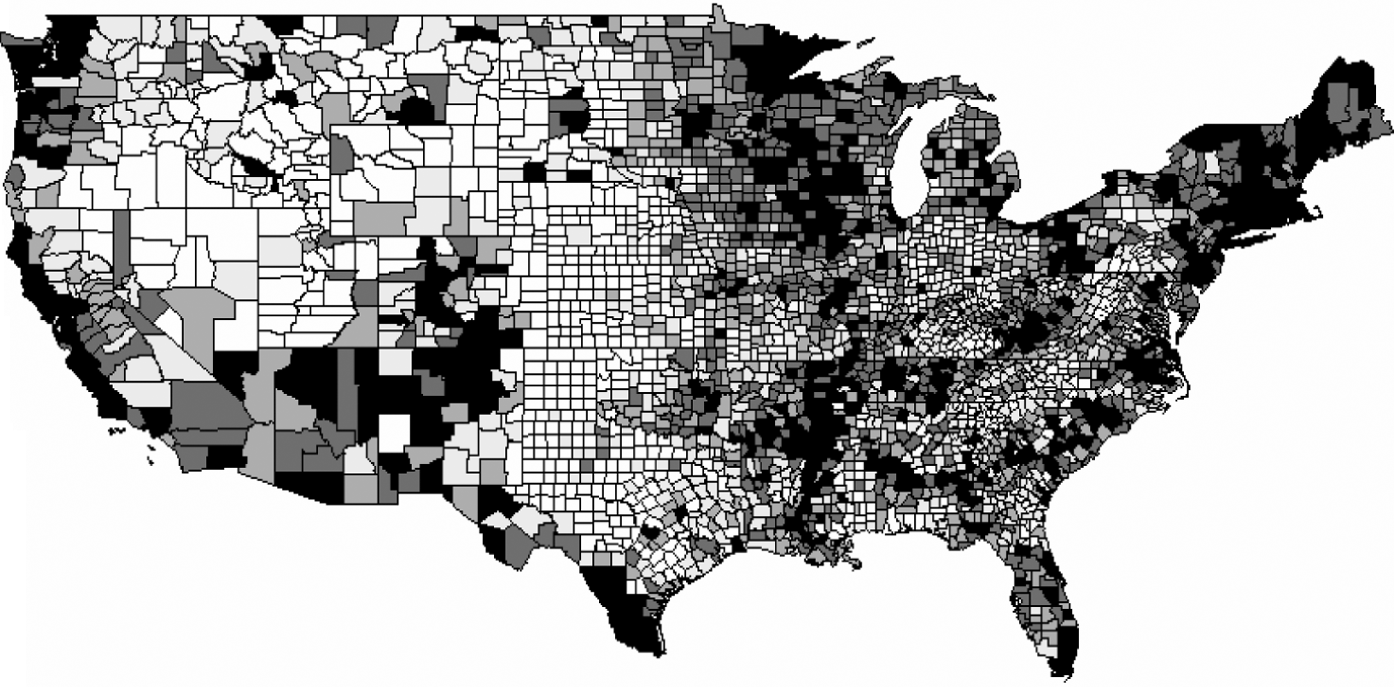
Support for Bush at the county level in 2000.

OPEN IN VIEWER

Figure 3.

Median income–median home value ratio in 2000.

From these figures we can see that the two measures correspond quite highly. In general, support for Bush was much lower in the regions where housing costs were high than in the relatively inexpensive regions. There are a few regions where voting behaviour clearly does not conform to my theory, however. In some cases, this can be explained by the racial/ethnic characteristics of those counties. Within the heavily Hispanic counties in southern Texas, and the heavily African American counties along the Mississippi river, for example, my measure of home affordability shows that houses were actually quite affordable. However, these counties went heavily for Gore. This is likely because black and Hispanic voters tend to vote more heavily for Democrats regardless of their economic conditions.

The more interesting incongruity with my theory is in the Mountain West. Based on my measure, it is clear that this region was not characterized by particularly affordable homes, yet was generally rather supportive of Bush. For example, some counties in Colorado had, on average, some of the least affordable homes in the country. Yet in 2000, Colorado was a solidly Republican state. However, in the years following 2000, Colorado rapidly changed politically, swinging from a heavily Republican state, to a swing state, to what now appears to be a strongly Democratic state – President Obama won 54 percent of the vote in Colorado in 2008. It may be the case that changes in home affordability take some time to influence partisan behaviour. Understanding what is going on here is made further complicated because of the massive amount of in-migration this region experienced in recent decades that has had a major influence on electoral outcomes (Robinson and Noriega, 2010).

The spatial-lag model

Figures 2 and 3 suggest a problem with using basic OLS models to test my hypotheses. The degree to which the values for these variables tend to cluster together in different regions suggests that spatial autocorrelation is potentially a serious concern. As with temporal autocorrelation, the presence of spatial autocorrelation violates the OLS assumption of independence among the observations. The Moran’s I for my dependent variable was a statistically significant 0.58. This statistic confirmed the presence of spatial autocorrelation, suggesting that the spatial relationship must be controlled for in order to draw valid inferences.

Models with spatially lagged dependent variables are commonly used to correct for spatial autocorrelation. The spatial-lag model can be written as follows:

y = β x + ρ W y + ε i

Where ρ is a spatial autoregressive coefficient and W is a connectivity matrix. The logic behind spatial-lag models is similar to that of time-series models with temporally lagged dependent variables. However, estimation of ρ in a spatial model is complicated because, unlike temporal autocorrelation, spatial autocorrelation is bi-directional and two-dimensional. Therefore, ρ in a spatial model can only be estimated accurately via maximum likelihood.

A decision had to be made regarding how to deal with the different population sizes of each county. Failing to control for population at all would have given disproportionate weight to the nation’s hundreds of sparsely populated counties. One option was to attach analytic weights to each observation, which would specify the importance of each observation based on its total population. Another option was to simply include each county’s total population as an independent variable. I chose the latter option for the models reported in this article. My primary interest was in the electoral outcomes at the county level, rather than the individual level, and weighing each county by population would have made drawing inferences about an individual county’s aggregate voting behaviour more difficult.

Home affordability and aggregate vote choice

The estimates for the spatial regression models using aggregate county data can be found in Table 1 . In these models, ρ is quite large and highly statistically significant, meaning that the value of the dependent variable for each of these counties could be largely inferred from the value of the dependent variable in neighbouring counties. Even when controlling for autocorrelation, however, the basic intuitions driving this article were confirmed. In Model I, we see that, on average and controlling for all other variables, a $10,000 increase in the median home value was associated with 0.3 fewer percentage points for Bush at the county level, and a 2 SD increase in the median home value at the county level was associated with 2.5 fewer percentage points for Bush. We see, further, that even though median home values and incomes are highly correlated, they have an opposite effect on aggregate vote choice – as median incomes increased, support for Bush also increased.

OPEN IN VIEWER

Table 1.

County-level spatial lag models 2000

	Model I % for Bush	2 Std. Dev. Δ	Model II % for Bush with Marriage Mediator	2 Std. Dev. Δ	Model III % of Females Married Age 25-30	2 Std. Dev. Δ	Model IV Change in Vote % for Republican 1980-2000†	2 Std. Dev. Δ
Median income (divided by $10,000)	2.9 (0.5)**	4.6	2.4 (0.5)**	3.8	2.8 (0.6)**	4.5	1.8 (0.4)**	1.7
Median home value (divided by $10,000)	–0.3 (0.1)**	–2.5	–2 (1.0)**	–1.9	–0.3 (0.1)**	–2.6	–0.5 (0.1)**	–2.3
% of females married age 25-30	−	−	0.2 (0.0)**	5.5	−	−		−
Median age	0.1 (0.1)	−	0.0 (0.0)	−	−	−	0.0 (0.1)	−
% with BA	–0.1 (0.0)**	–2.1	0.0 (0.0)	−	–0.6 (0.0)**	–9.1	–0.1 (0.0)*	–1.0
% Rural	0.1 (0.0)**	3.2	0.0 (0.0)**	2.5	0.1 (0.0)**	3.6	0.0 (0.0)	−
% Black	–0.1 (0.0)**	–3.6	0.0 (0.0)*	–1.2	–0.2 (0.0)**	–7.6	–0.2 (0.1)	–1.45
% Hispanic	0.0 (0.0)	−	0.0 (0.0)	−	0.0 (0.0)	−	0.0	−
% in poverty	–0.3 (0.1)**	–4.2	–0.3 (0.1)**	–3.2	–0.3 (0.1)**	–4.3	–0.5 (0.1)**	–6.3
Total county population (divided by 10,000)	0.0 (0.0)**	–1.3	0.0 (0.0)**	–1.2	0.0 (0.0)**	–0.8	–0.1 (0.0)**	–1.3
Pacific	4.3 (0.9)**	−	3.1 (0.8)**	−	5.1 (0.9)**	−	3.2 (0.7)**	−
Mountain	5.1 (0.8)**	−	3.4 (0.7)**	−	7.1 (0.8)**	−	3.4 (0.6)**	−
West North Central	1.2 (0.5)*	−	0.0 (0.5)	−	3.8 (0.6)**	−	0.1 (0.5)	−
East North Central	–0.8 (0.5)	−	–0.9 (0.5)*	−	1.5 (0.6)**	−	0.8 (0.5)	−
West South Central	6.1 (0.6)**	−	3.1 (0.6)**	−	10.1 (0.7)**	−	4.4 (0.7)**	−
East South Central	5.1 (0.7)**	−	2.6 (0.6)**	−	8.1 (0.6)**	−	2.8 (0.7)**	−
South Atlantic	5.2 (0.6)**	−	3.5 (0.6)**	−	6.3 (0.6)	−	2.2 (0.6)**	−
Mid Atlantic	1.8 (0.6)**	−	2.5 (0.5)**	−	–1.3 (0.6)**	−	0.3 (0.6)	−
Constant	3.6 (3.2)**	−	–13.1 (3.4)**	−	47.3 (4.0)**	−	6.1 (1.3)**	−
ρ	0.8 (0.0)**	−	0.8 (0.0)**	−	0.4 (0.0)**	−	0.8 (0.0)**	−
Observations	3103		3103		3103		3103
Robust LM test	1965.1		1868.6		229.9		1150.7
P-value	0.0		0.0		0.0		0.0
Variance ratio	0.7		0.7		0.7		0.5

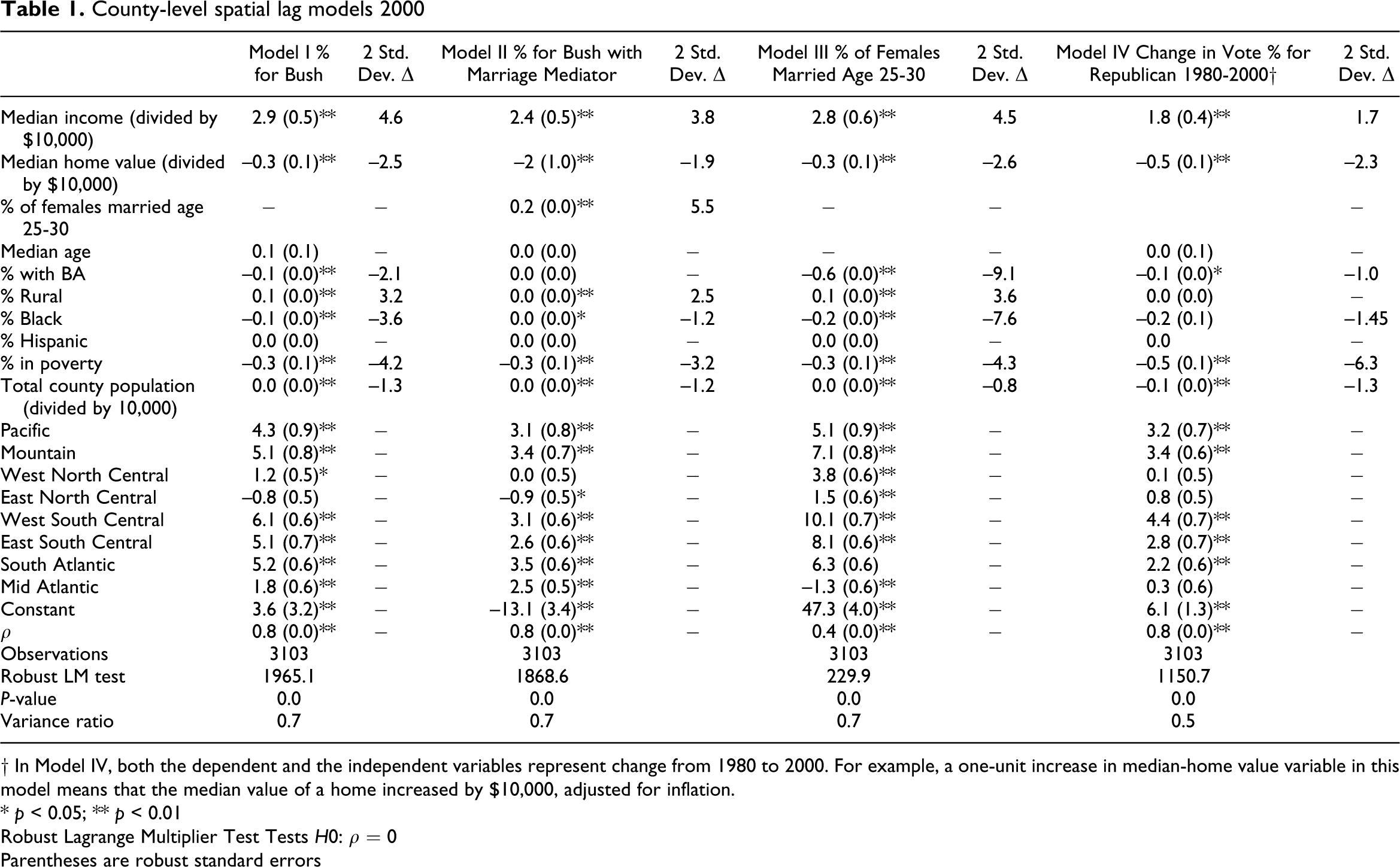
† In Model IV, both the dependent and the independent variables represent change from 1980 to 2000. For example, a one-unit increase in median-home value variable in this model means that the median value of a home increased by $10,000, adjusted for inflation.

* p < 0.05; ** p < 0.01

Robust Lagrange Multiplier Test Tests H0: ρ = 0

Parentheses are robust standard errors

Because I hypothesized that part of the explanation for home values' influence on aggregate vote choice was due to the relationship between vote home values and marriage rates, I created a separate model that included marriage rates among women between the ages of 25 and 30 as an independent variable. We see in Model II that the inclusion of this variable decreases the size of the coefficient for median home values. It does not, however, wipe out its effects entirely. In fact, the relatively small effect this mediator variable had on the coefficient for home values suggests that home values also influence vote choice for reasons unrelated to marriage rates. That is, perhaps home values are also associated with other economic variables that influence vote choice. What is most remarkable about Model II is the strength of the marriage rate variable. This variable had a greater influence on vote choice at the county level than any other variable, including income. The strength of this variable may seem strange given that the total percentage of the population that falls in this category is relatively small. I should therefore reiterate that this is a somewhat imperfect variable for what I want to measure. My main interest is not in just this age cohort specifically, but in the county’s median age at first marriage, which this measure is only able to capture indirectly. It is interesting to note that, when this variable was included, education rates ceased to have any statistically significant effect on aggregate support for Bush. This finding provides strong new evidence that the partisan marriage gap is a meaningful determinant of election outcomes. These aggregate data further suggest that the education gap in politics is largely a function of the degree to which higher education tends to depress marriage rates for young people.

Home affordability and marriage rates

Given that I argued that lower home values increased support for Bush specifically because of the relationship between home values and marriage rates within a county, I also modelled that relationship. In these models, the percentage of women between the ages of 25 and 30 who were married in 2000 was the dependent variable and the median cost of an owner-occupied home once again was the key independent variable. In Model III we see that a $10,000 increase in the median home value was associated, on average, with a 0.3 decrease in the marriage rate among women of this age. A 2 SD change in this variable was associated with 2.6 percent fewer women between the ages of 25 and 30 who have ever been married. All of this provides further evidence for my hypothesis that home values influence aggregate vote choice at the county level at least partially because of the relationship between home values and marriage rates.

Although the problem of ecological inference means I must use caution before drawing strong conclusions, Model III provides other interesting findings, as well. As was the case with support for Bush, the direction of the coefficients for median income and median home value were in the reverse direction. We also see, as Model II suggested, that education rates had a substantial influence on marriage rates among women of this age cohort. A 2 SD increase in the percentage of the population with a bachelor’s degree (BA), a variable that was also associated with income, was associated with a more than 9 percent drop in the marriage rates of women in this age cohort. Poverty, however, also depressed marriage rates.

Changes in voting patterns and changes in housing costs

These findings provide strong evidence that home values influenced vote choice at the county level in the 2000 election. It tells us nothing, however, as to whether changes in a county’s home values subsequently lead to changes in aggregate vote choice. To test whether such a relationship exists, I created a model for the change in the percentage of the vote received for the Republican candidate from the 1980 election to the 2000 election; that is, the different percentage of the vote received by George W. Bush at the county level in comparison to the percentage of the vote received by Ronald Reagan. ³

From Model IV, we see that changes in support for the Republican presidential candidate at the county level were at least partially a function of other county-level changes in demographic and economic characteristics. Given that Ronald Reagan won the 1980 election by a strong margin and George W. Bush won the 2000 election by a tiny margin (and actually lost the popular vote), it is not surprising that most counties gave less support to the Republican candidate in the latter election – on average, George W. Bush in 2000 received 1.29 fewer percentage points per county than Ronald Reagan in 1980. However, in the counties where housing prices rose at a higher rate, the Republican candidate lost more votes even when controlling for other changes. In counties that experienced a 2 SD increase in home values, again controlling for all other variables and spatial autocorrelation, Bush received 2.3 fewer percentage points than Reagan in 1980. In fact, when looking at change over time, we can see that changes in home values had a stronger influence on changes in the aggregate vote change at the county levels than changes in the median income – though this was likely partly a function of my decision to also control for changes in poverty rates, which are highly correlated with changes in income. More sophisticated time-series methods should be employed in examining this question in the future, but these results seem to indicate that political change over time can at least be partially predicted by changes in housing markets.

Individual-level evidence

To assuage any concerns that I am engaging in the ecological fallacy (Robinson, 1950), I must emphasize that my main units of interest are the counties themselves, rather than individuals. However, I was able to supplement my aggregate-level findings with individual-level survey data from the 2000 National Annenberg Election Survey. This survey is ideal for these kinds of questions because of its large n as well as the inclusion of county-level Federal Information Processing Standards (FIPS) codes. This allowed me to include county-level variables in a multi-level regression model (Steenbergen and Jones, 2002).

The dependent variable for Model V was vote choice in the 2000 election. As was the case in the aggregate models, my key contextual independent variable was the county’s median home value. Like the earlier models, I also controlled for the median income, as this has also been demonstrated to influence individual vote choice (Gelman et al., 2007). I also included three dummy variables for whether the individual lived in an urban, suburban or rural area – with rural as the base category.

Individual-level variables included conservatism (a 5-point variable ranging from 0, very liberal, to 5, very conservative), marital status (a dummy variable coded 1 if married), female, an interaction between marriage and female to determine, at the individual level, if the marriage gap really is stronger for women than men, household income, age, whether the respondent earned a BA, race (coded 0 for non-black, 1 for black), and ethnicity (coded 0 for non-Hispanic, 1 for Hispanic). As was the case with aggregate data, I also created a model in which marital status was the dependent variable (Model VI). In case there were systematic differences in different regions of the country, I also include a level for census region. Thus, given the dichotomous nature of the dependent variable, I specified a three-level hierarchical logit model, with individuals being the first level, counties the second and regions the third.

Results for the multi-level models are given in Table II. These individual-level results are consistent with the aggregate-level findings reported in Table 1. Of particular interest is the finding, in Model V, that county-level median home values had a statistically significant influence on the probability that an individual would vote for Bush in 2000. Also, as the aggregate-level data suggested, being married had a substantial influence on the probability of voting for Bush. Similarly, Model VI demonstrates that higher housing costs lowered the probability of being married. It is especially important to note that these effects are strong despite the fact that the model controls for whether the respondent lived in a rural, urban or suburban community.

OPEN IN VIEWER

Table 2.

Individual-level multilevel logit models

	Model V		Model VI
	Vote for Bush	Odds ratio	Married	Odds ratio
Fixed effects
Individual level
Constant	−1.93 (0.09)**	−	0.08 (0.07)	−
Married	0.13 (0.03)**	1.13 (0.03)	−	−
Female	−0.32 (0.03)**	0.72 (0.02)	0.23 (0.02) **	1.26 (0.02)
Female X Married	−0.03 (0.04)	0.97 (0.04)	−	−
Household Income	0.00 (0.00)**	1.00 (0.00)	0.00 (0.00) **	1.00 (0.00)
Conservative	0.80 (0.01)**	2.23 (0.02)	0.32 (0.01) **	1.38 (0.01)
Age	0.00 (0.00)**	1.00 (0.00)	0.00 (0.00) **	1.00 (0.00)
BA	0.03 (0.02)	1.03 (0.02)	0.25 (0.02) **	1.29 (0.02)
Black	−1.72 (0.04)**	0.18 (0.01)	−0.68 (0.03) **	0.51 (0.02)
Hispanic	−0.26 (0.04)**	0.77 (0.03)	−0.32 (0.03) **	0.72 (0.02)
County Level
Median Home Value (Divided by $10,000)	−0.02 (0.00)**	0.99 (0.00)	−0.02 (0.00) **	0.98 (0.00)
Median Income (Divided by $10,000)	0.06 (0.03)*	1.06 (0.03)	0.03 (0.02)	1.03 (0.02)
Urban	−0.10 (0.04)*	0.91 (0.04)	−0.48 (0.03) **	0.62 (0.02)
Suburban	0.05 (0.04)	1.05 (0.04)	−0.05 (0.03) *	0.95 (0.03)
Random effects
County level
Constant
ψ	0.46		0.30
Region level
Constant
ψ	0.15		0.05
Groups
Level-1: Individual
Number of observations	69023		69023
Level-2: County
Number of counties	2849		2849
Avg. no. of observations per county	24.2		24.2
Level-3: Census region
Number of regions	9		9
Avg. no. of observations per region	7669		7669
−2 X log likelihood	80807		84726

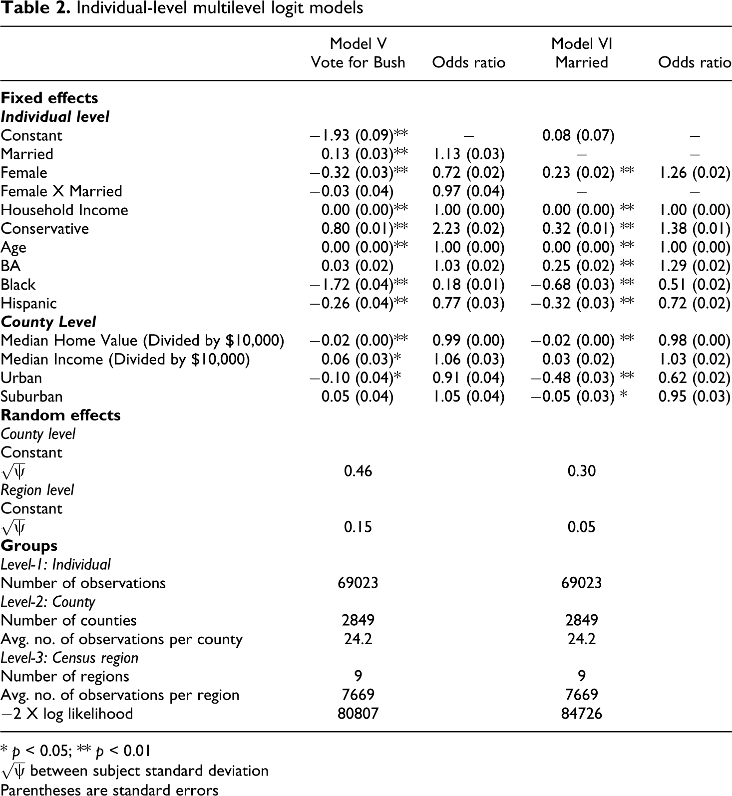
* p < 0.05; ** p < 0.01

ψ between subject standard deviation

Parentheses are standard errors

The one apparent inconsistency between the individual-level data and the aggregate-level data is the influence of education. Whereas counties with a high percentage of the population possessing a BA exhibited lower marriage rates for young women, the individual-level model shows that possessing a BA actually increased the probability that an individual would be married. This underscores the importance of exercising caution before drawing individual-level inferences from aggregate-level data. However, I must again note that the marriage variable in the aggregate models looked at only a small percentage of the total population. It is possible that possessing a BA makes it more likely that an individual will delay marriage, but actually increase the probability that an individual will get (and remain) married at some point in his or her life (Cahn and Carbone, 2010). If that is the case, the two models may not actually be inconsistent.

It is also interesting that Model V does not show any statistical significance for the interaction between gender and marriage. Although previous literature suggested that the marriage gap was stronger for women than for men, these data suggest that this was not the case in the 2000 election.

Drawing strong inferences about what was precisely causing these results is problematic. These models were the result of a single snapshot in time. I theorized that home values influence political sorting largely because they influence migratory patterns. That is, I argue that young people who formed family units at an early age also actively sought out communities in which home-ownership was not prohibitively expensive. In order to definitively confirm that this is what occurred, it is necessary to obtain more reliable data on individual-level migration patterns. Future research should examine this question in greater detail. Nonetheless, in spite of that caveat, these results suggest that the findings presented in the aggregate models were not simply the result of the ecological fallacy.