Towards a classification of the world’s democratic party systems,step 2

Abstract

This article classifies the democratic party systems of the world by using the relative-size triangle, a bounded diagram that graphically represents information about seat distributions by party. In particular, the article solves identification problems stemming from the fact that party systems, as recurring patterns of party competition, involve systemic properties that are not reducible to the properties of individual party constellations. On this basis, 162 party systems that existed or continue to exist in the world’s democracies from 1792 to 2009 are assigned to the predominant party, two-party and multiparty types, each of the types being divided into two subcategories. A new measure of party system fragmentation, the systemic effective number of parties, complements the resulting classification with a methodologically consistent assessment of the degrees of multipartism. On this basis, the article arrives at several empirical conclusions regarding the geographical/chronological spread of different party systems and their relative longevity.

Keywords

classification methodology party systems visual display

Introduction

It is traditional in political science to classify party systems by the numbers of parties. Almost sixty years ago, Ranney and Kendall (1954: 477) wrote: ‘One of the most elementary procedures used in dealing with the raw data of political conflict is that which, taking the departure from the notion of “party systems”, seeks to assign each observed instance to one or another of three types: the “one-party system”, the “two-party system”, and the “multiple-party system”’. With some minor modifications proposed by later authors, this classification remains with us today. Of course, there are many more classifications on offer in the political science marketplace. Indeed, as any complex phenomena, party systems are ‘inherently multidimensional’ (Gross and Sigelman, 1984: 463), and therefore some of the classifications simply do not involve the numbers of parties, or do so but only marginally. Such are, to cite recent examples, a classification based on the varying levels of party system institutionalization (Mainwaring, 1999) and a classification focused on the ‘open’ and ‘closed’ structures of party competition (Mair, 2002). Moreover, the classification of Sartori (1976), probably the most influential one in comparative research on party systems, is multidimensional, as it is based on at least three classificatory parameters: the number of parties, ideological distance and alternation in power.

There are several reasons for viewing the simple taxonomy that labels party system types by the numbers of parties as both viable and indispensible. First, this taxonomy is normally employed as a building block in the ongoing attempts to develop multidimensional approaches to party system classification (Wolinetz, 2006). Second, the distinction between two-party systems and multiparty systems, as well as some of the intermediate and supplementary categories, has grown to become central for several salient streams in political science research, including the interplay between electoral systems and party systems (Riker, 1982), government formation and duration (Grofman, 1989), the basic properties of different institutional designs (Shugart and Carey, 1992) and government performance (Chhibber and Nooruddin, 2004). And, last but not least, the number of parties is an intuitively appealing criterion for classifying party systems. The purpose of this article is to refine the traditional, ‘number-based’, classification of party systems in a way that will make it applicable to the whole set of the world’s democracies starting with the end of the eighteenth century. Thus the end product of the article is a party system classification that is not just a theoretical construction, but also a list of the world’s democratic party systems by category.

Feger (2001) emphasizes that before classifying individual cases, we have to answer one fundamental question: which elements are to be differentiated in a classification? Following this desideratum, Golosov (2012) proposes a set of operational criteria for identifying elements that qualify for inclusion within the universe of democratic party systems among individual election outcomes and country-specific sequences of elections. Yet, once this is done, the second step is to place the identified units into the categories of classification, which is the principal task to be solved in this analysis. The complexity of this task stems from the fact that categories are theoretical constructions, while the units of analysis are empirical phenomena, which raises the problem commonly referred to as the problem of identification: ‘We might think of identification as sticking items into pigeon holes, and classification proper as making the pigeon holes in which to stick them’ (Landa and Ghiselin, 2005: 215). Obviously, the two aspects are interrelated. That is why I start by refining an earlier proposed methodological tool (Golosov, 2011) in a way that solves the problem of identification and produces the list of party systems by category. Then, taking a more empirical perspective, I assess party system types and subtypes from the angle of their geographical and chronological spread and longevity.

Methodological issues

In this study, I use an earlier introduced methodological tool for party system classification dubbed the relative-size triangle (RST). This tool, building on the tradition of number-based classifications as represented by Blondel (1968), Ware (1996) and Siaroff (2000), and informed by important contributions of Sartori (1976), Laakso and Taagepera (1979) and Grofman et al. (2004), is discussed in detail elsewhere (Golosov, 2011). The minimum of necessary information can be summarized thus. The word ‘triangle’ refers to the fact that the first step in this classification procedure is a two-dimensional graphical representation, with individual party constellations being entered as data points with the following coordinates:

x = \frac{s_{2} + s_{r}}{s_{1} + s_{r}}

y = \frac{s_{3} + s_{r}}{s_{1} + s_{r}}

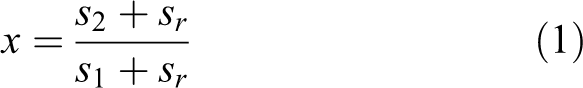
Here, s ₁, s ₂ and s ₃ are percentage shares of legislative seats taken by the top, second-largest and third-largest parties, respectively, whereas s_r is the share of seats jointly received by all parties from the fourth-largest to the smallest.

Figure 1 shows the resulting graphical representation. The feasible set of data points lies within a triangle, the bounds of which are the x-axis (AC), the x = 1 line (BC) and the y = x line (AB). The medians divide the triangle into six equal-size segments corresponding to the theoretically important types of party systems. In order to define these segments in substantive terms, we have to look at the equations describing the medians of the triangle, which are y = 0.5x for AF, y = 1 – x for CE and y = 2x – 1 for BD. These equations can be redefined in terms of the sizes of the components. The y = 1 – x equation rewrites as s₁ = s₂ + s₃ + s_r , which can be achieved only if s₁ = 0.5. Then all data points lying below the CE line represent those constellations in which there is a majority party, the points above it, those in which there is not, and the points on it, those where the majority party takes exactly half of the seats. The similarly constructed equation for the AF line is s₃ = (s₂ – s_r ) / 2 and for the BD line, s₂ = (s₁ + s₃ ) / 2. The relationships between some of the segments of the diagram and the major types identified in traditional typologies are not problematic, because they are defined by the vertices of the triangle. The A vertex represents the constellation in which all seats are taken by one party, which is perfect one-party dominance. All other points along the AC line represent two-component constellations. Of them, the C vertex is the point of perfect bipartism, because here there are two equal-size parties. At the vertex B, we find perfect multipartism, with constellations of more than two equal-size parties. Then the quadrangular regions taking a third of the available space each, ADEG, CDFG and BEFG, represent the predominant-party, two-party and multiparty constellations, respectively. Each of them is divided by the segments of the median lines into two equal-size areas corresponding to party system subtypes: polyvalent (AEG) and bivalent (ADG) predominant-party systems; monovalent (CDG) and polyvalent (CFG) two-party systems; and bivalent (BFG) and monovalent (BEG) multiparty systems. The former is the one in which the largest party is at a strong advantage over all others, including the closest challenger, while in the latter there is little distance between the two largest parties. The monovalent two-party system is the two-party system in the traditional sense, while the polyvalent two-party system is very close to the two-and-a-half party system type. The literature does not draw a distinction between the polyvalent and monovalent predominant-party systems, but for those scholars who do not single out the type as such, systems with many comparably small challengers normally fall into the category of multipartism, while systems where there is only one visible challenger, into the category of bipartism.

Figure 1.

The segmented relative size triangle with some data points of significance.

Being focused on relative imbalances among the leading parties, the RST does not measure party system fragmentation, for which purpose the effective number of parties (Golosov, 2010; Laakso and Taagepera, 1979) remains indispensible. It would be incorrect, however, to assume that the fragmentation aspect is completely unaddressed by the proposed method. It is incorporated by using the s_r term in formulae (1) and (2). In the mathematical construction of the RST, the values of s_r are the theoretical limits of x and y values. For instance, no constellation in which minor parties, starting with the fourth one, jointly take 50 percent of seats, can be placed below the EF line on the diagram irrespective of the absolute sizes of the components, which promptly characterizes such constellations as different from those with limited minor party presence. In practice, the use of the s_r term greatly increases the applicability of the RST diagram to the analysis of constellations with more than three parties.

At the most easily available level of observation, party systems manifest themselves as election outcomes, and some of the commonly used tools of party system measurement are adjusted to the level of individual elections. The effective number of parties can be calculated for each of them. For Siaroff (2000), a national party system can be identified and categorized already on the basis of a single legislative election. However, this approach is scarcely consistent with the theoretical notion of party systems as recurring patterns of interaction among political parties (Sartori, 1976), because this definition explicitly involves cross-temporal continuity as an essential party system property. Thus the adequate empirical referent for a party system is a sequence of elections, not an individual election. Moreover, even sequences of elections are not necessarily manifestations of party systems, because some of them do not display any recurrent patterns. Building on these premises, Golosov (2012) introduces and explains in detail a set of operational criteria for identifying elements that qualify for inclusion within the universe of democratic party systems. These elements are sequences of no less than three national legislative elections held in the course of five or more years. In order to qualify, the elections are to be held in independent countries, in democratic conditions and return party-structured legislatures. Some of the sequences of elections that meet these criteria serve as carriers for single party systems, while others either fall into the category of party non-systems (Sanchez, 2009) or can be divided into several units. The criteria used for differentiating among party systems and party non-systems, and for drawing lines between individual party systems within national settings, are extra-system volatility of no less than 25 percent¹ and cumulative party system change measured by the dynamics in party system fragmentation. By applying these criteria to a set of 1502 national legislative elections held in the world’s democracies from 1792 to 2009, Golosov (2012) identifies 162 units that can be entered into a classification of the world’s democratic party systems and 21 party non-systems.²

This is the point of departure for identification problems. With the list of units for analysis and the method of classification at hand, the task is to place the units within categories, which requires adjusting the methods developed for individual elections to the level of election sequences. For a long time, this requirement remained unrecognized because an obvious solution seemed to be available. Blondel (1968), whose classificatory criterion was the joint share of the vote cast for the two leading parties, simply averaged them for the whole period of observation. Similarly, Siaroff (2000) employs the median values of the seat-shares won by the first, second and third-largest parties. In studies employing the effective number of parties, taking averages of the values calculated for individual election outcomes is a standard procedure (Lijphart, 1994). Golosov (2011), in his illustrative application of the relative-size triangle to a set of post-World War II democracies, locates party systems at data points with the median x and y coordinates. But this procedure, even if standard, is profoundly flawed, which is immediately apparent from the following example. The example is hypothetical, but the situation described in it is rather usual, being quite widespread, for instance, in the small democracies of the Caribbean. Consider a sequence of four elections with only two parties gaining representation. In the first election, the absolute share of seats gained by party A is 0.9 and by party B, 0.1; the subsequent seat-shares of the respective parties are (0.2, 0.8), (0.7, 0.3), and (0.0, 1.0). In this sequence, the average/median share of seats taken by the largest party is 0.85, while the second party takes 0.15, which obviously characterizes the party system as belonging to the predominant-party type. The average and median effective numbers of parties are 1.20 and 1.18, respectively.³ Is this really a predominant-party system?

The reason why we are unwilling to answer this question positively is that we observe a perfect pattern of alternation in power, which is indeed a criterion introduced by Sartori (1976) for distinguishing between this type and the category of two-party systems. Does this mean that a party system classification based on simple numerical criteria is, after all, infeasible? No, but it is necessary to find a way of quantifying the notion of alternation in power on the basis of seat distributions. The example of the preceding paragraph is simplistic enough to make this way apparent. In two-party systems, such as in this example, there is always a majority party. The inadequate quantifications cited above are all based on an implicit assumption that there is only one majority party throughout the entire sequence of elections. But in fact there are two parties alternating in the leading position. In order to take this into account, it is sufficient to use a different basis for taking averages by calculating them not for whole constellations but for individual parties. In the example, the average share of seats gained by party A across four elections is 0.45, and by party B 0.55. This makes for a two-party system by any method using numerical criteria. But if there were indeed only one majority party throughout the sequence of elections, then, with the same seat distributions in individual constellations, a predominant-party system would be in place.

The solution proposed here is situational, but it is theoretically justifiable. From a macro-theoretical perspective, averaging individual-level values does not necessarily lead us to revealing systemic properties because a system, by definition, is not equivalent to an aggregate of its components (Von Bertalanffy, 1968). Correspondingly, the systemic properties can be different from the properties established for individual-level observations. In the above-cited example, four constellations obviously belonging to the predominant-party type fuse to create a party system of the two-party type. From the perspective of the general theory of party systems (Sartori, 1976), cross-temporal continuities and discontinuities in the strength of individual parties are essential for establishing the patterns of interaction among them, without which our empirically informed vision of party systems would be void.

Turning to a more methodological level of discussion, the proposed way of placing the individual party system units within categories is thus: First, calculate the average share of seats gained by each of the parties for the entire sequence of elections, irrespective of their number.⁴ Second, sort the averages by size, which establishes the values of s ₁, s ₂, s ₃ and s_r . Then use the formulae (1) and (2), as defined above, to establish the RST data point for each of the party systems, further referred to as their systemic locations. The segment of the RST inside which the data point falls assigns the party system to this or that category. In this respect, a minor clarification is in order. It takes an effort to establish continuities between individual parties, because they change labels over time, and especially between parties and coalitions. This effort, however, is not a part of solving the problem of identification per se, but rather a necessary condition for disaggregating large sequences of elections into units corresponding to individual party systems, for which the criterion of extra-system volatility is indispensable. It can be argued that the proposed method allows for integrating, both at theoretical and empirical levels, party system classification with the ongoing research on party system volatility, a fundamental party system property by any account. In particular, this flourishing field provides technical solutions to many issues related to tracing continuities among parties (Sikk, 2005). One might argue that averaging election results for individual parties does not reveal consistent patterns because some of the party systems are volatile. This argument could be convincing if, when identifying the units for analysis, no distinctions were drawn between party systems and non-systems, and among individual party systems within larger sequences of elections. But in practice the use of adequate operational criteria for identifying the units of analysis (Golosov, 2012) eliminates this problem. Using a set of the real-life data, Figure 2 shows how the systemic locations of six party systems, selected to represent different party system types, relate to the RST locations of individual election outcomes.

Figure 2.

The RST locations of six party systems and individual election outcomes, 1938–2009.*

As mentioned above, the merits of the RST display do not include precision in differentiating party systems by the levels of fragmentation. This is immediately apparent from the fact that all constellations consisting of equal-size components, irrespective of their numbers, fall into the B vertex of the diagram. A possible solution for this problem can be a quasi-three-dimensional graphical display with the third dimension expressing fragmentation, but precision in data representation would be insufficient. A better solution is to use the effective number of parties as a supplementary measure. The methodological problem here is how to count it. While the standard method is to take averages of the numbers calculated for individual constellations, a better solution can be derived from reasoning above. Since establishing the RST locations for party systems already involves cross-temporal averaging of individual parties’ seat-shares, the resulting averages, always summing up to 1.0, can be used for calculating the effective number of parties. I dub this measure the ‘systemic effective number of parties’ (SENP). The formula for the SENP is the same as for the standard effective number of parties (see note 4), but s_i and s₁ are redefined as in the procedure described at the beginning of the previous paragraph. The values of the SENP are normally (but not necessarily) greater than those of the average effective number of parties. In the above-cited hypothetical sequence with the seat-shares of (0.9, 0.1), (0.2, 0.8), (0.7, 0.3) and (0.0, 1.0), the average effective number of parties is 1.20, which obviously does not tell much about this party system, and the SENP is 1.82, which properly describes it as a case of bipartism.

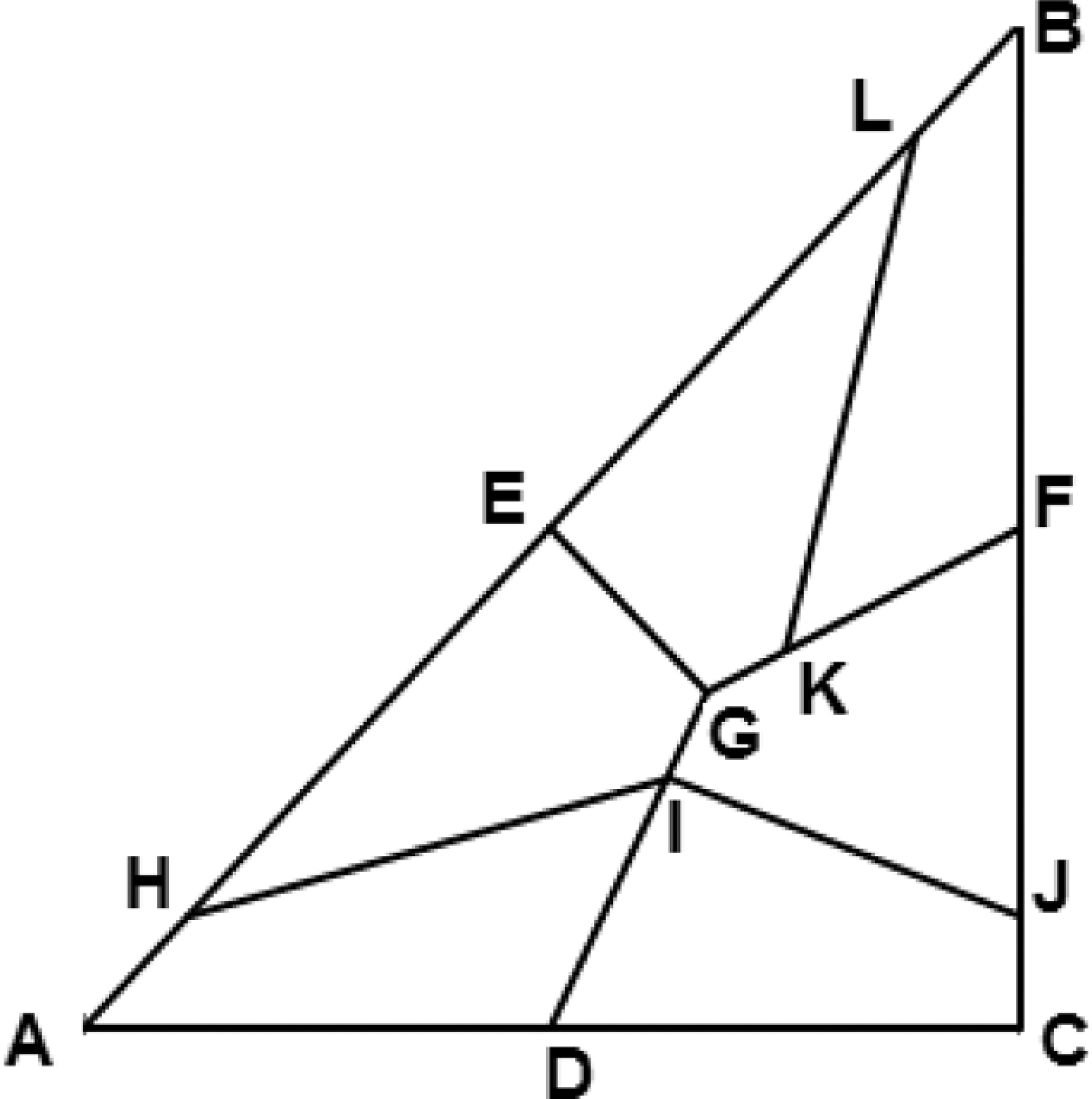
This is not to say that the transition from the RST placement of individual election outcomes to the identification of party system locations by the proposed method is absolutely unproblematic. Consider a hypothetical sequence of three elections with three parties, A, B and C, receiving the respective shares of legislative seats of (0.57, 0.40, 0.03), (0.25, 0.72, 0.03) and (0.62, 0.35, 0.03). Parties A and B alternate in power, while party C is very small and obviously lacks significant influence. Yet the average shares of seats are 0.48 (A), 0.49 (B) and 0.03 (C), which places the system within the polyvalent two-party category (S on Figure 1). For an individual election outcome, such a placement would be entirely justifiable given the clearly manifested coalition potential of the party C, but at the systemic level no such potential is evident. In order to provide for a more adequate categorization, I modified the segmentation of the RST originally proposed by Golosov (2011) by removing the small CLM area immediately adjacent to the point of perfect bipartism from the category of polyvalent two-party systems, and reassigned it to the category of monovalent two-party systems. The line is drawn in a way that roughly corresponds to Siaroff’s (2000) idea of using the median 95 percent two-party concentration as a cut-off point between two-party systems and two-and-a-half party systems. The exact coordinates of the L and M data points are (1.0, 0.102) and (0.898, 0.102), which, for a three-party constellation with two large equal-size parties, corresponds to the 4.86 percent seat-share of the smallest party and to the 95.14 percent two-party concentration.

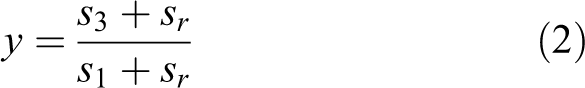
Then I proceeded to redefine other party system subtypes. There were two substantive reasons for this. First, as Grofman et al. (2004) correctly suggest, for a graphical presentation of this kind to be efficient it has to allocate equal regions to all theoretically important types. But, with the relocation of the CLM segment, this requirement was no longer satisfied. Second, it was clear from the very beginning that at the RST data points located closely to the vertices and the centroid of the triangle (G), the distinctions among party system subtypes are blurred. For example, the constellation (0.35, 0.325, 0.325) falls into the monovalent multiparty category (T on Figure 1), but the distance between the leading party and the two smaller parties is negligible, which clearly puts such a categorization in question. In fact, it is more realistic to view it as a balanced constellation, with the sizes of the three parties being almost equal. Similarly, the constellation (0.52, 0.34, 0.14) is within the monovalent two-party category (U on Figure 1), but the size of the smallest party is such that the polyvalent subtype is, intuitively, a more likely placement. Then, leaving the boundaries between party system types intact, I redefine party system subtypes. Within the ADEG quadrangle, the AHI segment is assigned to the bivalent predominant-party subtype, and the GON segment to the polyvalent predominant-party subtype; within the CDFG quadrangle, the CLM segment goes to the monovalent two-party subtype, and the GOP segment to the polyvalent two-party subtype; and within the BEFG quadrangle, the BJK segment is now in the bivalent multiparty category, while the GQR segment is in the monovalent multiparty category.⁵ In the resulting graphical display, the regions allocated to each of the subtypes remain equal; the scope of change is very limited, as the relocated segments jointly take only 6.25 percent of the area of the triangle; and the symmetry pattern of the previous segmentation is retained. The newly introduced segmentation lines can be defined in terms of the relative sizes of components by a set of easy-to-use, intuitively appealing, equations. For instance, the QR line (x = 0.75) is alternatively described by the equation s₂ = 0.75s₁ – 0.25s_r . Figure 3 shows the RST diagram with the new segmentation.⁶

Figure 3.

The RST display with the reformulated definitions of segments.

Empirical perspectives

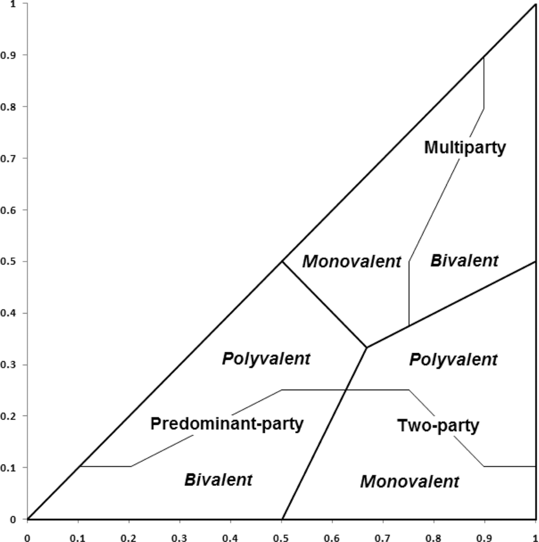
Overall, the resulting classification of the world’s democratic party systems includes 162 units. Of these, 31 are predominant-party systems, 61 are two-party systems and 70 are multiparty systems. The mean and median values of the SENP for each of the categories are reported in Table 1. As follows from the data, in a very broad sense the effective number of parties approach is consistent with the fundamental premises of the number-based classification of party systems, as the SENP increases in a curvilinear fashion from single-party predominance to multipartism. However, a more nuanced picture emerges from Table 2 that reports the values of the SENP for party system subtypes. Here, the dynamics of the SENP is not curvilinear but rather cyclical: starting with 1.44 (bivalent predominant-party systems), the average SENP grows to achieve its apex for the bivalent multiparty system subtype, and then decreases, starting with monovalent multipartism, to the category of predominant-party systems, of which the polyvalent subtype is less concentrated than the bivalent one. The lack of linear relationship between the effective number of parties and party system categories is especially evident from the ranges of the SENP values reported in Tables 1 and 2. This finding promises a methodological improvement for the streams of research that use the effective number of parties, taken as a proxy for party system type, as a dependent variable (which is common, for instance, in the study of electoral system effects). It is quite possible that different – and more precise – research results can be obtained by operationalizing party system types/subtypes as explicitly defined, mutually exclusive categories, not by proxy. Of course, further discussion of this issue is beyond the scope of this inquiry.

Table 1.

The world’s democratic party systems by type, 1792–2009.

Party system type	n	Mean SENP	Median SENP	Range, SENP
Predominant-party	31	1.61	1.52	1.04–2.34
Two-party	61	2.29	2.28	1.76–3.40
Multiparty	70	4.36	3.70	2.31–11.85

Table 2.

The world's democratic party systems by subtype, 1792-2009.

Party system subtype	n	Mean SENP	Median SENP	Range, SENP
Polyvalent predominant-party	18	1.74	1.62	1.29–2.34
Bivalent predominant-party	13	1.44	1.43	1.04–1.99
Monovalent two-party	26	1.93	1.93	1.76–2.11
Polyvalent two-party	35	2.56	2.44	2.18–3.40
Bivalent multiparty	42	4.86	4.23	2.31–11.85
Monovalent multiparty	28	3.62	3.22	2.34–6.27

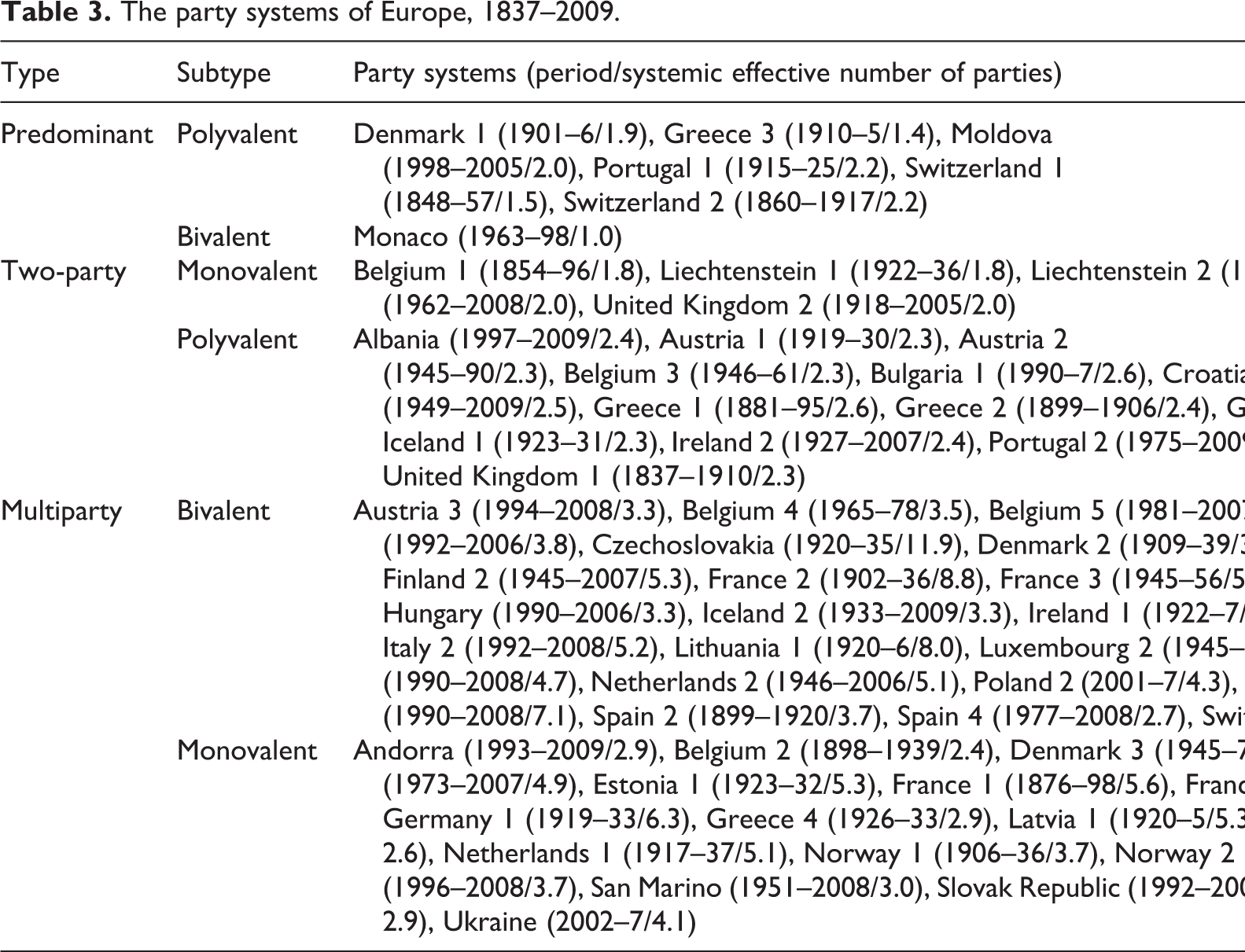
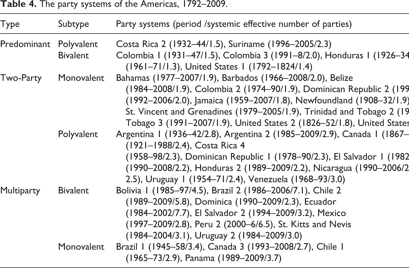
In a diagram form, the classification of the world’s democratic party systems is given in Figures 4 –6, supplemented with Tables 3 – 5. The tables also report the SENP values and the chronological limits for each of the systems, defined by the earliest and most recent elections as of 2009.⁷ The black data points correspond to those party systems that remained in place by the end of 2009, while the white ones, to those that became extinct. I represent party systems by broadly defined geographical region simply to make the diagrams more readable, but it also forms a suitable basis for a brief discussion below. Indeed, geographical regions display divergent patterns of party systems. Europe, as follows from Figure 4, is the true home of multipartism. It was always a prevailing type. Polyvalent predominant-party systems did exist in the past, and one of them resurfaced recently (Moldova), but by 2009 all of them were gone. The bivalent predominant-party type is virtually absent, while monovalent two-party systems are few, including, in addition to the United Kingdom and Malta, only the first party system of Belgium, as well as Liechtenstein. Bipartism is represented mostly by the polyvalent subtype, but this subtype, even with the archetypical case of Germany, is not densely populated either.

Figure 4.

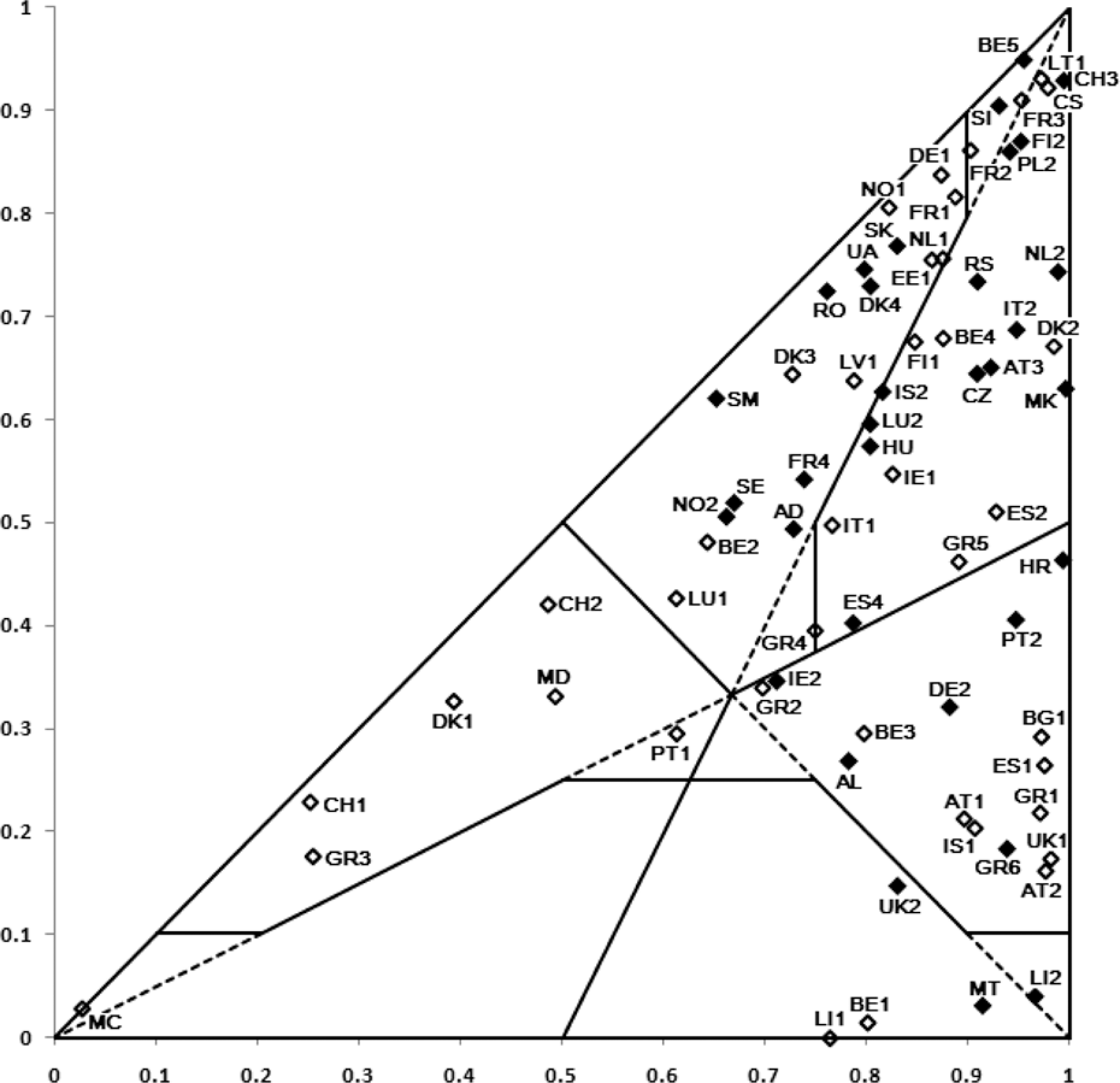
The party systems of Europe, 1837–2009.

Figure 5.

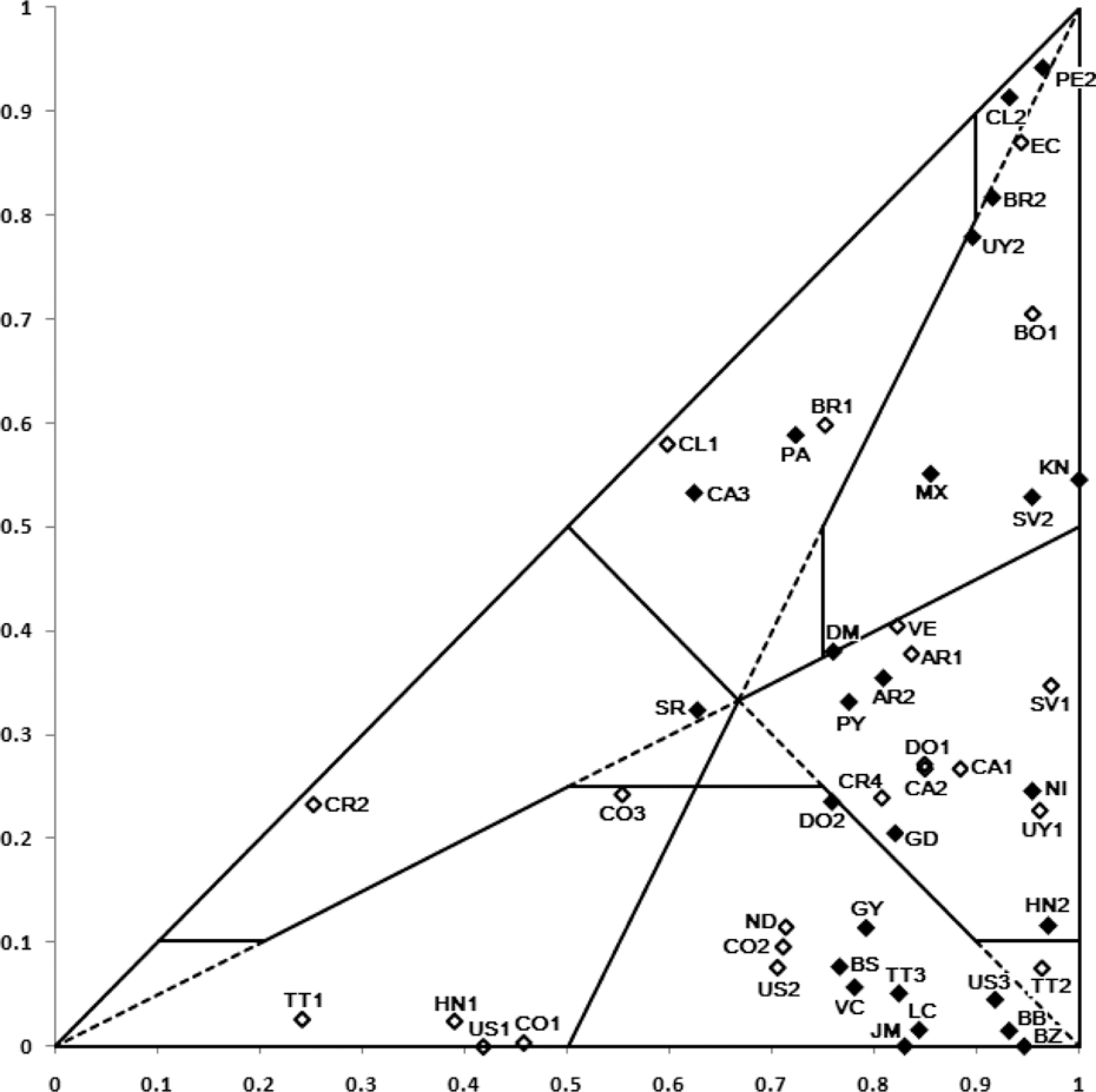
The party systems of the Americas, 1792–2009.

Figure 6.

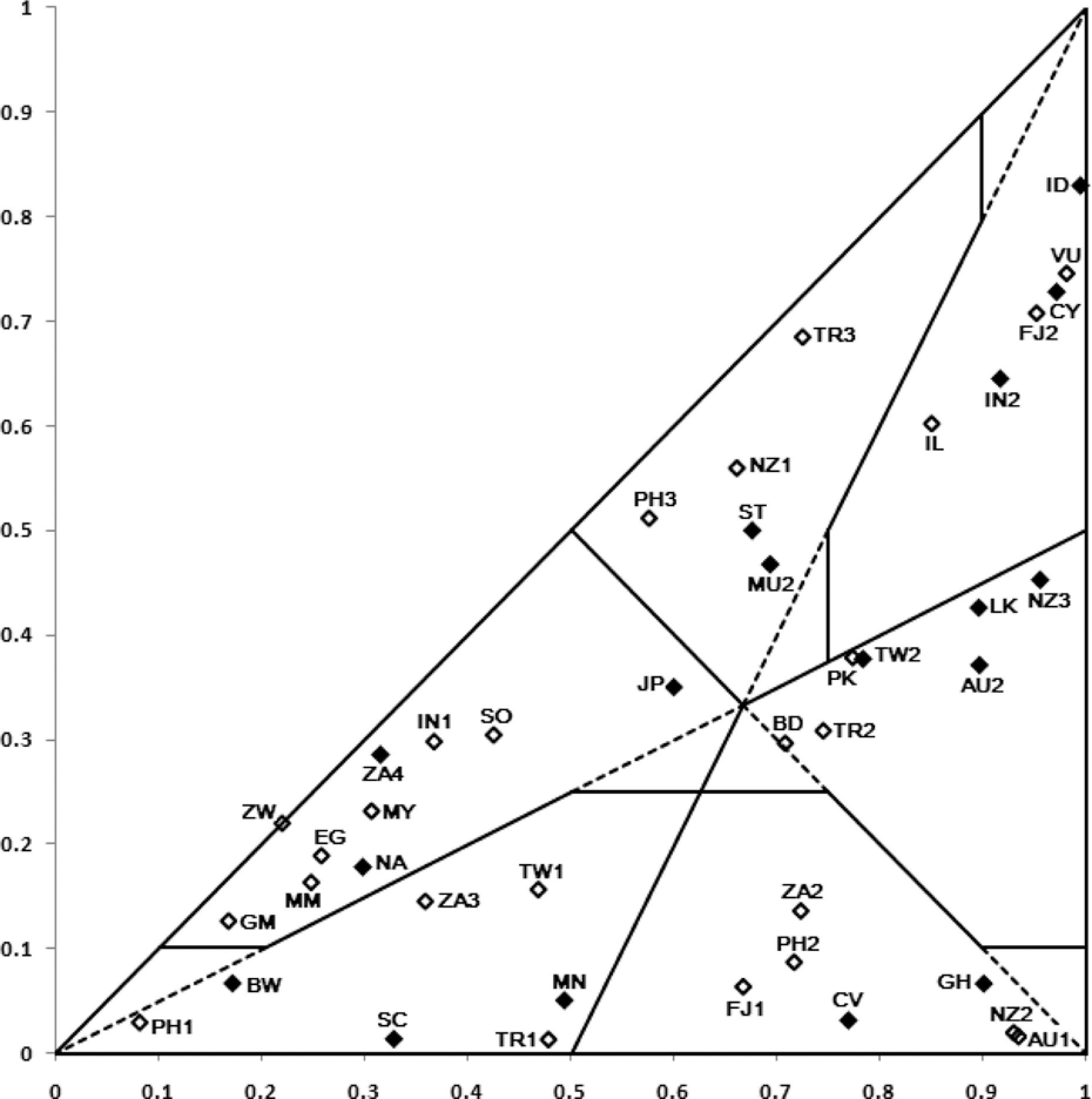
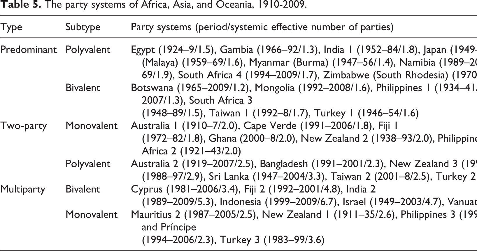
The party systems of Africa, Asia and Oceania, 1921–2009.

Table 3.

The party systems of Europe, 1837–2009.

Type	Subtype	Party systems (period/systemic effective number of parties)
Predominant	Polyvalent	Denmark 1 (1901–6/1.9), Greece 3 (1910–5/1.4), Moldova (1998–2005/2.0), Portugal 1 (1915–25/2.2), Switzerland 1 (1848–57/1.5), Switzerland 2 (1860–1917/2.2)
Predominant	Bivalent	Monaco (1963–98/1.0)
Two-party	Monovalent	Belgium 1 (1854–96/1.8), Liechtenstein 1 (1922–36/1.8), Liechtenstein 2 (1945–2009/2.0), Malta (1962–2008/2.0), United Kingdom 2 (1918–2005/2.0)
Two-party	Polyvalent	Albania (1997–2009/2.4), Austria 1 (1919–30/2.3), Austria 2 (1945–90/2.3), Belgium 3 (1946–61/2.3), Bulgaria 1 (1990–7/2.6), Croatia (2000–7/3.4), Germany 2 (1949–2009/2.5), Greece 1 (1881–95/2.6), Greece 2 (1899–1906/2.4), Greece 6 (1974–2009/2.4), Iceland 1 (1923–31/2.3), Ireland 2 (1927–2007/2.4), Portugal 2 (1975–2009/2.8), Spain 1 (1879–98/2.7), United Kingdom 1 (1837–1910/2.3)
Multiparty	Bivalent	Austria 3 (1994–2008/3.3), Belgium 4 (1965–78/3.5), Belgium 5 (1981–2007/10.2), Czech Republic (1992–2006/3.8), Czechoslovakia (1920–35/11.9), Denmark 2 (1909–39/3.6), Finland 1 (1919–39/3.7), Finland 2 (1945–2007/5.3), France 2 (1902–36/8.8), France 3 (1945–56/5.2), Greece 5 (1950–64/3.1), Hungary (1990–2006/3.3), Iceland 2 (1933–2009/3.3), Ireland 1 (1922–7/3.4), Italy 1 (1946–87/3.0), Italy 2 (1992–2008/5.2), Lithuania 1 (1920–6/8.0), Luxembourg 2 (1945–2009/3.1), Macedonia (1990–2008/4.7), Netherlands 2 (1946–2006/5.1), Poland 2 (2001–7/4.3), Serbia (2003–8/4.1), Slovenia (1990–2008/7.1), Spain 2 (1899–1920/3.7), Spain 4 (1977–2008/2.7), Switzerland 3 (1919–2007/5.4)
Multiparty	Monovalent	Andorra (1993–2009/2.9), Belgium 2 (1898–1939/2.4), Denmark 3 (1945–71/3.6), Denmark 4 (1973–2007/4.9), Estonia 1 (1923–32/5.3), France 1 (1876–98/5.6), France 4 (1958–2007/3.0), Germany 1 (1919–33/6.3), Greece 4 (1926–33/2.9), Latvia 1 (1920–5/5.3), Luxembourg 1 (1919–37/2.6), Netherlands 1 (1917–37/5.1), Norway 1 (1906–36/3.7), Norway 2 (1945–2009/2.9), Romania (1996–2008/3.7), San Marino (1951–2008/3.0), Slovak Republic (1992–2006/4.7), Sweden (1911–2006/2.9), Ukraine (2002–7/4.1)

Table 4.

The party systems of the Americas, 1792–2009.

Type	Subtype	Party systems (period /systemic effective number of parties)
Predominant	Polyvalent	Costa Rica 2 (1932–44/1.5), Suriname (1996–2005/2.3)
Predominant	Bivalent	Colombia 1 (1931–47/1.5), Colombia 3 (1991–8/2.0), Honduras 1 (1926–34/1.4), Trinidad and Tobago 1 (1961–71/1.3), United States 1 (1792–1824/1.4)
Two-Party	Monovalent	Bahamas (1977–2007/1.9), Barbados (1966–2008/2.0), Belize (1984–2008/1.9), Colombia 2 (1974–90/1.9), Dominican Republic 2 (1998–2006/2.1), Guyana (1992–2006/2.0), Jamaica (1959–2007/1.8), Newfoundland (1908–32/1.9), St. Lucia (1979–2006/1.9), St. Vincent and Grenadines (1979–2005/1.9), Trinidad and Tobago 2 (1976–86/2.1), Trinidad and Tobago 3 (1991–2007/1.9), United States 2 (1826–52/1.8), United States 3 (1854–2008/2.0)
Two-Party	Polyvalent	Argentina 1 (1936–42/2.8), Argentina 2 (1985–2009/2.9), Canada 1 (1867–1917/2.4), Canada 2 (1921–1988/2.4), Costa Rica 4 (1958–98/2.3), Dominican Republic 1 (1978–90/2.3), El Salvador 1 (1982–91/2.6), Grenada (1990–2008/2.2), Honduras 2 (1989–2009/2.2), Nicaragua (1990–2006/2.5), Paraguay (1993–2008/2.5), Uruguay 1 (1954–71/2.4), Venezuela (1968–93/3.0)
Multiparty	Bivalent	Bolivia 1 (1985–97/4.5), Brazil 2 (1986–2006/7.1), Chile 2 (1989–2009/5.8), Dominica (1990–2009/2.3), Ecuador (1984–2002/7.7), El Salvador 2 (1994–2009/3.2), Mexico (1997–2009/2.8), Peru 2 (2000–6/6.5), St. Kitts and Nevis (1984–2004/3.1), Uruguay 2 (1984–2009/3.0)
Multiparty	Monovalent	Brazil 1 (1945–58/3.4), Canada 3 (1993–2008/2.7), Chile 1 (1965–73/2.9), Panama (1989–2009/3.7)

Table 5.

The party systems of Africa, Asia, and Oceania, 1910-2009.

Type	Subtype	Party systems (period/systemic effective number of parties)
Predominant	Polyvalent	Egypt (1924–9/1.5), Gambia (1966–92/1.3), India 1 (1952–84/1.8), Japan (1949–2009/2.3), Malaysia (Malaya) (1959–69/1.6), Myanmar (Burma) (1947–56/1.4), Namibia (1989–2009/1.5), Somalia (1959–69/1.9), South Africa 4 (1994–2009/1.7), Zimbabwe (South Rhodesia) (1970–7/1.4)
Predominant	Bivalent	Botswana (1965–2009/1.2), Mongolia (1992–2008/1.6), Philippines 1 (1934–41/1.1), Seychelles (1998–2007/1.3), South Africa 3 (1948–89/1.5), Taiwan 1 (1992–8/1.7), Turkey 1 (1946–54/1.6)
Two-party	Monovalent	Australia 1 (1910–7/2.0), Cape Verde (1991–2006/1.8), Fiji 1 (1972–82/1.8), Ghana (2000–8/2.0), New Zealand 2 (1938–93/2.0), Philippines 2 (1949–65/1.9), South Africa 2 (1921–43/2.0)
Two-party	Polyvalent	Australia 2 (1919–2007/2.5), Bangladesh (1991–2001/2.3), New Zealand 3 (1996–2008/3.3), Pakistan (1988–97/2.9), Sri Lanka (1947–2004/3.3), Taiwan 2 (2001–8/2.5), Turkey 2 (1961–9/2.4)
Multiparty	Bivalent	Cyprus (1981–2006/3.4), Fiji 2 (1992–2001/4.8), India 2 (1989–2009/5.3), Indonesia (1999–2009/6.7), Israel (1949–2003/4.7), Vanuatu (1991–2002/4.2)
Multiparty	Monovalent	Mauritius 2 (1987–2005/2.5), New Zealand 1 (1911–35/2.6), Philippines 3 (1995–2001/2.9), São Tomé and Príncipe (1994–2006/2.3), Turkey 3 (1983–99/3.6)

In contrast, the party systems of the Americas are characterized by a widespread presence of bipartism in both varieties. The monovalent two-party segment is populated mostly with English-speaking countries, from the United States to the bulk of the small democracies of the Caribbean. Among the polyvalent two-party systems, we find quite a lot of Latin American countries with a noticeable addition of the old party systems of Canada, but many party systems in this segment are extinct. This corresponds to the Latin American trend towards multipartism described by Mainwaring (1999). Even with this trend, however, Latin America does not match Europe in the spread of multipartism. Predominant-party systems in the Americas are few, almost completely extinct, and represented mostly by the bivalent subtype. In general, the picture of the party systems of the Americas is clearly biased towards the right side of the RST diagram, which indicates closeness of competition between the largest parties.

The party systems of Africa, Asia and Oceania display a less consistent pattern, which is obviously connected to the scope and diversity of the region. However, it is quite clear that the likelihood of predominant-party systems in this region is a lot higher than in the previous cases. They can be met not only in Africa, where they are indeed widespread (Bogaards, 2004), but also in Asia, and not just among the extinct party systems, but also among the existing ones. Thus each of the geographical regions has a characteristic party system type, even though the populations of all regions are diverse. The log-linear analysis of the distributions represented in Figures 4 –6 (not reported here) confirmed this observation, but it is noticeable that with the RST the association between regions and party system types is apparent without using sophisticated statistical techniques. This property of the diagram can be utilized when pursuing much more delicate research agendas.

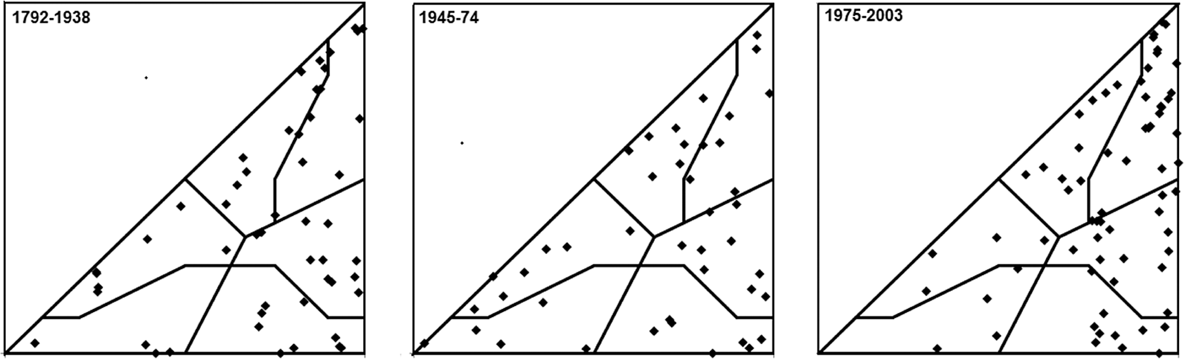
The chronological distribution of party system types and subtypes is much more even than their geographical distribution. The relevant information is reported in Tables 6 and 7. Here, party systems are classified by the time of their emergence, registered as the year of the earliest election in the corresponding sequence. When choosing a proper periodization of the global process of party system development, I sought to relate it to the notion of the three ‘waves of democratization’ (Hungtington, 1991), but at the same time to adjust it to the peculiarities of the phenomena under observation. The period from 1792 to 1938 roughly corresponds to Huntington’s ‘first wave’ and the subsequent democratic recession. As no new party systems arrived in 1939–44, the next period starts with 1945 and, embracing the second wave in its entirety, ends in 1974. I begin the ongoing third wave with 1975 because its opening event, the 1974 Portuguese revolution, spanned the first democratic election only in the subsequent year. Consistently with the method of identifying the units of analysis, no new party systems were registered after 2003. As follows from Table 6, the share of two-party systems remained stable through all three waves of democratization. The share of multiparty systems markedly increased in the third wave, which corresponds to the declining share of predominant-party systems. However, Table 7 demonstrates that if party system subtypes are taken into account, the 1975–2003 expansion of multipartism can be effectively reduced to the spread of bivalent multiparty systems, while the share of monovalent multiparty systems slightly declined. In general, the findings suggest that the most recent global trend in party system development was not towards fragmentation, as quite a number of new two-party systems emerged, but rather towards closeness of competition among the largest parties. This resulted in the declining shares of less competitive systems, not only predominant-party but also monovalent multiparty. Figure 7 provides a visual confirmation to this conclusion. Note that the locations of systems with the closest competition between the first and second-largest parties are close to the vertical axis. At the same time, the graphical display clearly suggests that the chronological patterns in party system development are not very salient.

Table 6.

The types of the world’s democratic party systems by the time of emergence, 1792–2003 (percentage shares; numbers in parentheses).

Party system type	1792–1938	1945–74	1975–2003
Predominant-party	21.57 (11)	27.91 (12)	11.76 (8)
Two-party	39.22 (20)	37.21 (16)	36.76 (25)
Multiparty	39.22 (20)	34.88 (15)	51.47 (35)
Total	100.01* (51)	100.0 (43)	99.99* (68)

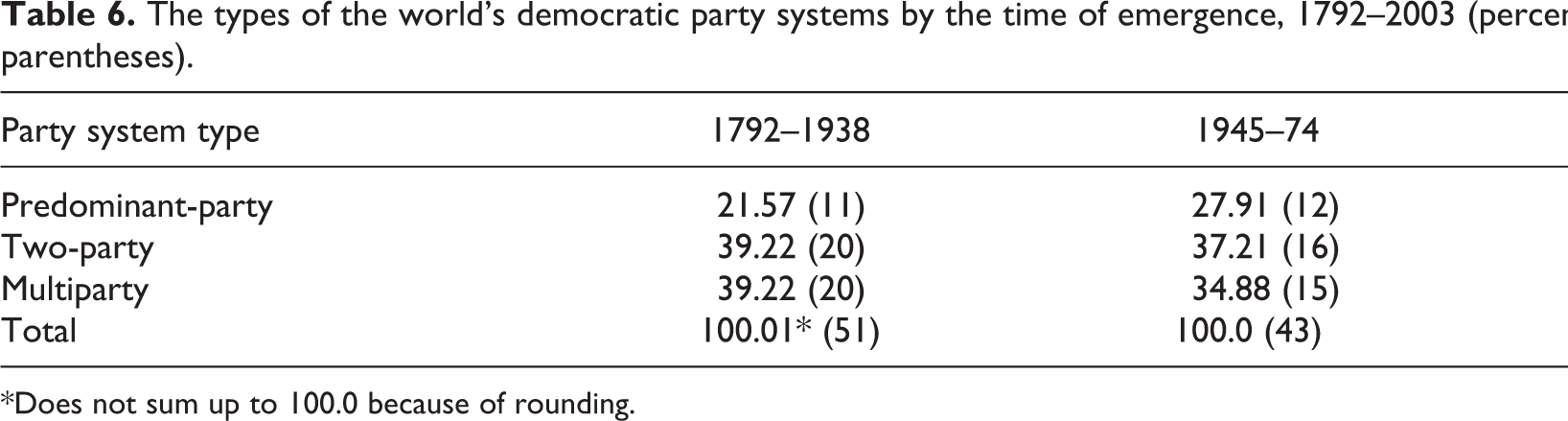
*Does not sum up to 100.0 because of rounding.

Table 7.

The subtypes of the world’s democratic party systems by the time of emergence, 1792–2003 (percentage shares; numbers in parentheses).

Party system subtype	1792–1938	1945–74	1975–2003
Polyvalent predominant-party	13.73 (7)	16.28 (7)	5.88 (4)
Bivalent predominant-party	7.84 (4)	11.63 (5)	5.88 (4)
Monovalent two-party	17.65 (9)	16.28 (7)	14.71 (10)
Polyvalent two-party	21.57 (11)	20.93 (9)	22.06 (15)
Bivalent multiparty	17.65 (9)	18.60 (8)	36.76 (25)
Monovalent multiparty	21.57 (11)	16.28 (7)	14.71 (10)
Total	100.01* (51)	100.0 (43)	100.0 (68)

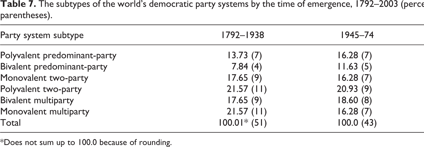
*Does not sum up to 100.0 because of rounding.

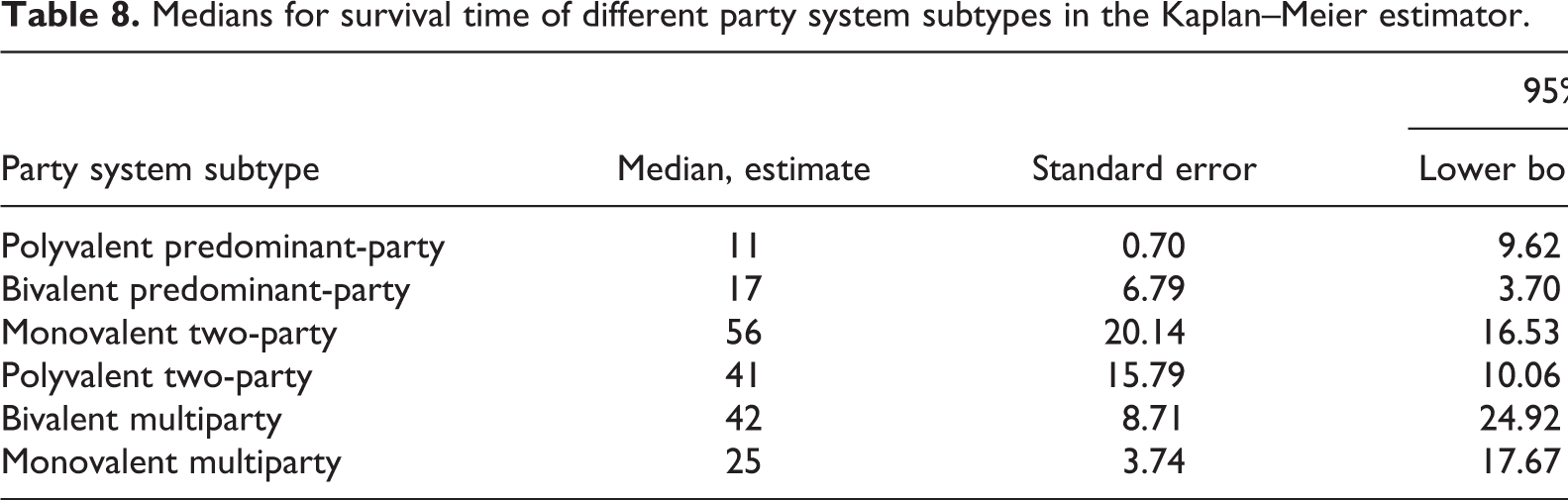
The final empirical perspective to be taken in this study is on party system longevity. Which party systems are more durable? This question cannot be answered by simply calculating their average periods of existence, because many of them have been in place at the time of observation, and their ultimate longevity is unknown. Fortunately, the Kaplan–Meier estimator, which has long been established as a standard procedure in survival analysis (Cox and Oakes, 1984), can be employed for solving such problems, as it is developed specifically for dealing with the censored data. Table 8 reports the medians for survival time of different party system types in the Kaplan–Meier estimator. As follows from the table, monovalent two-party systems are most durable, with the median estimated survival time of 56 years. They are followed by polyvalent two-party systems and bivalent multiparty systems, and distantly traced by monovalent multiparty systems and the two varieties of single-party dominance. A more nuanced picture emerges from Figure 8 that plots the Kaplan–Meier estimates of the survival functions for six party system subtypes. As is evident, the survival trajectories of different party systems are divergent from the outset, but the patterns vary over time. In the course of the first 20 years, the probability of survival is highest for monovalent two-party systems and bivalent multiparty systems. They are followed by polyvalent two-party systems and monovalent multipartism. Then the probability of survival of the party systems belonging to the latter subtype declines, and after approximately 30 years they become a part of the same group as predominant-party systems that consistently demonstrate low longevity. At the same time, polyvalent bipartism starts to display a pattern similar to those of the most durable party systems.

Figure 7.

The world's democratic party systems by the period of their emergence, 1792–2003.

Figure 8.

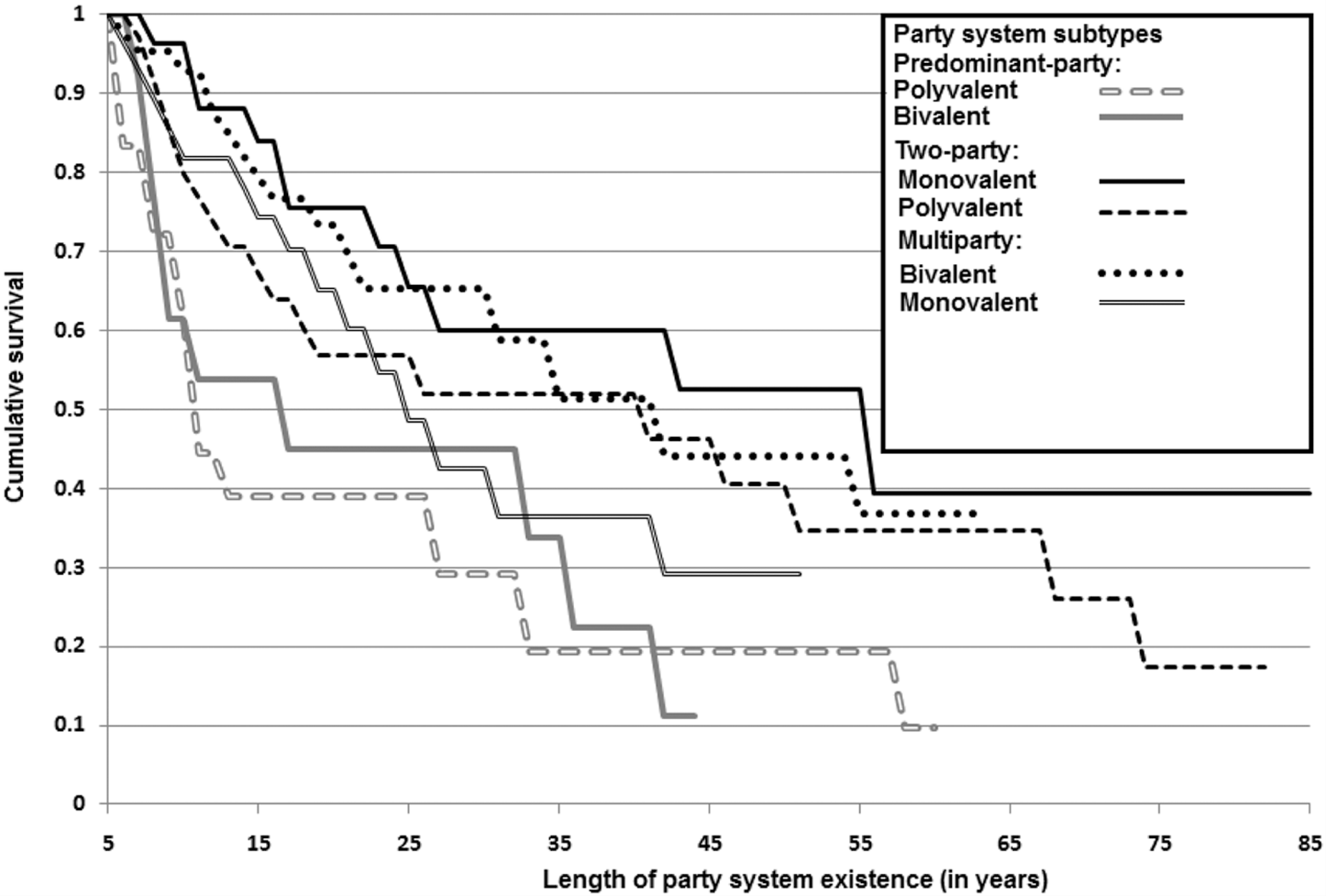
A plot of the Kaplan–Meier estimates of the survival functions for six party system subtypes.

Figure 9.

A possible alternative segmentation of the relative-size triangle.

Table 8.

Medians for survival time of different party system subtypes in the Kaplan–Meier estimator.

Party system subtype	Median, estimate	Standard error	95% confidence interval
Party system subtype	Median, estimate	Standard error	Lower bound	Upper bound
Polyvalent predominant-party	11	0.70	9.62	12.38
Bivalent predominant-party	17	6.79	3.70	30.30
Monovalent two-party	56	20.14	16.53	95.47
Polyvalent two-party	41	15.79	10.06	71.94
Bivalent multiparty	42	8.71	24.92	59.08
Monovalent multiparty	25	3.74	17.67	32.33

Conclusion

The purpose of this article was to produce a comprehensive classification of the world’s democratic party systems, and it is now delivered. While solving this task took effort, the immediate payoff, in terms of a better understanding of the global dynamics of party system development, is not negligible. The elementary quantitative judgment about the global spread and dynamics of the world’s democratic party systems is that predominant-party systems form the least-spread category; the two-party systems, found in approximately every third case, are more widespread; and multiparty systems are most common. To a certain extent, party systems vary depending on geographic region, with multipartism being best represented in Europe, and bipartism in the Americas, while predominant-party systems are most likely to be found in other regions of the world. The world of party systems is relatively stable over time, especially with regard to the share of two-party systems, but the third wave of democratization has brought about some new developments, including the relative decline of predominant-party systems and a great expansion of bivalent multiparty systems. The most durable party system is monovalent bipartism, but on this parameter bivalent multipartism is not very different, with the lowest longevity being consistently demonstrated by predominant-party systems. In general, however, the world of party systems remains diverse and sustains its diversity in the ongoing process of the global extension of democracy, which makes it imperative for political science to keep the tools of classification, such as the one used in this study, in a ready-to-use condition.

Footnotes

Acknowledgement

I am grateful to the anonymous referees of the journal for criticism and comments. All errors of fact and interpretation are entirely mine.

Notes

References

Blondel

(1968) Party systems and patterns of government in Western democracies. Canadian Journal of Political Science 1: 180–203.

Bogaards

(2004) Counting parties and identifying dominant party systems in Africa. European Journal of Political Research 43: 173–197.

Caramani

(2000) Elections in Western Europe Since 1815: Electoral Results by Constituencies. London and New York: Macmillan Reference.

Chhibber

Nooruddin

(2004) Do party systems count? The number of parties and government performance in the Indian states. Comparative Political Studies 37: 152–187.

Cook

(2001) European Political Facts of the Twentieth Century, 5th ed. New York: Palgrave.

Cox

Oakes

(1984) Analysis of Survival Data. London: Chapman and Hall.

Feger

(2001) Classification: Conceptions in the social sciences. In: Smelser

Baltes

(eds) International Encyclopedia of the Social and Behavioral Sciences, vol. 3: 1966–1973. Oxford: Elsevier.

Golosov

(2010) The effective number of parties: A new approach. Party Politics 16: 171–192.

Golosov

(2011) Party system classification: A methodological inquiry. Party Politics 17: 539--560 .

10.

Golosov

(2012) Towards a classification of the world’s democratic party systems, Step 1: Identifying the units. Party Politics, forthcoming; first published electronically on 31 May 2011 as doi: 10.1177/1354068811398059.

11.

Grofman

(1989) The comparative analysis of coalition formation and duration: Distinguishing between-country and within-country effects. British Journal of Political Science 19: 291–302.

12.

Grofman

Chiaramonte

D’Alimonte

Feld

(2004) Comparing and contrasting the uses of two graphical tools for displaying patterns of multiparty competition. Party Politics 10: 273–299.

13.

Gross

Sigelman

(1984) Comparing party systems: A multidimensional approach. Comparative Politics 16: 463–479.

14.

Huntington

(1991) The Third Wave: Democratization in the Late Twentieth Century. Norman, OK: University of Oklahoma Press.

15.

Laakso

Taagepera

(1979) ‘Effective’ number of parties: A measure with application to West Europe. Comparative Political Studies 12: 3–27.

16.

Landa

Ghiselin

(2005) The economics and bioeconomics of classification: Introduction. Journal of Bioeconomics 7: 215–220.

17.

Lijphart

(1994) Electoral Systems and Party Systems: A Study of Twenty-seven Democracies. Oxford: Oxford University Press.

18.

Mackie

Rose

(1991) International Almanac of Electoral History, 2nd ed. Washington, D.C.: Macmillan/CQ Press.

19.

Mainwaring

(1999) Rethinking Party Systems in the Third Wave of Democratization: The Case of Brazil. Stanford, CA: Stanford University Press.

20.

Mair

(2002) Comparing party systems. In: LeDuc

Niemi

Norris

(eds) Comparing Democracies 2: New Challenges in the Study of Elections and Voting. London: Sage, pp. 88–107.

21.

Nohlen

(ed.) (2005) Elections in the Americas: A Data Handbook, vols 1, 2. Oxford: Oxford University Press.

22.

Nohlen

Thibaut

Krennerich

(eds) (1999) Elections in Africa: A Data Handbook. Oxford: Oxford University Press.

23.

Nohlen

Grotz

Hartmann

(eds) (2001) Elections in Asia and the Pacific: A Data Handbook, vols 1, 2. Oxford: Oxford University Press.

24.

Ranney

Kendall

(1954) The American party systems. American Political Science Review 48: 477–485.

25.

Riker

(1982) The two-party system and Duverger’s Law: An essay on the history of political science. American Political Science Review 76: 753–766.

26.

Sanchez

(2009) Party non-systems: A conceptual innovation. Party Politics 15: 487–520.

27.

Sartori

(1976) Parties and Party Systems: A Framework for Analysis. Cambridge: Cambridge University Press.

28.

Shugart

Carey

(1992) Presidents and Assemblies: Constitutional Design and Electoral Dynamics. Cambridge: Cambridge University Press.

29.

Siaroff

(2000) Comparative European Party Systems: An Analysis of Parliamentary Elections Since 1945. New York and London: Taylor and Francis.

30.

Sikk

(2005) How unstable? Volatility and the genuinely new parties in Eastern Europe. European Journal of Political Research 44: 391–412.

31.

Von Bertalanffy

(1968) General System Theory: Foundations, Development, Applications. New York: George Braziller.

32.

Ware

(1996) Political Parties and Party Systems. Oxford: Oxford University Press.

33.

Wolinetz

(2006) Party systems and party system types. In: Katz

Crotty

(eds) Handbook of Party Politics. London: Sage, pp. 51–62.