Forecasting tourism demand using search query data: A hybrid modelling approach

Abstract

Search query data have recently been used to forecast tourism demand. Linear models, particularly autoregressive integrated moving average with exogenous variable models, are often used to assess the predictive power of search query data. However, they are limited by their inability to model non-linearity due to their pre-assumed linear forms. Artificial neural network models could be used to model non-linearity, but mixed results indicate that their application is not appropriate in all situations. Therefore, this study proposes a new hybrid model that combines the linear and non-linear features of component models. The model outperforms other models when forecasting tourist arrivals in Hong Kong from mainland China, thus demonstrating the advantage of adopting hybrid models in forecasting tourism demand with search query data.

Keywords

artificial neural network hybrid specification non-linear model search query data tourism forecasting

Introduction

The need for accurate forecasts of tourism demand has long been recognized by tourism researchers, policymakers and practitioners. Policymakers need accurate forecasts to allocate resources for the construction of tourism infrastructure, such as hospitality facilities and public transportation. Due to the perishable nature of tourism products, it is impossible to stockpile unsold airline seats and hotel rooms. Thus, accurate forecasts of business demand are crucial for practitioners to make better business decisions, such as staffing decisions, and to formulate pricing strategies.

Traditional tourism demand forecasting involves gathering historical data to construct various models, including time series, econometric and artificial intelligence models (Song and Li, 2008). However, the ubiquitous use of the Internet means that traces of these online activities are now being recorded on a massive scale. These digital footprints constitute big data that reflect users’ intentions, preferences and interests and thus have the potential to improve modelling and forecasting in a wide array of areas. Researchers have adopted different types of big data, such as search query and social media data, to forecast activities such as claims for unemployment (Choi and Varian, 2012), influenza epidemics (Ginsberg et al., 2009) and box-office revenue trends (Arias et al., 2013).

Studies have also investigated the effectiveness of big data in forecasting tourism demand. Search queries are among the most commonly used types of data (Choi and Varian, 2012; Li et al., 2017; Pan et al., 2012; Yang et al., 2015). Before travelling (Fesenmaier et al., 2010), many tourists search online for relevant information about accommodation, attractions and activities (Pan et al., 2006). These search query volumes can be retrieved from search engines to provide early indicators of future trips and, thus, to predict future tourism demand.

Previous studies that have attempted to forecast tourism demand from search query data have used traditional statistical models, particularly the autoregressive integrated moving average with exogenous variable (ARIMAX) model (Choi and Varian, 2012; Li et al., 2017; Yang et al., 2015). Although the forecasting performance of these models is better than that of the benchmark models due to their inclusion of search query data, they still have limitations due to their pre-assumed linear forms.

In contrast, artificial neural network (ANN) models have the advantage of being able to model non-linearity and have been used for tourism demand forecasting (Kon and Turner, 2005; Law and Au, 1999; Palmer et al., 2006). ANN models perform better than traditional linear models in forecasting non-linear time-series data (Zhang et al., 2001). A composite index must often be constructed due to the large amount of information that big data provide. This can create a complicated relationship between the index and the variable we want to predict, which cannot be fully explained by linear models (Arias et al., 2013). A non-linear autoregressive with exogenous variable (NARX) model can be used to capture the non-linearity.

Both autoregressive integrated moving average (ARIMA) and ANN models have proved to be successful in their own linear and non-linear domains, neither type is suitable for all situations. It is widely accepted in the forecasting literature that no single model is superior in all situations. Real-life time-series data are often complex and may involve both linear and non-linear patterns that cannot be adequately modelled by either ARIMA or ANN. Combining the two can alleviate the problem (Zhang, 2003). Due to the combination of the linear and non-linear features, hybrid models have been proved to outperform both of the individual component models in univariate time-series forecasting (Khashei and Bijari, 2011; Tseng et al., 2002; Zhang, 2003). Hybrid models with the linear and non-linear components are likely to be better at modelling the complex relationship between tourism demand and a composite search index.

Although several studies have found search query data to be useful in forecasting tourism demand, only linear models were used (Li et al., 2017; Yang et al., 2015). No study has explored the possible non-linear relationship between search query data and tourism demand. This study fills this gap by comparing the results of the ARIMA and non-linear autoregressive (NAR) neural network models with those of the ARIMAX and NARX models, respectively. An extension of a hybrid model that includes an explanatory variable is proposed. The results of the ARIMAX model in the first stage are then used as inputs for the NARX model in the second stage. This novel hybrid model contributes to the modelling literature, which is dominated by linear models, because it is capable of capturing both the linearity and non-linearity common to real-life data.

The remainder of this article is organized as follows. The second section presents the relevant literature, followed by the introduction of data and preliminary tests in the third section. Then, in the fourth section, the model construction and results are provided and finally, the conclusions are drawn in the fifth section.

Literature review

In this section, we begin by reviewing the literature on tourism demand forecasting. We then review the application of forecasting using search query data and consider ANN and hybrid model forecasting studies. Research gaps are identified at the end of the section.

Tourism demand forecasting

Song and Li (2008) provided a detailed review of tourism demand modelling and forecasting. There are three main types of modelling techniques: time series, econometric and artificial intelligence models.

Time-series models that generate forecasts based on past values are widely used in tourism demand forecasting. This makes data collection less expensive, as only one variable is needed to build the model. The most commonly used time-series model is the ARIMA model proposed by Box and Jenkins (1970). Various extensions of the ARIMA model have also been used. When seasonal data are used, the seasonal ARIMA model can be used to capture the seasonality of tourism demand. Goh and Law (2002) introduced the ARIMA model with intervention to forecast 10 arrival series for Hong Kong and found that the model outperformed other time-series models. Simpler models such as naive and exponential smoothing models are also often used, but they are more frequently used as benchmark models.

Econometric models can be used when influencing factors that might have causal relationships with tourism demand need to be included. Traditional regression models, such as the ordinary least squares model, suffer from the spurious regression problem (Song and Li, 2008). Therefore, more advanced econometric models have been used, such as the autoregressive distributed lag model (Song et al., 2003), error correction model (Kulendran and Wilson, 2000), vector autoregressive model (Song and Witt, 2006), time-varying parameter model (Song and Wong, 2003) and almost ideal demand system model. Although some studies have found that econometric models outperform time-series models in forecasting tourism demand (Song et al., 2003), others have found that time-series models forecast more accurately (Athanasopoulos et al., 2011; Witt and Witt, 1995). Song and Li (2008) concluded that no single model can outperform all other models in all situations.

Various artificial intelligence techniques have been used to forecast tourism demand, such as fuzzy logic, genetic algorithms and, most notably, the ANN model. Unlike traditional time-series and econometric models, the ANN model can model the non-linearity in the data. Law (2000) used a back-propagation ANN model and found that it outperformed regression and time-series models in forecasting Taiwanese visitors to Hong Kong. Cho (2003) compared three approaches to forecast tourist arrivals in Hong Kong and found that the ANN model performed better than the ARIMA and exponential smoothing models. Kon and Turner (2005) compared the ANN model with the basic structural, naive and Holt-Winters models in forecasting arrivals in Singapore and found that a correctly specified ANN model could outperform the other models. Although most studies have asserted that ANN models can forecast tourism demand accurately, some have suggested that they are outperformed by simpler time-series models. Claveria and Torra (2014) demonstrated that a simple ARIMA model could outperform an ANN model in forecasting tourism demand in Catalonia.

Forecasting with search query data

The Internet has made it incredibly easy to find information, and using search engines is a part of people’s daily lives (Sparrow et al., 2011). Online search behaviour is related to users’ consumption preferences and decision-making processes (Du et al., 2014; Ghose et al., 2014). In recent years, using search query data for forecasting has become commonplace in numerous research areas.

One of the first efforts was made by Ginsberg et al. (2009) who demonstrated the feasibility of detecting influenza epidemics using a large number of Google search queries. Vosen and Schmidt (2011) forecasted private consumption based on factors extracted from Google search queries. The Google indicators outperformed the two most common survey-based indicators in almost all in- and out-sample forecasting experiments. Bordino et al. (2012) showed that daily volumes of search queries related to stocks traded on the NASDAQ-100 were correlated with the trading volumes of the same stocks and, in many cases, predicted trading peaks by one day or more. Other studies have used search query data to forecast unemployment rates (Askitas and Zimmermann, 2009), automotive sales (Du and Kamakura, 2012) and consumer confidence (Choi and Varian, 2012).

Studies using search query data to forecast tourism demand have emerged in the last few years. Choi and Varian (2012) used the average Google Trends index for vacation destinations in Hong Kong for the first 2 weeks of every month by country of origin to predict the tourism demand in that month. Pan et al. (2012) used the search volumes of five related queries for a specific tourist city to predict demand for hotel rooms. They compared different models and found that autoregression with an exogenous variable model generated better forecasting performance than other models. They also pointed out that their study included only a limited number of search queries and that a larger number of queries could be used to increase forecasting accuracy. Yang et al. (2015) used a large number of search queries from two search engines, Google and Baidu, to forecast tourism demand for a popular tourist city in China and proposed a method for selecting relevant search queries. They found that although search query data from both search engines improved forecasting accuracy compared with the baseline model, the Baidu Index data appeared to outperform the Google Trends data in forecasting tourism demand. Bangwayo-Skeete and Skeete (2015) found that the forecasting performance of tourist arrivals in five popular tourist destinations in the Caribbean was superior to that of the alternative models when the mixed-data frequency approach that incorporates the Google Trends information was used. Rivera (2016) retrieved Google Trends data in 11 different occasions and found that the dynamic linear model provided better forecasts than the simpler models. Önder and Gunter (2016) used Google Trends data to forecast tourism demand in Vienna. Their results confirmed that the models’ forecasting performance was improved when Google Trends data are included across the source markets for both seasonal and seasonally adjusted data. Li et al. (2017) used search queries from Baidu to predict the tourism demand for Beijing and found that forecasting performance was improved by the inclusion of a composite search index.

Forecasting using ANN and hybrid models

The most basic computing units in ANN models are nodes (or neurons). Although numerous types of ANN have been proposed, the most popular and widely adopted is the multilayer feedforward network model, which usually consists of input, hidden and output layers. Hornik et al. (1989) rigorously established that one hidden layer was enough for multilayer feedforward networks to be universal approximators.

Scholars have adopted ANN models to forecast time-series data. Hill et al. (1996) compared the time-series forecasting performance of an ANN model with six statistical time-series techniques generated in a major forecasting competition. They found that the ANN performed significantly better than traditional methods across monthly and quarterly time series.

Refenes et al. (1994) showed that an ANN model outperformed classical statistical techniques in forecasting stock performance and noted that the traditional techniques had limitations in forecasting applications with non-linearity. Zhang et al. (2001) conducted an experimental evaluation of ANNs for non-linear time-series forecasting and showed that neural networks are valuable tools for forecasting non-linear time-series data, whereas traditional linear methods are unsuitable for this task.

Choosing an appropriate structure for an ANN model is important, yet there is no systematic procedure to guide the model-building process. For example, an appropriate number of input and hidden nodes must be specified: Specifying too many can make the ANN model too specific and may cause an overfitting problem, thus deteriorating the forecasting performance. In practice, appropriate experimental parameters are often chosen through trial and error. There are other issues in building ANN models, such as the choice of activation function and training algorithm (Zhang et al., 1998). Faraway and Chatfield (1998) found that ANN models outperformed the Box–Jenkins model in forecasting airline time-series data only when the former were built with appropriate structures.

Although ANN models perform better than traditional linear models in some studies, other studies have reported inconsistent results. Foster et al. (1992) found that ANN models presented significantly less accurate forecasts than traditional linear regression. Denton (1995) found little difference between linear regression and neural network models in causal forecasting under ideal conditions. ANN models may perform worse than linear statistical models in some cases, because the underlying data are linear without much disturbance (Zhang et al., 1998). The mixed results from ANN models suggest that it is inappropriate to apply them blindly in all situations.

As it is difficult to know the underlying pattern of real-life data and whether it is rarely purely linear or non-linear, the use of hybrid models that have both linear and non-linear modelling capabilities tends to be a good strategy. For example, Zhang (2003) suggested a hybrid method that combined the features of the ARIMA and ANN models to take advantage of their unique linear and non-linear modelling strengths. Their experimental results indicated that the hybrid model improved the forecasting accuracy compared with the individual models. Tseng et al. (2002) proposed a hybrid forecasting model that combined seasonal ARIMA and neural network backpropagation models. The hybrid model outperformed seasonal ARIMA and two neural network models with differenced and deseasonalized data in forecasting two-seasonal time-series data. Khashei and Bijari (2011) proposed a novel hybridization of the ANN and ARIMA models. Their model preserved and magnified the linear features of the ARIMA model, and the ANN model was used to capture the underlying data-generating process. Their empirical results indicated that the proposed model produced more accurate forecasts than traditional hybrid models and either of the component models used separately. Aslanargun et al. (2007) used various combinations of ARIMA and ANN models to forecast tourist arrivals in Turkey and found that models with non-linear components exhibited better performance.

Considering the potentially complex relationship between tourism demand and the composite search index, univariate time-series hybrid models could be extended to include the composite search index as an exogenous variable. This study proposes a new hybrid ARIMAX/NARX model. The linear models used in previous studies were incapable of capturing the possible non-linear relationship between search data and tourism demand. This study fills this gap using the proposed hybrid model to capture both linearity and non-linearity.

Preliminary data analysis

Tourist arrivals data

Tourist arrivals in Hong Kong from mainland China are used as the tourism demand data for the empirical study. According to A Statistical Review of Hong Kong Tourism 2015 by the Hong Kong Tourism Board, there were 45.8 million arrivals from mainland China in 2015, accounting for 77% of Hong Kong’s total arrivals. The Hong Kong Tourism Board publishes monthly tourist arrivals data with a lag of about 1 month, and the data can be collected from the official website. As the search query data used in this study are only available from 2011, we collect the tourist arrivals data from January 2011 to September 2016. The tourist arrival data are log transformed, following conventional practice.

Composite search index construction

As we are interested in tourists from mainland China visiting Hong Kong, we use search engines in the Chinese market. Baidu has the largest market share in China, and an earlier study confirmed that Baidu search data could better predict Chinese tourists’ travel patterns (Yang et al., 2015). Thus, we use Baidu as the search engine to collect search query data. The daily volumes of search queries are available from 2011 provided by Baidu Index.

The most commonly used method for selecting search query data is based on the researcher’s intuition and knowledge (Brynjolfsson et al., 2014). This method is also adopted in this study. Some studies have selected several specific search queries and directly used the volumes of these search queries to predict tourism demand (Pan et al., 2012). This method has the potential problem of omitting important information by excluding relevant search queries. Recent studies have suggested a systematic procedure for selecting tourism-related search queries (Li et al., 2017; Yang et al., 2015). First, some aspects of trip planning are specified. Tourists generally make their travel decisions based on the economic factors such as their income levels, the costs of travel and their destination preferences (Jeng and Fesenmaier, 2002). However, after choosing the destination, tourists normally search for the details online about different aspects of the destination that they chose. Following the earlier studies such as Yang et al (2015) and Li et al. (2017), six aspects are chosen in this study: dining, shopping, traffic, tours, attractions and lodgings. Second, several initial search queries are specified for each aspect. Third, these search queries are entered into the Baidu Index; highly correlated search queries can be collected from a demand map interface provided by the Baidu Index. This step is iterated, after which the number of search queries converges to 126. Lastly, as the Baidu Index does not provide the volumes of search queries below a certain threshold, the availability of each search query is manually checked in the Baidu Index, and only those that are available are saved as final search queries. Finally, there are 64 search queries and their volumes are available on a daily basis starting from 2011. The daily tourist arrivals data are aggregated into monthly data spanning January 2011 to September 2016.

The translated search query terms and their correlations with the arrivals data are given in Table 1.

Table 1.

Correlation between search query and arrivals data.

Search query name	Correlation	Search query name	Correlation
Dining		Tour
Hong Kong food	0.806	Hong Kong travel guidance	0.492
Hong Kong snack	0.786	Hong Kong self-guided tour guidance	0.243
Hong Kong food guidance	−0.047	Hong Kong travel guide	0.589
Hong Kong food recommendation	0.724	Hong Kong tourism guidance	0.462
Hong Kong specialty	0.839	Hong Kong tourism guidance self-guided tour	0.723
Which are Hong Kong specialties	0.799	Hong Kong weather	0.261
Hong Kong specialty food	0.739	Hong Kong weather forecasting	0.674
		Hong Kong one-day trip	0.688
Shopping		Hong Kong one-day trip guidance	0.715
Hong Kong shopping	0.577
Hong Kong shopping list	0.701	Attraction
Hong Kong shopping guidance	0.701	Hong Kong tourist attractions	0.282
Hong Kong Ladies Market	0.363	Hong Kong tourist attractions introduction	−0.536
What is worth buying in Hong Kong	0.775	Hong Kong Ocean Park	0.688
Hong Kong shopping guide	−0.190	Hong Kong Times Square	0.793
Hong Kong shopping map	0.303	Hong Kong Mong Kok	0.481
Hong Kong travel shopping guide	0.263	Hong Kong Causeway Bay	0.857
Go to Hong Kong shopping guidance	0.780	Hong Kong Avenue of Stars	0.670
Hong Kong Mong Kok shopping guidance	0.840	Hong Kong Victoria Harbour	0.791
		Hong Kong attractions	0.832
Traffic		Madame Tussauds Hong Kong	0.728
Hong Kong map	0.180	Hong Kong Ocean Park guidance	0.595
Hong Kong subway	0.929	Hong Kong Ocean Park ticket	0.692
Hong Kong subway circuit map	0.857	Hong Kong Disneyland	0.728
Hong Kong whole map HD	0.807	Hong Kong Disneyland resort	0.733
Hong Kong subway map	0.489	Hong Kong Ocean Park ticket price	0.103
Hong Kong travel map	−0.200	Hong Kong Disneyland ticket price	0.480
Hong Kong subway price	0.880	Hong Kong Disneyland guidance	0.783
Hong Kong subway schedule	0.771
Hong Kong airport	0.816	Lodging
Hong Kong airport express	0.880	Hong Kong hotels	0.075
Hong Kong airport duty-free shop	0.358	Peninsula Hotel Hong Kong	0.601
Octopus card	0.878	Hong Kong hotel booking	0.296
		Hong Kong accommodation	0.708
		Four Seasons Hotel Hong Kong	0.568
		Hong Kong hotels recommendation	0.853
		Hong Kong hotel booking website	−0.525
		Hong Kong hotel group booking	0.366
		L’hotel Nina Et Convention Centre	0.549

Note: HD: high definition.

After obtaining the volumes of the relevant search queries, it is important to decide how to extract information from this large amount of data. It is not viable to add the volumes of so many search queries directly into the model because doing so would create many degrees of freedom and cause an overfitting problem. Principal component analysis (PCA) is a dimension reduction tool that uses orthogonal transformation to produce linearly uncorrelated principal components (PCs), which are linear combinations of original data. Most variations in the original data can be preserved by choosing the first few PCs. PCA can be used to construct a composite index from a large number of search queries, and it has been applied in other studies (Li et al., 2015; Li et al., 2017). Such a composite index also has the advantage of being less volatile than an individual search query. In practice, normalization, which is also adopted in this study, is often achieved by subtracting the mean and dividing by the standard deviation for each search query before applying PCA. Applying this procedure can better reflect the variations of search queries with relatively low volumes. The variance contribution rates of the PCs are plotted in Figure 1.

Figure 1.

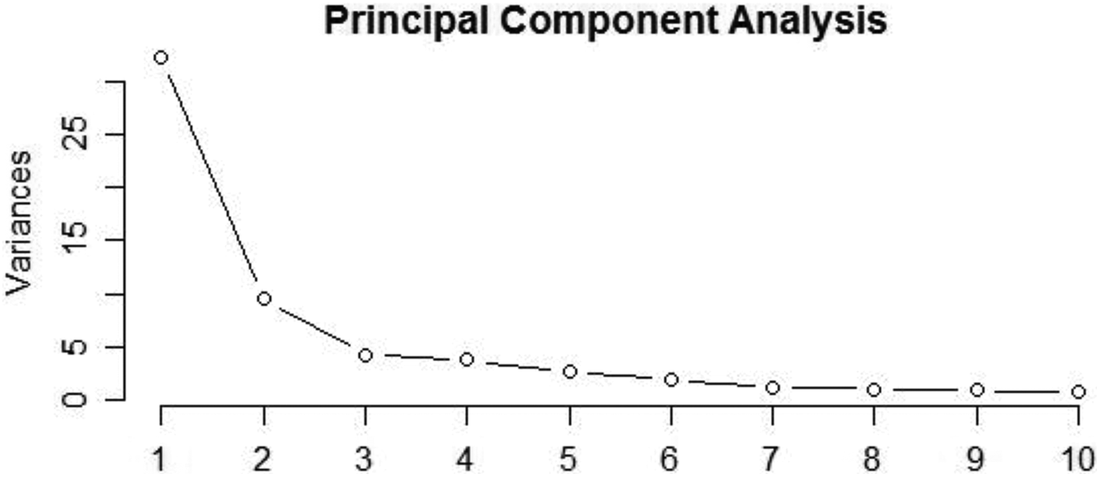
Variance contribution rates.

The first PC explains more than 30% of the variance, and there is a large drop in the contribution rate from the second PC. The scree plot criterion suggests to choose the factors until a break in the graph. Since there is a clear break after the first PC, only the first PC is retained as the composite search index in this study. This study does not intend to explain the majority of the variance of the search queries as our focus is to extract information from the search queries to improve the accuracy of tourism demand forecasts.

The top 10 queries that have the largest weights in the PC are listed in Table 2.

Table 2.

Queries with top 10 biggest weights for PC.

Query	Weights
Octopus card	0.1699
Hong Kong airport express	0.1685
Hong Kong subway	0.1622
Hong Kong attractions	0.1622
Hong Kong hotels recommendation	0.1618
Hong Kong subway circuit map	0.1617
Hong Kong Mong Kok shopping guidance	0.1601
Go to Hong Kong shopping guidance	0.1598
Hong Kong airport	0.1588
Hong Kong subway schedule	0.1584

Note: PC: principal component.

The top 3 queries, and indeed 6 of the top 10, are related to traffic, suggesting that tourists from mainland China travelling to Hong Kong most commonly search for traffic information. Figure 2 shows the relationship between the PC and arrivals data.

Figure 2.

Relationship between the first PC and arrivals data. PC: principal component.

A strong concordance can be seen between the arrivals data and PC. However, the underlying relationship requires further investigation using more tests and modelling.

Preliminary tests

Some statistical tests can be conducted before the modelling to assess the relationship between the arrivals data and PC. There are several methods for testing linearity, and some neural network-based tests have been shown to work well in many fields (Lee et al., 1993; White, 1989). Teräsvirta et al. (1993) demonstrated that the Teräsvirta neural network test appeared superior to the other tests overall. It is implemented by testing the null hypothesis of linearity between the arrivals data and the PC. The results are given in Table 3.

Table 3.

Linearity test.

Teräsvirta neural network test
X ²	9.8274
Degrees of freedom	2
p-Value	0.007345

The small p-value of the Teräsvirta neural network test suggests that the null hypothesis of linearity between the arrivals data and PC should be rejected. This indicates that traditional linear models such as the ARIMAX may not be able to adequately model the relationship between the arrivals data and the PC.

Granger causality tests (Granger, 1969) are often conducted to assess the causal relationship between variables. The basic idea is that if a random variable X Granger causes another variable Y, then the past values of X should contain information that helps to predict Y in addition to the information contained in the past values of Y. Traditional parametric tests involve building a vector autoregressive model to test the null hypothesis that all coefficients of lagged X are zero in a linear regression model where Y is dependent on the past values of both X and Y (Toda and Yamamoto, 1995). Rejection of the null hypothesis suggests that X Granger causes Y. However, the limitation of the parametric Granger causality test is that it assumes a linear relationship between the variables. As the Teräsvirta neural network test indicated non-linearity between the arrivals data and PC, it may not be appropriate to test Granger causality in a linear form. Some non-parametric tests that can test for non-linear Granger causality have been suggested. We use a non-parametric Granger causality test proposed by Diks and Panchenko (2006), because it overcomes some of the problems of earlier tests and proves to work well in applications. According to the results in Table 4, the null hypothesis that the PC does not Granger cause tourist arrivals is rejected at the 5% significance level. This suggests that the PC Granger causes tourist arrivals and, thus, is predictive of tourist arrivals.

Table 4.

Non-parametric Granger causality test.

Null hypothesis	PC does not Granger cause arrivals data	Arrivals data did not Granger cause PC
T-statistics	2.21	0.289
p-Value	0.01356	0.38629

Note: PC: principal component.

Competing models

ARIMA and ARIMAX

We construct the ARIMA and ARIMAX models with the PC as an exogenous variable. In the following, TA denotes the log-transformed tourist arrivals data. The data from January 2011 to September 2015 are used to train the models, and the data from the 12 months from October 2015 to September 2016 are used for forecasting.

A seasonal ARIMA(p, d, q)(P, D, Q) _m model can be written as follows

Φ (B^{m}) φ (B) {(1 - B^{m})}^{D} {(1 - B)}^{d} y_{t} = c + Θ (B^{m}) θ (B) ∊_{t}

where

B

is the backshift operator,

Φ (x)

and

Θ (x)

are polynomials of orders P and Q, respectively,

φ (x)

and

θ (x)

are polynomials of orders p and q, respectively and

∊_{t}

is a white noise process with a mean of zero and a variance of σ ². ARIMA models are often estimated following the Box–Jenkins approach. Hyndman and Khandakar (2008) proposed an automatic order selection process for the ARIMA model. First, the order of seasonal differencing D is chosen based on the OCSB test (Osborn et al., 1988). Second, the order of non-seasonal differencing d is chosen using the KPSS unit-root test (Kwiatkowski et al., 1992). Third, a stepwise procedure is used to traverse the model space to choose the order of autoregressive and moving average terms, p, q, P and Q. The model with the lowest Akaike information criterion is then chosen. This automatic process is applied to TA.

The ARIMAX model is constructed in a similar way to the ARIMA model, except that a linear regression of TA on the lagged PC is conducted first and the automatic order selection process is used after the effect of the lagged PC is eliminated. The PC has strong positive autocorrelations that die out very slowly, as can be seen in Figure 3. The horizontal blue dashed lines are placed at zero plus and minus two approximate standard errors of the sample autocorrelations. Most sample autocorrelations are way above the positive blue dashed line, suggesting a large correlation for the PC with different lags. To avoid multicollinearity caused by including multiple lags of the PC at the first linear regression step, only the PC with a lag equal to one is included in the ARIMAX model.

Figure 3.

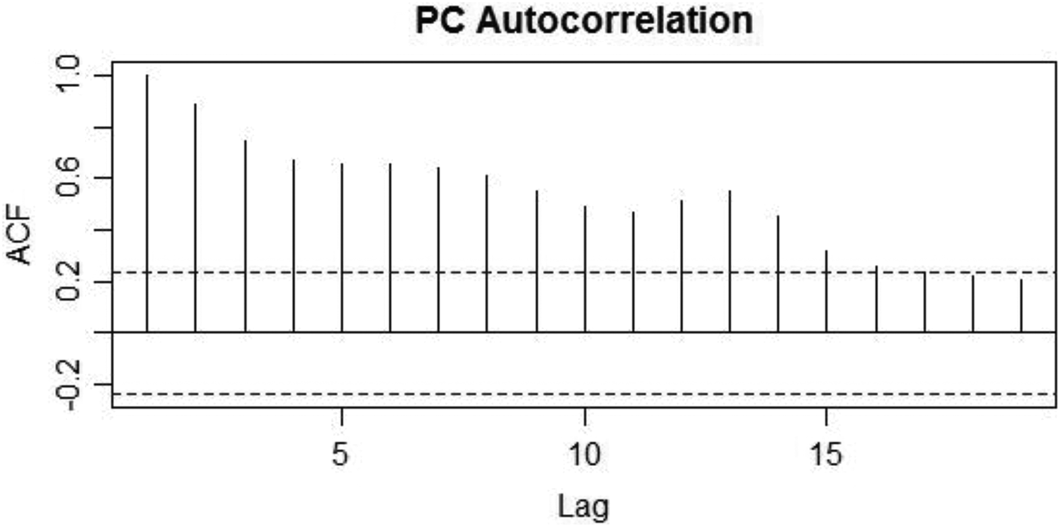
Sample autocorrelation of PC. ACF: Autocorrelation Function. PC: principal component.

The resulting models are ARIMA(0,1,2)(1,0,0)₁₂ and ARIMAX(0,1,1)(0,1,1)₁₂. The details are given in Table 5.

Table 5.

Results of the ARIMA and ARIMAX models.

ARIMA		ARIMAX
Non-seasonal differencing	Yes	Non-seasonal differencing	Yes
Seasonal differencing	No	Seasonal differencing	Yes
MA(1)	−0.8666***	MA(1)	−0.7439***
MA(2)	0.2923**	SMA(1)	−0.3254*
SAR(1)	0.8867***	PC _t _{− 1}	0.0246***
Residual variance	0.004999	Residual variance	0.004346
AIC	−113.64	AIC	−105.49
BIC	−105.53	BIC	−98.44
p-Value of Ljung–Box	0.7741	p-Value of Ljung–Box	0.2369

Note: ARIMA: autoregressive integrated moving average; ARIMAX: autoregressive integrated moving average with exogenous variable; SAR: seasonal autoregressive term; SMA: seasonal moving average; PC: principal component; AIC: Akaike information criterion; MA: moving average; BIC: Bayesian Information Criterion.

***Estimates are significant at the 1% level.

**Estimates are significant at the 5% level.

*Estimates are significant at the 10% level.

SAR denotes the seasonal autoregressive term, and SMA denotes the seasonal moving average term. The fitted ARIMA and ARIMAX models can be expressed as follows

ARIMA: (1 - 0.8867 B^{12}) (1 - B) {TA}_{t} = (1 - 0.8666 B + 0.2923 B^{2}) ∊_{t}

ARIMAX : {\begin{matrix} TA = 0.0246 {PC}_{t - 1} + u_{t} \\ (1 - B^{12}) (1 - B) u_{t} = (1 - 0.7439 B) (1 - 0.3254 B^{12}) ∊_{t} \end{matrix}

ARIMAX has seasonal and non-seasonal differencing, while ARIMA has non-seasonal differencing and SAR. PC _t _{− 1} is significant at the 1% level and indicates that the composite search index is predictive of tourist arrivals. The Ljung–Box test is conducted, and the p-value suggests that there is no autocorrelation in the residuals for the ARIMA and ARIMAX models.

NAR and NARX

The appropriate construction of an ANN model is important, but there is no systematic approach that guides this process. For example, there is no standard rule that determines the number of layers and number of nodes in each hidden layer, although using one hidden layer is sufficient for most practical problems (Hornik et al., 1989; Zhang et al., 1998). Thus, we use a single hidden layer, and the number of nodes in the hidden layer and the number of delays are determined experimentally.

To obtain good predictions with ANN models, it is important to prevent overfitting to preserve their generalizing ability. Several methods can be used to solve the overfitting problem. One method is to create a validation data set that imposes early stopping when the performance stops improving. Another method is to add a regularization term into the model, but the regularization parameters must be chosen beforehand. An automated training algorithm based on the Bayesian framework can be used to address this problem (MacKay, 1992). The regularization parameters can be determined based on the variance of weights in the ANN model, which are assumed to be random variables. Creating a validation data set reduces the number of observations that can be used in the training process. Considering the relatively short length of the data set in this study, the Bayesian regularization is adopted to prevent overfitting.

The form of the data should also be considered before they are applied to neural network training. Although there is no consensus as to whether the data should be deseasonalized before use, most studies have found that ANN models give better results in forecasting time-series data if they are deseasonalized (Nelson et al., 1999; Zhang and Qi, 2005). In the context of tourism demand forecasting, Palmer et al. (2006) found that using preprocessing by seasonally differencing data produced better forecasts of tourism expenditure in the Balearic Islands, perhaps due to the large number of hidden nodes required to adequately model time-series data based on trend and seasonality. Considering that the amount of data available in the tourism field is usually very limited, which is also the case in this study, an ANN model with too many parameters is likely to cause overfitting. The most effective solution is to eliminate the deterministic components first and concentrate on learning the nondeterministic components of the data. This approach is implemented in this study using seasonally differenced data, denoted as DTA and DPC for seasonally differenced TA and PC, respectively.

Although it is possible to use different activation functions for different nodes in the same or different layers, almost all ANN models use the same activation for the same layer (Zhang et al., 1998). The following hyperbolic tangent function is often used as an activation function in forecasting problems

f (x) = (exp (x) - exp (- x)) / (exp (x) + exp (- x))

This non-linear function can be used to introduce non-linearity into the model. In this study, it is used as the activation function for the hidden layer. The linear activation function for output nodes is often used for forecasting problems that involve continuous target values (Rumelhart et al., 1995). As we are forecasting time-series data in this study, we adopt it as the activation function for the output layer. Finally, it is recommended that the range of variables should be limited in the work interval of the activation functions used in the hidden and output layers to avoid computational problems and facilitate network learning (Srinivasan et al., 1994). As the hyperbolic tangent function has an output interval of [−1, 1], the data are transformed to this interval using linear transformation.

Two further parameters need to be chosen for the NAR model: The number of hidden nodes and the lags for DTA that should be used as inputs. The mean squared error (MSE) is used as the criterion for choosing these two parameters experimentally. The model with fewer parameters is chosen when two models give the same MSE, as parsimonious models often have better generalization capability and better forecasting performance. The results of different combinations of hidden nodes and lags are listed in Table 6.

Table 6.

MSE results of the NAR model.

Hidden nodes	DTA lags
Hidden nodes	1	2	3
1	0.0066	0.0061	0.0046
2	0.0062	0.0047	0.0046
3	0.0062	0.0061	0.0046

Note: DTA: seasonally differenced tourist arrivals; MSE: mean squared error; NAR: non-linear autoregressive.

The model with one hidden node and three lags of DTA is the most parsimonious among models with the smallest MSE of 0.0046. Models with more lags of DTA are also explored, but the MSE does not decrease further. Thus, an NAR model with one hidden node and three lags of DTA is chosen for forecasting.

The same model-building procedure is applied to the NARX model, with the exception of choosing the number of lags for DPC. The results with one and two lags of DPC are given in Table 7.

Table 7.

MSE results of the NARX model.

One lag of DPC				Two lags of DPC
Hidden nodes	DTA lags			Hidden nodes	DTA lags
Hidden nodes	1	2	3	Hidden nodes	1	2	3
1	0.0051	0.0046	0.0034	1	0.0052	0.0044	0.0034
2	0.0051	0.0046	0.0034	2	0.0052	0.0044	0.0034
3	0.0051	0.0046	0.0034	3	0.0052	0.0044	0.0034

Note: DPC: seasonally differenced principal component; MSE: mean squared error; NARX: non-linear autoregressive with exogenous variable.

Models with one and two lags of DPC give similar MSE results. Models with more lags for DPC and DTA are also fitted, but they do not give better MSE results. Compared with the NAR model, the NARX model has a smaller MSE, indicating its better fit with the inclusion of lagged DPC. Based on the parsimonious rule, an NARX model with three DTA lags, one DPC lag and one hidden node is chosen for forecasting.

Hybrid model

The hybrid model is constructed by combining the ARIMAX and NARX models. Linear modelling is accomplished by constructing an ARIMAX model, as described earlier, and the results are saved for the non-linear modelling stage. The residuals and one-step-ahead predictions from the ARIMAX model are used as inputs to the NARX model. The one-step-ahead prediction from the ARIMAX model for time t, denoted by ${\hat{T A}}_{t}$ , is available at time t − 1. Lagged PC and lagged TA are also used as inputs for the NARX model. TA is used as the output. The same construction procedure is applied to choose the appropriate lags for the inputs and the number of hidden nodes. The final hybrid model has two hidden nodes, and the inputs at time t can be summarized as follows:

one-step-ahead prediction from ARIMAX, ${\hat{T A}}_{t}$ ;

residual from ARIMAX with lag 1, $e_{t - 1}$ ;

PC with lag 1, ${PC}_{t - 1}$ ; and

TA with lag 1, ${TA}_{t - 1}$ .

Forecast comparison

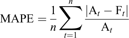
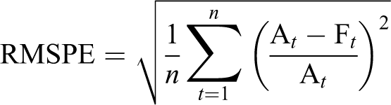
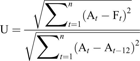
To examine the predictive power of the search query data and whether the hybrid model can outperform other models, we compare the forecasting results for all five models from October 2015 to September 2016. Performance is assessed using five measures: the mean absolute deviation (MAD), MSE, mean absolute percentage error (MAPE), root mean square percentage error (RMSPE) and Theil’s U statistic. The MAD measures the average accuracy by weighting the absolute deviations equally. The MSE takes the average squared errors, so that large errors have bigger impacts. The MAPE is similar to the MAD, but uses the percentage errors. The RMSPE uses squared percentage errors and takes the square root of the mean. Theil’s U is used to evaluate the forecasting performance of the model against the seasonal naive model. If Theil’s U is less than one, it indicates that the forecasting technique performs better than the seasonal naïve method. Each of these measures is defined as follows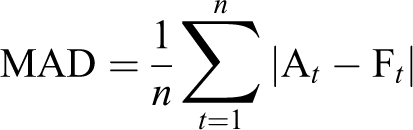

MAD = \frac{1}{n} \sum_{t = 1}^{n} | A_{t} - F_{t} |

MSE = \frac{1}{n} \sum_{t = 1}^{n} {(A_{t} - F_{t})}^{2}

MAPE = \frac{1}{n} \sum_{t = 1}^{n} \frac{| A_{t} - F_{t} |}{A_{t}}

RMSPE = \sqrt{\frac{1}{n} \sum_{t = 1}^{n} {(\frac{A_{t} - F_{t}}{A_{t}})}^{2}}

U = \frac{\sqrt{\sum_{t = 1}^{n} {(A_{t} - F_{t})}^{2}}}{\sqrt{\sum_{t = 1}^{n} {(A_{t} - A_{t - 12})}^{2}}}

where

A_{t}

denotes the actual value,

F_{t}

denotes the forecast value in forecasting period t and n is the length of the forecasting period, which is equal to 12. The forecasting performance results for all of the models are given in Table 8.

Table 8.

Forecasting result with last 12 months as testing set.

Measure	ARIMA	ARIMAX	NAR	NARX	Hybrid
MAD	253,402 (5)	165,975 (2)	228,649 (4)	213,920 (3)	125,607 (1)
MSE	8.72 × 10¹⁰ (3)	4.23 × 10¹⁰ (2)	9.91 × 10¹⁰ (5)	8.77 × 10¹⁰ (4)	3.03 × 10¹⁰ (1)
MAPE (%)	7.18 (5)	4.65 (2)	6.37 (4)	5.99 (3)	3.68 (1)
RMSPE (%)	8.39 (3)	5.81 (2)	8.96 (5)	8.47 (4)	5.15 (1)
Theil’s U	0.592 (3)	0.412 (2)	0.631 (5)	0.593 (4)	0.349 (1)

Note: ARIMA: autoregressive integrated moving average; ARIMAX: autoregressive integrated moving average with exogenous variable; NAR: non-linear autoregressive; NARX: non-linear autoregressive with exogenous variable; MAD: mean absolute deviation; MSE: mean squared error; MAPE: mean absolute percentage error; RMSPE: root mean square percentage error. The figures in parentheses denote rankings.

The values of Theil’s U are smaller than one for all models, indicating that they all perform better than the naive model.

As expected, the ARIMAX model performs better than the ARIMA model, and the NARX model performs better than the NAR model for all measures. This suggests that including search query data in the models improves their forecasting performance and confirms the predictive ability of search query data in forecasting tourism demand, as found in earlier studies (Li et al., 2017; Pan et al., 2012; Yang et al., 2015).

The hybrid model consistently outperforms the other four models on all measures, demonstrating its superiority in forecasting tourist arrivals using search query data, and parallels the superior performance of the hybrid models in the univariate time-series forecasting literature (Aslanargun et al., 2007; Khashei and Bijari, 2011; Tseng et al., 2002; Zhang, 2003). The extension to the case with an exogenous variable proves to be successful. This confirms the expectation that a hybrid model that integrates both the linear and non-linear features provides better forecasting performance with the help of search query data. As indicated by the Teräsvirta neural network test, there is a non-linear relationship between tourist arrivals and the composite search index. The hybrid model overcomes the limitation of traditional time series models such as the ARIMAX model, which captures only the linear relationship and is unable to account for the non-linear relationship. The most commonly used error measure, the MAPE, decreases from 4.65% for the ARIMAX model to 3.68% for the hybrid model. There is an even bigger improvement from the NARX model to the hybrid model. This proves the advantage of the hybrid model over the individual component models when the underlying relationship involves both linearity and non-linearity, which is often the case for real-life data.

Robustness check

The above forecasting performances use the past 12 months as the testing set. To check the robustness of the findings, we perform three more forecasting comparisons using data from the past 9, 6 and 3 months and the results are given in Tables 9 to 11, respectively.

Table 9.

Forecasting result with last 9 months as testing set.

Measure	ARIMA	ARIMAX	NAR	NARX	Hybrid
MAD	245,959 (5)	128,783 (2)	233,768 (4)	211,813 (3)	116,160 (1)
MSE	8.5 × 10¹⁰ (5)	2.67 × 10¹⁰ (2)	8.49 × 10¹⁰ (4)	7.57 × 10¹⁰ (3)	2.14 × 10¹⁰ (1)
MAPE (%)	7.03 (5)	3.63 (2)	6.73 (4)	6.13 (3)	3.47 (1)
RMSPE (%)	8.35 (4)	4.63 (2)	8.39 (5)	7.97 (3)	4.45 (1)
Theil’s U	0.606 (5)	0.340 (2)	0.606 (4)	0.572 (3)	0.304 (1)

Table 10.

Forecasting result with last 6 months as testing set.

Measure	ARIMA	ARIMAX	NAR	NARX	Hybrid
MAD	243,184 (4)	136,437 (2)	252,745 (5)	213,715 (3)	128,465 (1)
MSE	7.31 × 10¹⁰ (4)	2.54 × 10¹⁰ (2)	9.06 × 10¹⁰ (5)	5.92 × 10¹⁰ (3)	1.93 × 10¹⁰ (1)
MAPE (%)	6.79 (4)	3.76 (2)	7.12 (5)	6.10 (3)	3.71 (1)
RMSPE (%)	7.51 (4)	4.29 (2)	8.44 (5)	6.87 (3)	4.08 (1)
Theil’s U	1.010 (4)	0.595 (2)	1.124 (5)	0.908 (3)	0.519 (1)

Table 11.

Forecasting result with last 3 months as testing set.

Measure	ARIMA	ARIMAX	NAR	NARX	Hybrid
MAD	214,566 (5)	174,320 (3)	185,262 (4)	166,411 (2)	123,471 (1)
MSE	6.44 × 10¹⁰ (5)	3.67 × 10¹⁰ (3)	5.77 × 10¹⁰ (4)	3.66 × 10¹⁰ (2)	1.81 × 10¹⁰ (1)
MAPE (%)	5.56 (5)	4.62 (3)	4.67 (4)	4.48 (2)	3.42 (1)
RMSPE (%)	6.49 (5)	5.01 (2)	6.08 (4)	5.10 (3)	3.85 (1)
Theil’s U	0.801 (5)	0.604 (3)	0.758 (4)	0.603 (2)	0.424 (1)

As the search query data are lagged by one, one-step-ahead ex ante dynamic forecasts can be generated. The models are first estimated using the data with the last 12 months excluded, and 1-month-ahead ex ante forecasts are calculated. Then, the models are re-estimated using the data without the last 11, 10,…, 1 months, and the same forecasts are calculated in each round. Therefore, 12 one-step-ahead ex ante dynamic forecasts are generated, and the results are given in Table 12.

Table 12.

One-step-ahead ex ante dynamic forecasts.

Measure	ARIMA	ARIMAX	NAR	NARX	Hybrid
MAD	252,711 (4)	167,826 (2)	277,641 (5)	245,430 (3)	147,038 (1)
MSE	8.83 × 10¹⁰ (4)	4.19 × 10¹⁰ (2)	10.8 × 10¹⁰ (5)	8.6 × 10¹⁰ (3)	3.12 × 10¹⁰ (1)
MAPE (%)	7.15 (4)	4.69 (2)	7.94 (5)	7.05 (3)	4.28 (1)
RMSPE (%)	8.43 (3)	5.72 (2)	9.49 (5)	8.50 (4)	5.19 (1)
Theil’s U	0.595 (4)	0.410 (2)	0.658 (5)	0.588 (3)	0.354 (1)

The models with search query data perform better than their univariate counterparts in all cases, thus confirming that the predictive power of search query data is robust.

Although the ARIMAX has better forecasting performance than the NARX most of the time, the NARX outperforms the ARIMAX when using the last 3 months as the testing set (except for the error measure RMSPE). There is also no clear evidence as to whether the ARIMA or the NAR performs better. This suggests that neither the linear nor the non-linear models can outperform the other under all situations.

However, the hybrid model consistently outperforms all other models in all forecasting comparisons, indicating that the superiority of hybrid model is robust for different error measures and different lengths of testing set. This further demonstrates that hybrid models should be used more often in empirical applications.

Conclusion

This study proposes a new hybrid ARIMAX/NARX model and demonstrates the advantage of incorporating both linear and non-linear features when forecasting tourism demand using search query data. Relevant search queries are collected, and a composite search index is constructed using PCA. Finally, various models are fitted to forecast tourist arrivals in Hong Kong from mainland China using the lagged composite search index.

The empirical results show that models that include a composite search index as an exogenous variable exhibit better forecasting performance than univariate baseline models. This confirms the predictive ability of search query data in forecasting tourism demand. Although linear models were used in earlier studies, their inability to model non-linearity presents limitations. Real-world applications are complicated and often involve non-linearity.

ANN models are often used to model non-linearity. However, the mixed results when these models are used to forecast time-series data in the literature suggest that it is inappropriate to apply them blindly as a black box. They can be outperformed by traditional linear models simply because the underlying process is linear. As hybrid models have the advantage of incorporating both the linear and non-linear features from the component models, several earlier studies demonstrated their superior performance. This study extends the hybrid models by including a composite search index as an exogenous variable, and its superior forecasting performance parallels that of the hybrid models used in univariate forecasting contexts. The hybrid model is also better at utilizing the predictive power of search query data.

The results of this study suggest that it is appropriate to use hybrid models in forecasting tourism demand using search query data. The findings also have implications for general tourism demand forecasting research, which is dominated by linear models. As non-linearity is often involved under univariate and causal modelling contexts, hybrid models with the linear and non-linear components can be used more often because they better reflect the nature of real-world problems. Several previous studies have demonstrated the usefulness of hybrid models in univariate time-series forecasting. The new hybrid model proposed in this study shows better forecasting performance when an exogenous variable is also included. It suggests that hybrid models can be used more often in tourism demand forecasting, not only for univariate time series but also in cases where explanatory variables are involved.

This study also has practical implications. As search engines provide up-to-date data that are readily available, they provide a new way for practitioners and policymakers to accurately forecast tourism demand, which is important for their strategic decision-making. The hybrid model proposed in this study can better use the search query data and provide better forecasting performance. It provides a valuable tool for decision makers to obtain accurate short-term forecasts.

Notwithstanding the importance of these implications, the study also has several limitations. As the model comparison is based on forecasting the arrival of tourists in Hong Kong from mainland China, more origin and destination pairs must be analysed to assess the generalizability of the findings. In addition, the PCA method is used to construct the composite search index, which is commonly applied to extract information from many variables. However, the loadings of the components extracted may change over time and they should be checked regularly to ensure the stability of the components. Although several other methods for constructing the composite index have been proposed, they are all case specific. Further studies could continue to compare index composition techniques on a larger scale and more comprehensively.

Footnotes

Acknowledgements

The first author would like to acknowledge the International Doctoral Innovation Centre, Ningbo Science and Technology Bureau, MoST of China and the University of Nottingham, for their financial support.

Declaration of conflicting interests

The author(s) declared no potential conflicts of interest with respect to the research, authorship, and/or publication of this article.

Funding

The author(s) disclosed receipt of the following financial support for the research, authorship, and/or publication of this article: The project was partially supported by The Hong Kong Polytechnic University (grant no.: H-ZG4Z).

References

Arias

Arratia

Xuriguera

(2013) Forecasting with twitter data. ACM Transactions on Intelligent Systems and Technology 5(1): 1–24. DOI: 10.1145/2542182.2542190.

Askitas

Zimmermann

(2009) Google econometrics and unemployment forecasting. Applied Economics Quarterly 55(2): 107–120. DOI: 10.3790/aeq.55.2.107.

Aslanargun

Mammadov

Yazici

. (2007) Comparison of ARIMA, neural networks and hybrid models in time series: tourist arrival forecasting. Journal of Statistical Computation and Simulation 77(1): 29–53. DOI: 10.1080/10629360600564874.

Athanasopoulos

Hyndman

Song

. (2011) The tourism forecasting competition. International Journal of Forecasting 27(3): 822–844. DOI: 10.1016/j.ijforecast.2010.04.009.

Bangwayo-Skeete

Skeete

(2015) Can Google data improve the forecasting performance of tourist arrivals? Mixed-data sampling approach. Tourism Management 46: 454–464. DOI: 10.1016/j.tourman.2014.07.014.

Bordino

Battiston

Caldarelli

. (2012) Web search queries can predict stock market volumes. PLOS One 7(7): e40014. DOI: 10.1371/journal.pone.0040014.

Box

GEP

Jenkins

(1970) Time Series Analysis Forecasting and Control. Holden-Day, San Francisco, CA.

Brynjolfsson

Geva

Reichman

(2014) Using crowd-based data selection to improve the predictive power of search trend data. Available at: http://aisel.aisnet.org/icis2014/proceedings/DecisionAnalytics/11/ (accessed 7 November 2016).

Cho

(2003) A comparison of three different approaches to tourist arrival forecasting. Tourism Management 24(3): 323–330.

10.

Choi

Varian

(2012) Predicting the present with Google Trends. Economic Record 88(s1): 2–9.

11.

Claveria

Torra

(2014) Forecasting tourism demand to Catalonia: neural networks vs. time series models. Economic Modelling 36: 220–228. DOI: 10.1016/j.econmod.2013.09.024.

12.

Denton

(1995) How good are neural networks for causal forecasting? The Journal of Business Forecasting 14(2): 17.

13.

Diks

Panchenko

(2006) A new statistic and practical guidelines for nonparametric Granger causality testing. Journal of Economic Dynamics and Control 30(9–10): 1647–1669. DOI: 10.1016/j.jedc.2005.08.008.

14.

Kamakura

(2012) Quantitative trendspotting. Journal of Marketing Research 49(4): 514–536. DOI: 10.1509/jmr.10.0167.

15.

Damangir

(2014) Leveraging trends in online searches for product features in market response modeling. Journal of Marketing 79(1): 29–43. DOI: 10.1509/jm.12.0459.

16.

Faraway

Chatfield

(1998) Time series forecasting with neural networks: a comparative study using the airline data. Applied Statistics 47(2): 231–250.

17.

Fesenmaier

Xiang

Pan

. (2010) An analysis of search engine use for travel planning. In: Gretzel U, Law R, and Fuchs M (eds), Information and Communication Technologies in Tourism 2010, Vienna: Springer, pp. 381–392. DOI: 10.1007/978-3-211-99407-8_32.

18.

Foster

Collopy

Ungar

(1992) Neural network forecasting of short, noisy time series. Computers & Chemical Engineering 16(4): 293–297. DOI: 10.1016/0098-1354(92)80049-F.

19.

Ghose

Ipeirotis

(2014) Examining the impact of ranking on consumer behavior and search engine revenue. Management Science 60(7): 1632–1654. DOI: 10.1287/mnsc.2013.1828.

20.

Ginsberg

Mohebbi

Patel

. (2009) Detecting influenza epidemics using search engine query data. Nature 457(7232): 1012–1014. DOI: 10.1038/nature07634.

21.

Goh

Law

(2002) Modeling and forecasting tourism demand for arrivals with stochastic nonstationary seasonality and intervention. Tourism Management 23(5): 499–510.

22.

Granger

CWJ

(1969) Investigating causal relations by econometric models and cross-spectral methods. Econometrica: Journal of the Econometric Society 37(3): 424–438.

23.

Hill

O’Connor

Remus

(1996) Neural network models for time series forecasts. Management Science 42(7): 1082–1092. DOI: 10.1287/mnsc.42.7.1082.

24.

Hornik

Stinchcombe

White

(1989) Multilayer feedforward networks are universal approximators. Neural Networks 2(5): 359–366. DOI: 10.1016/0893-6080(89)90020-8.

25.

Hyndman

Khandakar

(2008) Automatic time series forecasting: the forecast package for R. Journal of Statistical Software 1(3). Available at: https://www.jstatsoft.org/index.php/jss/article/view/v027i03 (accessed 15 May 2016).

26.

Jeng

Fesenmaier

(2002) Conceptualizing the travel decision-making hierarchy: a review of recent developments. Tourism Analysis 7(1): 15–32.

27.

Khashei

Bijari

(2011) A novel hybridization of artificial neural networks and ARIMA models for time series forecasting. Applied Soft Computing 11(2): 2664–2675. DOI: 10.1016/j.asoc.2010.10.015.

28.

Kon

Turner

(2005) Neural network forecasting of tourism demand. Tourism Economics 11(3): 301–328.

29.

Kulendran

Wilson

(2000) Modelling business travel. Tourism Economics 6(1): 47–59. DOI: 10.5367/000000000101297460.

30.

Kwiatkowski

Phillips

PCB

Schmidt

. (1992) Testing the null hypothesis of stationarity against the alternative of a unit root. How sure are we that economic time series have a unit root? Journal of Econometrics 54(1): 159–178. DOI: 10.1016/0304-4076(92)90104-Y.

31.

Law

(2000) Back-propagation learning in improving the accuracy of neural network-based tourism demand forecasting. Tourism Management 21(4): 331–340. DOI: 10.1016/S0261-5177(99)00067-9.

32.

Law

(1999) A neural network model to forecast Japanese demand for travel to Hong Kong. Tourism Management 20(1): 89–97.

33.

Lee

White

Granger

CWJ

(1993) Testing for neglected nonlinearity in time series models: a comparison of neural network methods and alternative tests. Journal of Econometrics 56(3): 269–290.

34.

Pan

Law

. (2017) Forecasting tourism demand with composite search index. Tourism Management 59: 57–66. DOI: 10.1016/j.tourman.2016.07.005.

35.

Shang

Wang

. (2015) A MIDAS modelling framework for Chinese inflation index forecast incorporating Google search data. Electronic Commerce Research and Applications 14(2): 112–125. DOI: 10.1016/j.elerap.2015.01.001.

36.

MacKay

DJC

(1992) A practical Bayesian framework for backpropagation networks. Neural Computation 4(3): 448–472. DOI: 10.1162/neco.1992.4.3.448.

37.

Nelson

Hill

Remus

. (1999) Time series forecasting using neural networks: Should the data be deseasonalized first? Journal of Forecasting 18(5): 359–367. DOI: 10.1002/(SICI)1099-131X(199909)18:5<359::AID-FOR746>3.0.CO;2-P.

38.

Önder

Gunter

(2016) Forecasting tourism demand with Google Trends for a major European city destination. Tourism Analysis 21(2–3): 203–220. DOI: 10.3727/108354216X14559233984773.

39.

Osborn

Chui

Smith

. (1988) Seasonality and the order of integration for consumption. Oxford Bulletin of Economics and Statistics 50(4): 361–377.

40.

Palmer

José Montaño

Sesé

(2006) Designing an artificial neural network for forecasting tourism time series. Tourism Management 27(5): 781–790. DOI: 10.1016/j.tourman.2005.05.006.

41.

Pan

Chenguang Wu

Song

(2012) Forecasting hotel room demand using search engine data. Journal of Hospitality and Tourism Technology 3(3): 196–210. DOI: 10.1108/17579881211264486.

42.

Pan

Litvin

Goldman

(2006) Real users, real trips, and real queries: an analysis of destination search on a search engine. In: Annual conference of travel and tourism research association (TTRA 2006), Dublin, Ireland. Available at: http://panb.people.cofc.edu/pan/TTRA2006SearchEngine.pdf (accessed 19 May 2016).

43.

Refenes

Zapranis

Francis

(1994) Stock performance modeling using neural networks: a comparative study with regression models. Neural Networks 7(2): 375–388. DOI: 10.1016/0893-6080(94)90030-2.

44.

Rivera

(2016) A dynamic linear model to forecast hotel registrations in Puerto Rico using Google Trends data. Tourism Management 57: 12–20.

45.

Rumelhart

Durbin

Golden

. (1995) Backpropagation: the basic theory. In: Chauvin

Rumelhart

(eds), Backpropagation: Theory, Architectures, and Applications. Hillsdale, NJ, USA: Lawrence Erlbaum Associates, Inc, pp. 1–34.

46.

Song

(2008) Tourism demand modelling and forecasting—a review of recent research. Tourism Management 29(2): 203–220. DOI: 10.1016/j.tourman.2007.07.016.

47.

Song

Witt

(2006) Forecasting international tourist flows to Macau. Tourism Management 27(2): 214–224. DOI: 10.1016/j.tourman.2004.09.004.

48.

Song

Wong

KKF

(2003) Tourism demand modeling: a time-varying parameter approach. Journal of Travel Research 42(1): 57–64. DOI: 10.1177/0047287503253908.

49.

Song

Witt

Jensen

(2003) Tourism forecasting: accuracy of alternative econometric models. International Journal of Forecasting 19(1): 123–141. DOI: 10.1016/S0169-2070(01)00134-0.

50.

Song

Wong

KKF

Chon

KKS

(2003) Modelling and forecasting the demand for Hong Kong tourism. International Journal of Hospitality Management 22(4): 435–451. DOI: 10.1016/S0278-4319(03)00047 -1.

51.

Sparrow

Liu

Wegner

(2011) Google effects on memory: cognitive consequences of having information at our fingertips. Science 333(6043): 776–778. DOI: 10.1126/science.1207745.

52.

Srinivasan

Liew

Chang

(1994) A neural network short-term load forecaster. Electric Power Systems Research 28(3): 227–234. DOI: 10.1016/0378-7796(94)90037-X.

53.

Teräsvirta

Lin

Granger

CWJ

(1993) Power of the neural network linearity test. Journal of Time Series Analysis 14(2): 209–220.

54.

Toda

Yamamoto

(1995) Statistical inference in vector autoregressions with possibly integrated processes. Journal of Econometrics 66(1–2): 225–250. DOI: 10.1016/0304-4076(94)01616-8.

55.

Tseng

Tzeng

(2002) Combining neural network model with seasonal time series ARIMA model. Technological Forecasting and Social Change 69(1): 71–87.

56.

Vosen

Schmidt

(2011) Forecasting private consumption: survey-based indicators vs. Google Trends. Journal of Forecasting 30(6): 565–578. DOI: 10.1002/for.1213.

57.

White

(1989) An additional hidden unit test for neglected nonlinearity in multilayer feedforward networks. In: International 1989 joint conference on neural networks. Washington, DC, USA: IEEE, Vol. 2, pp. 451–455. DOI: 10.1109/IJCNN.1989.118281.

58.

Witt

(1995) Forecasting tourism demand: a review of empirical research. International Journal of Forecasting 11(3): 447–475. DOI: 10.1016/0169-2070(95)00591-7.

59.

Yang

Pan

Evans

. (2015) Forecasting Chinese tourist volume with search engine data. Tourism Management 46: 386–397. DOI: 10.1016/j.tourman.2014.07.019.

60.

Zhang

(2003) Time series forecasting using a hybrid ARIMA and neural network model. Neurocomputing 50: 159–175. DOI: 10.1016/S0925-2312(01)00702-0.

61.

Zhang

(2005) Neural network forecasting for seasonal and trend time series. European Journal of Operational Research 160(2): 501–514. DOI: 10.1016/j.ejor.2003.08.037.

62.

Zhang

Patuwo

(1998) Forecasting with artificial neural networks: the state of the art. International Journal of Forecasting 14(1): 35–62. DOI: 10.1016/S0169-2070(97)00044-7.

63.

Zhang

Patuwo

(2001) A simulation study of artificial neural networks for nonlinear time-series forecasting. Computers & Operations Research 28(4): 381–396.