Utilizing trade market analysis to identify the economic impact of a multiday special event in Miami Beach,Florida

Abstract

Many events occur each year in rural and urban communities. Some of these events include sporting events and festivals (music, food/beverage, heritage, and art). Some of these events occur for 1 day, but many of these events occur multiple days and are considered “special events.” Determining the positive impact of these special events on local communities is critical to the success of the event and helps to gain local stakeholder approval and acceptance for recurring annual events. The current study surveyed attendees (locals and tourists) at a 5-day special event (festival) in Miami Beach, Florida. Locals and tourists were identified utilizing a new trade market analysis methodology, which was applied to the survey respondents and assessed as a relevant measurement tool for the unique destination. The researchers then estimated the economic impact (using noncasual tourists) to determine the value of the festival to stakeholders in Miami Beach.

Keywords

economic impact locals special event tourists trade market analysis

Introduction

Special events can have a significant positive impact on a destination (Fourie and Santana-Gallego, 2011). Many local residents attend these special events when they occur in their host community. These special events also attract tourists (also known as nonlocals). For many of these tourists, the primary purpose visiting the destination is to attend the special event. The expenditure of these tourists attending a special event results in the influx of new money into the local economy. The impacts of these dollars can be felt locally including spending both inside and outside the festival. Inside the event, people spend money on ticketing, food and beverage, retail/merchandizing, and assorted products and services that might be offered. Outside the event, people spend money on transportation, retail, food and beverage, and lodging. All of this spending can have a positive impact on the local and surrounding host destination (Bracalente et al., 2011; Chhabra et al., 2003). For instance, in 2007 it was found that an estimated US$2.6 million of gross sales transactions were directly or indirectly related to local food festivals in Northeast Iowa counties (Çela et al., 2007). Additionally, US$5.8 million in gross sales output were directly/indirectly related to the Cooper River Bridge Run in Charleston, South Carolina niels, 2004).

More and more large-scale special events continue to emerge each year (Meretse et al., 2016). Consumers are constantly searching for new and unique experiences including multiday special events (Lee and Arcodia, 2011). Many of these special events are festivals that showcase local restaurant fare, local wineries, and breweries, which help to promote local businesses and create a positive destination image in the mind of the consumer (Hollows et al., 2014). Thus, it is not just the destination that receives benefits but local business including restaurants, wineries, wine/food distributors, event companies, hotels, and transportation. The destination that benefits can also be an urban destination or a rural destination. The type of event can be a small-scale event, large-scale event, or mega-event. These events can be single-day or include multiple days. A large number of impact studies have focused on rural and regional single-day events (Blichfeldt and Halkier, 2014; Çela et al., 2007; Chhabra et al., 2003). Those that have addressed multiday events have focused mainly on mega events such as the Olympic Games or FIFA World Cup (Baade and Matheson, 2004; Matheson, 2009; Preuss, 2004; Tien et al., 2011). Additionally, with a major city, it is important to show the many stakeholders in a community the import of a large festival on the local businesses and economy. Thus, these stakeholders will be more likely to support these types of events on an annual basis.

The stakeholders in a local community will support an event when they realize its economic impact (EI) to the community. The EI is concerned with those tourists that visited the destination for the sole purpose of attending the event and thus bringing new money into the local economy. Those who did not visit Miami Beach primarily because of the event were labeled “casuals” and left out of the economic model. Also, all locals were removed from the EI model because local money is not new money and is just being recycled back into the community (Crompton et al., 2001).

The festival and local businesses as well as various stakeholders all receive benefits and thrive when people attend the festival and spend money at the local businesses. Stakeholders know when these multiday special events occur, people will attend including locals and tourists to the destination. The tourists include day-trippers, those who travel to the destination for the day, experience the event, and then drive back home. Tourists also include overnight visitors, those who stay one or more nights at the destination, spending more money at the destination on lodging, food, transportation, and so on. These overnight stayers reside in commercial lodging (hotels, house rentals) or with visiting friends and relatives (VFR). Many of these multiday special events deliver celebrities, wine, food, music, heritage, and art to a community. Thus, these events indeed become “special” and help to draw locals and tourists to a destination, a location they may not otherwise visit if it was not for the unique qualities of the “special event.”

Additionally, there has been a change in how locals and tourists are defined for an EI study. Locals and tourists have been treated differently depending on the study. For instance, prior studies on tourism define a tourist as a person who travels a distance of 50–150 miles one-way to a destination, while a local is someone who travels less than 50–150 miles to the destination (Beckman et al., 2013; Chhabra, 2007; Leones et al., 1998; Masberg, 1998). One new alternative theory presented to identify locals and tourists is trade market analysis (TMA). This theory of visitor selection utilizes geographic characteristics of the impact destination, shopping districts, drive time, and distance from the destination to distinguish tourists from locals (Warnick et al., 2017). Due to the unique qualities of the destination (Miami Beach), the authors identified TMA as an option to better define and identify locals and tourists (Davis et al., 2012; Warnick et al., 2013, 2015, 2017). TMA has received very limited attention to this point in the tourism literature and it is recommended that this TMA technique should be applied and tested in future studies (Warnick et al., 2017). Consequently, the purpose of this work is separated into three objectives. The first objective is to discuss the most often utilized methods for distinguishing locals and tourists. Second, this study will utilize a new method for distinguishing locals and tourists called TMA in an urban setting with unique geographical characteristics to select locals and tourists. And last, the EI of a multiday special event on a host city will be analyzed using an input–output (I/O) modeling system (using only noncasual tourists identified using the TMA methodology).

Defining attendees: Distinguishing locals from tourists

For an EI study, it is important to distinguish locals and nonlocals (tourists) to determine the injection of new money into the local economy. Prior studies have selected those residing outside of the “impact area” as nonlocals or tourists to the area (and included in the EI) (Auld and McArthur, 2003; Bonn and Harrington, 2008; Stoddard et al., 2006). Those defined as “locals” should not be included in an EI study, as their expenditures would represent a recycling of money that would have otherwise likely been spent in the impact area (Crompton, 2006; Diedering and Kwiatkowski, 2015; Herrero et al., 2006; Lee et al., 2017). If a local resident spends money at a festival in an impact area, they would likely have spent that money purchasing other goods and services in the same area (Crompton et al., 2001).

There are different methods to distinguish locals from tourists used in EI studies and other studies in the hospitality and tourism literature. This first and most commonly utilized method to distinguish locals and nonlocals (tourists) is the geographic method (see Table 1). The geographic method is primarily used for EI studies. This geographic method involves choosing a destination impact area and identifying anyone residing in that impact area as “local.” Many studies based in the United States have used counties to indicate the impact area for an event or tourist attraction. For these studies, those residing within the impact counties were treated as locals (Bonn and Harrington, 2008; Bowker et al., 2007; Chhabra et al., 2003; Daniels et al., 2004; Kemper et al., 2008; Kim and Miller, 2017; Kirillova et al., 2014; Loomis and Caughlan, 2006; Loomis, 2007; Orens and Seidl, 2009; Stoddard et al., 2006). An example study using the geographic method included determining the EI of a sporting event (running race) on the three counties in and around Charleston, South Carolina, the host city of the race (Daniels et al., 2004). Another study included the EI of arts events on Watauga County in North Carolina (Stoddard et al., 2006). Many of these studies utilize zip code query via the instrument to indicate which city or county respondents reside (Chhabra et al., 2003; Crompton et al., 2001; Warnick et al., 2015, 2017). Those who reside at a zip code within the impact area (county or city) are classified as local.

Table 1.

List of hospitality and tourism studies using common methodologies to distinguish locals from tourists.

Method	Title	Journal	Author	Year	EI?	Method to distinguish tourists from locals	Destination or impact area
Geographic (zip code, city, county, or regional selection)	Does event-driven tourism provide benefits? A case study from the Manawatu region of New Zealand	Tourism Economics	Auld and McArthur	2003	Yes, EI of multiple events on the Manawatu region, New Zealand	Visitors from outside the Manawatu region	Manawatu region
	A comparison of three EI models for applied hospitality and tourism research	Tourism Economics	Bonn and Harrington	2008	Yes, EI of Gasparilla Pirate Fest and UM versus FSU football game	Visitors outside of Hillsborough County or Leon County	Hillsborough County and Leon County
	Estimating the economic value and impacts of recreational trails: a case study of the Virginia Creeper Rail Trail	Tourism Economics	Bowker et al.	2007	Yes, EI of visitors to the Virginia Creeper Rail Trail	Visitors from outside of Washington and Grayson Counties	Washington and Grayson Counties
	The significance of festivals to rural economies: estimating the EIs of Scottish Highland Games in North Carolina	Journal of Travel Research	Chhabra et al.	2003	Yes, EI of two separate events (Scottish Highland Games)	Visitors from outside selected zip codes in the impact regions	First EI: Impact on Yancey, Avery, Ashe, Watauga, Burke, McDowell, Caldwell, Buncombe, Wilkes, and Mitchell countiesSecond EI: Robeson County
	A guide for undertaking EI studies: the Springfest example	Journal of Travel Research	Crompton et al.	2001	Yes, EI of Springfest (festival event)	Visitors outside the four zip codes in Ocean City, Maryland	Ocean City, Maryland
	Estimating income effects of a sport tourism event	Annals of Tourism Research	Daniels et al.	2004	Yes, EI of a sporting event (Cooper River Bridge Run 10 km race)	Visitors outside the Charleston, SC tri-counties (Charleston, Dorchester, and Berkeley Counties)	Charleston, Dorchester, and Berkeley Counties
	Regional growth and Beaver Lake: a study of recreation visitors	Tourism Economics	Kemper et al.	2008	Yes, EI of visitors to Beaver Lake	Visitors from outside of Benton, Madison, Washington, and Carroll Counties	Benton, Madison, Washington, and Carroll Counties
	An economic model comparison of EMSI and IMPLAN: case of Mistletoe Marketplace	Tourism Economics	Kim and Miller	2017	Yes, EI of Jackson Mississippi Mistletoe Marketplace Event	Visitors from outside of Hinds, Madison, and Rankin Counties	Hinds, Madison, and Rankin Counties
	A comparison of expenditures between New Orleans Volunteer and Leisure Tourists: implications for sustainability	Tourism Analysis	Kirillova et al.	2014	Yes, EI of tourist types (leisure vs. volunteer tourists) to a destination	Visitors outside the New Orleans Metropolitan Statistical Area—Seven parishes (counties)	Orleans, Jefferson, Plaquemines, St. Bernard, St. Charles, St. John, and St. Tammany Parishes (counties)
	Research note: the economic attractiveness runners: are they “healthy” tourists?	Tourism Economics	Litvin	2007	Yes, EI of a sporting event (Cooper River Bridge Run)	Charleston area runners eliminated from the EI	Charleston, SC area
	Correcting for on-site visitor sampling bias when estimating the regional economic effects of tourism	Tourism Economics	Loomis	2007	Yes, EI of visitors to Grand Teton National Park	Visitors from outside of Teton County, Wyoming and Teton County, Idaho	Teton County, Wyoming and Teton County, Idaho
	The importance of adjusting for trip purpose in regional economic analyses of tourist destinations	Tourism Economics	Loomis and Caughlan	2006	Yes, EI of visitors to Grand Teton National Park	Visitors from outside of Teton County, Wyoming and Teton County, Idaho	Teton County, Wyoming and Teton County, Idaho
	Working lands and winter tourists in the Rocky Mountain West: a travel cost, contingent behavior, and I/O analysis	Tourism Economics	Orens and Seidl	2009	Yes, EI of winter tourists to Gunnison County	Visitors from outside of Gunnison County, Colorado	Gunnison County
	EI of a religious and tourist event: A Holy Week celebration	Tourism Economics	Sanchez et al.	2017	Yes, EI of Holy Week on Palencia, Spain	Visitors outside of Palencia area were tourists	Palencia, Spain
	EI of the arts in a small US county	Tourism Economics	Stoddard et al.	2006	Yes, EI of arts events on Watauga County	Visitors from outside of Watauga County	Watauga County
	EIs of cultural events on local economies: an I/O analysis of the Kaustinen Folk Music Festival	Tourism Economics	Tohmo	2005	Yes, EI of the Kaustinen Folk Music Festival	Visitors from outside of the Keski-Pohjanmaa Region	Keski-Pohjanmaa Region
Distance traveled (i.e. 50 miles one-way)	The Impact of brand experience on downtown success	Journal of Travel Research	Beckman et al.	2013	No, compared the perceived experience of the downtown brand of three destinations—between locals and tourists	50 miles one-way traveling to three branded city downtowns	Nashville, Tennessee; Chattanooga, Tennessee and Asheville, North Carolina
	Research report: evaluating short-term tourism economic effects in confined economies—conceptual and empirical considerations	Tourism Economics	Croes and Severt	2007	Yes, EI of tourists to Osceola County	All overnight stayers, regardless of distance traveled	Osceola County
	Evolution of travel and tourism terminology and definitions	Journal of Travel Research	Hunt and Layne	1991	No, discussed and presented the current definition of tourists in the industry	50 miles or 100 miles one-way presented as definitions	N/A
	Involvement and the tourist shopper: using the involvement construct to segment the American tourist shopper at the mall	Journal of Vacation Marketing	Josiam et al.	2005	No, identified tourists then segmented these tourist shoppers based on their involvement (with shopping)	50 miles one-way traveling to four major cities (to shop at the mall)	Chicago, Dallas/Ft. Worth, Atlanta, and Washington, DC
	Defining the tourist: Is it possible? A view from the convention and visitors bureau	Journal of Travel Research	Masberg	1998	No, discussed and presented the current definitions of tourists in the industry	20–150 miles one-way presented as definitions	N/A
	Heritage tourism’s economic contribution: a Pennsylvania case study	Tourism Economics	McGrath et al.	2017	Yes, EI of Heritage Tourism	60 miles one-way	Pennsylvania (multiple locations surveyed within the state)
	Segmenting visitors to a culinary event: motivations, travel behavior, and expenditures	Journal of Hospitality Marketing and Management	Smith and Costello	2009	No, identified whether visitors to a culinary event (food focusers vs. event seekers) traveled 50 or more miles	50 miles one-way to the culinary event in Memphis, Tennessee	Memphis, Tennessee
	Reflections on measuring recreation and travel spending	Journal of Travel Research	Stynes and White	2006	No, only indicated average spending of locals and distinct types of tourists (overnight, day-trippers)	50 miles one-way travel to the national forest	All national forests (multiple areas)
	Are you a tourist? Tourism definition from the tourist perspective	Tourism Analysis	Yu et al.	2012	No, Surveyed people on their perceptions of the tourist definition	50–75 miles one-way—most common response among the general public	N/A
TMA	Using a TMA technique to refine measurements for EI analysis of special events	Journal of Travel Research	Warnick et al.	2015	Yes, EI of the Westfield International Air Show (event)	1) TMA and 2) geographic classification	1) Westfield, Massachusetts(selected area) and 2) all zip codes in Westfield, Massachusetts(geographic selection)
	A comparison of EI measurement techniques for a tourism special event	Journal of Travel Research	Warnick et al.	2017	No, includes a comparison of local selection methodology (TMA, geographic) utilizing collected surveys from “The Big E” (event)	TMA (drive time, shopping districts, geography) and 2) geographic classification	1) West Springfield, MA (selected area), and 2) all zip codes in West Springfield, MA (geographic selection)

Note: EI: economic impact; I/O: input–output; TMA: trade market analysis.

EI studies outside of the United States indicate an impact area or region when distinguishing locals from nonlocals (tourists). Those who reside outside of the impact area or region are classified as nonlocals or tourists and are included in the EI analysis (Auld and McArthur, 2003; Sánchez et al., 2017; Tohmo, 2005). For instance, one such study indicated the EI of multiple events on the Manawatu region in New Zealand (Auld and McArthur, 2003). Another study investigated the EI of the Kaustinen Folk Music Festival on the Keski-Pohjanmaa Region in Finland (Tohmo, 2005). If attendees resided outside of these regions, they were classified as nonlocal or tourists and included in the EI.

The second method to distinguish locals from tourists is called distance traveled (see Table 1). According to various studies, tourists are often identified when they travel 50 miles or more one-way from their permanent residence to their destination (Hunt and Layne, 1991; Masberg, 1998; Yu et al., 2012). This definition has been applied to various studies, some measuring EI (Croes and Severt, 2007; McGrath et al., 2017). For instance, the EI of heritage tourism on Pennsylvania was determined via a survey of several locations in Pennsylvania. Respondents indicated if they had traveled more than 60 miles from their permanent residence (one-way) to travel to a heritage destination. Those who indicated a travel distance of greater than 60 miles one-way were classified as nonlocal or tourist (McGrath et al., 2017).

Other studies that distinguished locals from tourists for various purposes other than EI have utilized distance traveled as their method of choice (Beckman et al., 2013; Josiam et al., 2005; Smith and Costello, 2009; Stynes and White, 2006). For instance, locals and tourists were distinguished to compare the perceived experience (between locals and tourists) of the downtown brand of three destinations (Nashville, Tennessee; Gatlinburg, Tennessee; and Asheville, North Carolina) (Beckman et al., 2013). Another study separated nonlocal (tourists) from local mall shoppers to segment the tourist shoppers based on their involvement (with shopping) (Josiam et al., 2005).

Trade market analysis

The final method to distinguish locals from tourists is called TMA (see Table 1). TMA is a new method recently applied to tourism and a recommended application in future EI studies (Warnick et al., 2015, 2017). This technique, adapted from Davis et al. (2012), uses a combination of factors to distinguish tourists from locals. These factors include the population of the community, proximity of other competing business/shopping districts, mix of businesses in the impact community, attractions at the impact destination, geography of the impact area, drive distance (from the permanent residence to the destination), and traffic patterns (drive time in the local area) (Davis et al., 2012). Using the above factors, we can determine the local trade area, that is, people (residents) who regularly commute to the impact area for shopping and destination attractions. Including these factors (drive time, business mix, etc.) in the selection of locals and nonlocals (tourists) helps to create a more precise differentiation of the two groups which will lead to a better estimation of the new money spent in the local economy (Warnick et al., 2017).

When conducting the TMA, two major categories are identified. The first local area is called a convenience trade area (CTA). This CTA surrounding an impact destination (i.e. Miami Beach) includes those residing in the impact area (selected zip codes) who spend a majority of their time in the area, making convenient everyday purchases for sustenance (i.e. shopping at grocery stores, pharmacies, and beauty stores). The second area was created surrounding the CTA and is called the destination trade area (DTA). This DTA is created to represent the area in which DTA residents will regularly travel to the CTA for the types of retail mix (malls, department stores) and destination activities (beach, nightlife) available in the CTA. Additionally, DTA residents periodically travel to locations within the CTA region for major purchases including big ticket items (cars, appliances, furniture, etc.) (Davis et al., 2012; Warnick et al., 2015). The presence of other shopping districts, travel time, beach attractions, and so on influences whether people will regularly travel to the CTA. The DTA is typically adjacent to the CTA and each area is defined by selected zip codes surrounding the impact destination.

Estimating the EI of a special event

As indicated in Table 1, researchers differentiate tourists and locals to calculate EI. Many of these studies calculate EI of an event (Auld and McArthur, 2003; Bonn and Harrington, 2008; Chhabra et al., 2003; Crompton et al., 2001; Daniels, 2004; Kim and Miller, 2017). These events help to bring new money to a community. New money is injected into the community when noncasual tourists spend money in the defined impact area. Indictors of the EI of noncasual tourist spending include direct and indirect output (in dollars), employment (jobs) created, and total wages paid to hospitality/tourism industry employees in the impact area (Bonn and Harrington, 2008; Crompton, 2006). Prior studies on the EI of events have primarily focused on their impact on rural areas (Auld and McArthur, 2003; Chhabra et al., 2003; Kim and Miller, 2017) or small cities (Crompton et al., 2001; Daniels, 2004; Warnick et al., 2015).

Special events create a distinct change in the local economy by attracting many visitors within a short period of time. These visitors (locals and tourists) travel to these special events, which often have a specific theme or subject matter. Some of these event themes include food, wine, beer, music, arts, or heritage. These special events are of limited duration (i.e. 1 day to 1 week or more). They can occur annually, biannually, or occur as one-time event (Getz, 1989). This contrasts with static attractions (Great Smokey Mountains National Park); many of which are accessible daily (Warnick et al., 2015). Prior studies evaluating the EI of special events include the EI of festivals (Auld and McArthur, 2003; Bonn and Harrington, 2008; Chhabra et al., 2003; Crompton et al., 2001; Tohmo, 2005), sporting events (Daniels, 2004), arts events (Stoddard et al., 2006), and fairs (Warnick et al., 2015). In the United States, there are numerous special events that attract noncasual tourists and vary in length from 1-day (Cooper River Bridge Run) to several days (SOBEWFF ^® ) to a week or more (The Big E Fair) (Daniels et al., 2004; Warnick et al., 2015).

Visitor classification: Casuals and VFR

As previously mentioned, noncasual tourist spending at an event is considered an injection of new money into the local economy and should be included in the EI (Crompton et al., 2001). Those tourists who are “noncasual” are those who traveled to the local area specifically to attend the special event. Those who are casuals are those who traveled to the area for a primary purpose other than attending the event. These casuals attend the event because they are already in the area for another purpose, whether it is for beach vacation, business, or to visit friends and relatives (Crompton, 2006; Scott and Chhabra, 2017). Expenditures by casuals in the impact area would likely occur in the host location without the event taking place. Thus, the expenditure of casual event visitors should be excluded from EI studies (Andersson and Lundberg, 2013; Cheung et al., 2016; Kwiatkowski et al., 2018; Lee and Taylor, 2005; Preuss, 2011).

Both casual and noncasual tourists often travel to a destination and visit/stay with friends or relatives. These tourists are staying with family or friends and not spending money on commercial lodging. For this reason, some tourism economists consider those staying at a destination while VFR to be of low EI (Croes and Severt, 2007; Morrison et al., 2000). However, VFR travel can include a significant amount of spending other than commercial lodging (Backer et al., 2017). For instance, VFR tourists may stay longer and spend more on other categories, including retail shops and restaurants if they do not have lodging costs (Backer, 2007; Morrison et al., 2000; Warnick et al., 2017). Because of the notable value of VFR tourists, this classification of visitors has been included in the estimation of EI (Croes and Severt, 2007; Kim and Dombrosky, 2016; Warnick et al., 2017).

Average expenditures of visitor classifications at a special event

Many researchers typically collect expenditure data from all event attendees, tourist and local, and casual and noncasual. It is very important to note that only noncasual tourists are included in the EI of attendees. Some researchers report average expenditures of other classifications of event visitors, including locals and casual visitors. While these expenditures may be reported, they are not included in EI analyses. Reporting expenditures of this nature is sometimes referred to as reporting the economic significance of events (Crompton, 2010; Warnick et al., 2015, 2017). This can be misleading as some studies have utilized economic significance and EI interchangeably (Dwyer and Forsyth, 1998; Hall, 2000; West, 1993). Nevertheless, there is some value in comparing the average expenditures for visitor classifications (casual/noncasual, overnight/day trip, VFR) at a special event (Warnick et al., 2011, 2015, 2017). For instance, the spending patterns of these visitor classifications can be contrasted. Also, the success of the special event and its continued existence is predicated on the number of ticket sales and expenditures within the event regardless of the status of the event attendee (local or tourist).

Methodology

The researchers surveyed festival attendees on various spending patterns during the 2018 Food Network & Cooking Channel South Beach Wine & Food Festival (SOBEWFF) in Miami Beach, Florida. A street-intercept (face-to-face) surveying method was utilized, and data collection took place at three separate subevents (over a period of 4 days) at the 5-day festival. Surveying took place before the event (during the initial queue to enter the event) and during the event (queues at booths inside the festival waiting for food). Graduate students were recruited to assist in administering the survey. Small giveaways were offered (Miami branded sunglasses, pens, bottle openers) in return for participation. A majority of those approached (approximately 85%) completed the survey. This high acceptance rate was due to the giveaways, the strategy of the survey administrators (approach people while they are stationary in queues or while resting), and the positive intention of the study (promoting the positive EI of these events so they can endure in Miami Beach for the foreseeable future).

The average group size at the festival included 2.62 attendees (2.66 average tourist groups and 2.35 average local groups). The responses included 688 tourist groups and 145 local groups representing 1830 unique tourists and 341 unique locals. Current and planned trip expenditures for each respondent group were reported in several categories including lodging, restaurants, bars/nightclubs, grocery/wine/liquor stores, pharmacy/beauty stores, clothing/apparel shops, gift/souvenir shops, transportation, parking, gas stations/convenience stores, ticketing/festival expenditures, tours/cruises, movies/cinema, zoos/museums/gardens, casinos/gaming, sporting activities, and concerts/shows. These categories were selected in part due to past recommendations. Additional categories were added based on the large number of overnight stays expected in the Miami Beach area (Stynes and White, 2006). Additional data for each respondent were collected on demographic characteristics, including gender, age, marital status, educational qualification, occupation type, annual income, and location of residence (US zip code and country).

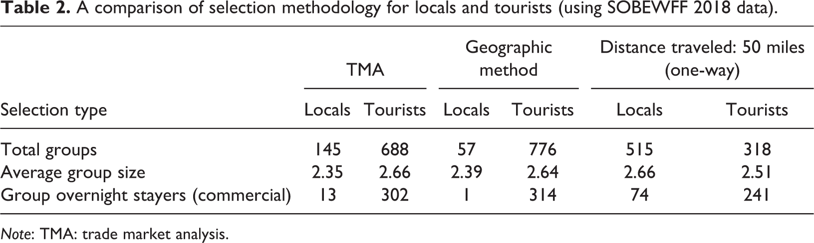
As mentioned above, the TMA analysis method was utilized in order to help differentiate local versus tourist (Davis et al., 2012; Warnick et al., 2015, 2017). The CTA (Miami Beach) consisted of 57 local groups. The CTA included all zip codes (4) in Miami Beach, Florida. Those zip codes on the mainland within a 10–15 mile/30-min drive were considered DTA. The DTA was comprised of 88 local groups for a grand total of 145 local groups. Because TMA is a new methodology for selecting locals and tourists, the authors chose to compare the TMA method to the distance traveled method (50 miles drive one-way) and the geographic method in which only Miami Beach zip codes were selected (see Table 2).

Table 2.

A comparison of selection methodology for locals and tourists (using SOBEWFF 2018 data).

	TMA		Geographic method		Distance traveled: 50 miles (one-way)
Selection type	Locals	Tourists	Locals	Tourists	Locals	Tourists
Total groups	145	688	57	776	515	318
Average group size	2.35	2.66	2.39	2.64	2.66	2.51
Group overnight stayers (commercial)	13	302	1	314	74	241

Note: TMA: trade market analysis.

These local groups (DTA and CTA) were surveyed on their spending along with tourist groups (overnight, day-trippers, casuals, and noncasuals) on their local spending in multiple industry categories. The estimated total spending for each group was calculated to show the difference between spending of each group classification at the Miami Beach festival. This calculation was made using the total number of groups multiplied by the average group expenditure for each spending category.

Each of the spending categories was assigned one of the 536 NAICS industry codes supplied on a bridge table from IMPLAN (Crompton et al., 2016; Daniels, 2004). For the EI, only the noncasual tourists were included in the analysis (about 25% of the actual groups who attended the festival). This noncasual group was identified by the question: “What was your main purpose for your visit to Miami Beach?” If respondent groups included SOBEWFF 2018 as their answer, they were included in the EI study. The average group spend for these noncasual tourists was multiplied by the number of estimated noncasual tourist groups at the festival. The final tally for each industry code was applied to the impact I/O method IMPLAN 4.3 in order to measure the EI of the 5-day festival (Leones et al., 1998).

Results

The surveying process returned 833 usable surveys (groups), 688 groups classified as tourists, and 145 groups classified as locals. Table 3 below indicates the average spend (economic significance) for each group type at the festival (overall expenditures of attendees in each spending category). Of the 688 total tourist groups, 315 (45.8%) indicated an overnight stay (commercial property, i.e. hotel), 38 (5.5%) indicated they were VFR, and 335 (48.7%) indicated “day-tripper.” The overnight tourists (US$3413.00 per group) and the day-trippers (US$571.54 per group) held significantly different expenditures on average per group (F (1, 650) = 152.02; p < 0.001). Lodging expense helped to fuel this difference in local spending (see Table 1).

Table 3.

Average group expenditures by category for locals and visitors (economic significance).

	Tourists (nonlocals)						Locals			Overall
	Day trip	Overnight (commercial)	VFR	Casuals	Noncasuals	All tourists	Locals (CTA)	Locals (DTA)	All locals	Total
Number of groups	335	315	38	483	205	688	57	88	145	833
Average group size	2.81	2.49	2.74	2.64	2.69	2.66	2.39	2.33	2.35	2.60
Overnight stays	0	3.17	4.34	1.23	2.79	1.71
Spending categories
Food and lodging
Lodging	US$0.00	US$1312.62	US$0.00	US$434.37	US$1001.33	US$603.31	US$50.88	US$130.68	US$99.31	US$515.58
Restaurants	US$108.67	US$633.26	US$454.82	US$277.89	US$574.01	US$366.12	US$237.37	US$232.95	US$234.69	US$343.24
Bars and nightclubs	US$47.68	US$195.25	US$148.70	US$91.82	US$192.06	US$121.69	US$119.12	US$41.48	US$72.00	US$113.04
Retail
Grocery stores and liquor stores	US$7.99	US$34.87	US$116.25	US$17.16	US$46.03	US$25.76	US$0.00	US$0.00	US$0.00	US$21.28
Pharmacies and beauty stores	US$5.07	US$19.85	US$61.93	US$11.68	US$19.59	US$14.04	US$0.00	US$0.11	US$0.07	US$11.61
Clothing/apparel stores	US$20.60	US$175.54	US$170.23	US$86.48	US$126.16	US$98.31	US$0.00	US$0.00	US$0.00	US$81.19
Gift and souvenir shops	US$0.60	US$31.49	US$20.68	US$12.57	US$24.19	US$16.03	US$0.00	US$0.00	US$0.00	US$13.26
Transport
Transportation: Car rental/Taxis/Buses/Uber/Lyft	US$22.41	US$117.56	US$94.20	US$60.71	US$92.97	US$70.32	US$33.16	US$52.10	US$44.66	US$65.85
Transportation: Parking	US$13.01	US$33.77	US$20.91	US$18.31	US$34.00	US$22.99	US$9.65	US$19.49	US$15.62	US$21.71
Gas stations	US$9.68	US$23.03	US$18.09	US$15.03	US$19.05	US$16.23	US$12.91	US$16.26	US$14.94	US$16.01
Leisure/entertainment
Tours and cruises	US$2.99	US$30.67	US$37.50	US$18.24	US$12.20	US$16.44	US$0.00	US$3.41	US$2.07	US$13.94
Museums	US$0.90	US$22.56	US$34.09	US$8.70	US$21.49	US$12.51	US$0.00	US$0.00	US$0.00	US$10.57
Sporting activities	US$1.79	US$7.75	US$25.00	US$2.67	US$13.90	US$6.02	US$0.00	US$0.00	US$0.00	US$4.97
Concerts and live events	US$1.97	US$12.19	US$25.68	US$5.43	US$12.44	US$7.52	US$0.00	US$0.00	US$0.00	US$6.21
SOBEWFF tickets	US$328.19	US$762.62	US$619.68	US$389.41	US$909.30	US$544.32	US$532.16	US$344.43	US$416.16	US$522.01
Total	US$571.54*	US$3413.00*	US$1847.77	US$1450.47*	US$3098.71*	US$1941.59	US$995.25	US$840.92	US$899.52	$1760.46
Average expenditure per person	US$203.39	US$1370.68	US$674.37	US$549.42	US$1151.94	US$729.92	US$416.42	US$360.91	US$382.77	US$677.10

Note: VFR: visiting friends and relative; CTA: convenience trade area; DTA: destination trade area.

* Significant at p < 0.05 level.

Those festival attendees who traveled to Miami Beach for reasons other than the festival (casual tourists n = 483) spent approximately US$1450.47 per group in the impact area while the noncasuals (n = 205) spent US$3098.71 per group. The casuals and noncasual per group spending was significantly different (F (1, 686) = 43.66; p < 0.001). Because Miami Beach has such a high number of tourists each year, the researchers expected many casual tourists at the festival. Although they may have planned their trip regardless of the festival, the attendance of the casuals still helped the overall success of the festival with average ticket sales at US$389.41 per group. Overall, all tourists to Miami Beach spent an average US$1941.59 per group, including US$729.92 on average per person.

The researchers applied TMA to separate the locals into a DTA area and CTA. As mentioned above, 145 locals and 688 tourists were identified via the TMA method. Of the 145 local groups in the sample, the Miami Beach CTA (57 groups) spent more on average than the DTA (88 groups) primarily on tickets and bars/nightclubs. This relationship difference (approximately US$154 per group) was not significant (F (1, 145) = 0.005; p > 0.05). Thus, the DTA was confirmed to behave similarly in their spending outcomes to the CTA. CTA group expenditures equaled US$995.25 per group, while DTA expenditures equaled US$840.92 per group. Overall, average group expenditures (including both locals and tourists) were US$1760.46 per group or US$671.93 per person.

Direct, indirect, and induced value-added impacts were then calculated, utilizing the estimated total expenditures for each spending category and NAICS code. Of the 833 surveys collected, 205 (24.6%) indicated that their groups visited Miami Beach specifically for the festival (noncasual tourists). Of the 205 noncasual groups, 23 of the groups did not spend the night in the Miami Beach area. Thus, of the 205 noncasual groups, 182 (89%) were overnight stays and 23 (11%) were day-trippers. Of the 182 overnight stays, 12 of the groups were VFR. Thus, 170 of the 205 noncasual tourist groups stayed in commercial lodging. An estimated 23,143 groups attended SOBEWFF 2018 based on data provided by festival organizers. Of the total groups, 5695 groups (or 24.6% of 23,143) were allocated to the noncasuals to be measured in the IMPLAN model. The average expenditure for the noncasual groups was calculated and then multiplied by the total noncasual group attendees (5695) to attain a total expenditure calculation for each industry category. For instance, it was estimated that the total spend on hotels by noncasuals was US$5.7 million. The EI for Miami Beach via direct output for all the expenditure categories listed above included US$16.8 million. Hotel spending and festival spending were among the largest direct impacts of the festival (more than US$5 million each). The indirect effects of the festival include festival organizers paying staff/event planners and marketers to plan and promote the festival. Suppliers for the special event need to be paid, and space on the beach and venue space at some of the hotels need to be rented (all indirect effects). The induced effects include those paid to work the festival, hotels, restaurants, gift shops, and so on using their wages to spend money on local businesses. The total sales output (including indirect and induced) equaled US$25.5 million (see Table 4). Attendee spending and total industry output for the industries in Miami Beach are listed below. Only the directly affected industries are shown in Table 4.

Table 4.

Noncasual tourist spending and total industry output for the 2018 SOBEWFF at Miami Beach, Florida.

Code	Industry	Attendee spending	Indirect ($)	Induced ($)	Total ($)
499	Hotels	US$5,702,584.07	US$46,962.76	US$87,783.17	US$5,837,330.00
491	Festival ticket sales	US$5,178,449.61	US$143,248.72	US$9435.09	US$5,331,133.42
501	Restaurants	US$3,268,985.56	US$30,343.42	US$140,546.09	US$3,439,875.07
503	Bars and nightclubs	US$1,093,801.15	US$61,902.75	US$58,707.02	US$1,214,410.92
412	Transportation	US$529,440.54	US$68,824.83	US$8116.33	US$606,381.70
403	Retail—clothing	US$329,054.21	US$11,412.45	US$68,558.28	US$409,024.95
512	Parking	US$193,657.78	US$4112.42	US$29,629.44	US$227,399.64
414	Tours and cruises	US$122,373.05	US$0.00	US$967.04	US$123,340.09
493	Museums, historical sites, zoos, and parks	US$79,174.39	US$8338.87	US$22,294.78	US$109,808.04
406	Gift/Souvenir shop	US$73,143.88	US$2,648.99	US$117,292.87	US$193,085.75
488	Concerts/Comedy shows/Concerts	US$70,840.24	US$19,201.39	US$21,703.76	US$111,745.39
400	Grocery stores/Liquor/Wine shops	US$69,451.22	US$19,104.95	US$10,449.18	US$99,005.35
496	Sporting activities (golf/water sports)	US$66,113.12	US$7595.13	US$33,411.55	US$107,119.80
401	Pharmacies/Beauty stores	US$35,803.91	US$10,682.20	US$58,419.21	US$104,905.32
402	Gas stations and convenience stores	US$15,842.55	US$3134.88	US$17,119.20	US$36,096.63
	Total	US$16,828,715.00	US$4,022,882.00	US$4,656,153.00	US$25,507,750.00

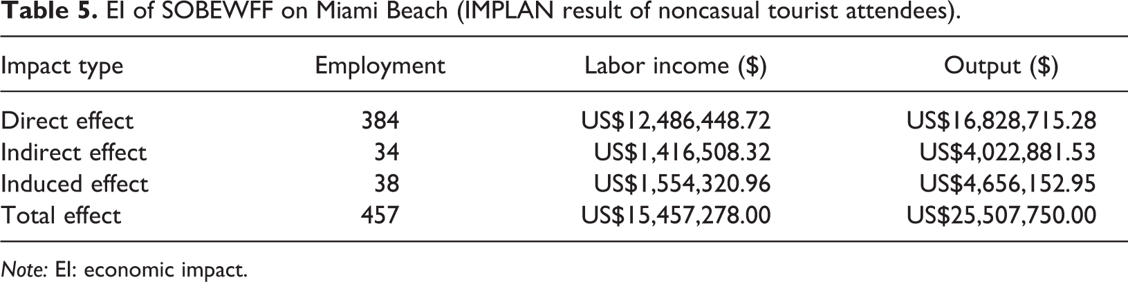
Researchers calculated the total EI of noncasual tourist attendees at SOBEWFF 2018 on the area defined as Miami Beach, Florida (for the CTA) and the surrounding area (DTA) using TMA (see table 5). A total of US$25.51 million in economic activity was generated in 2018 because of noncasual tourist spending on SOBEWFF. This total of US$25.51 million includes US$16.83 million in direct noncasual tourist spending on SOBEWFF, hotels and lodging, retail, restaurants, and transportation. Additionally, indirect economic activity of US$4.02 million in indirect spending occurred resulting from business expenditures on supplies and other operating expenses related to SOBEWFF, hotels, restaurants, retail, and transportation businesses in the area. Last, US$4.66 million in induced spending as a result of the multiplier effect of the spending of employee incomes occurred in the impact area (Alward et al., 1992; Shafer and Upneja, 2002). The total EI multiplier for Miami-Dade County was estimated by the IMPLAN model to be 1.70. Thus, for every US$1.00 spent directly by visitors to SOBEWFF, an additional US$0.70 in economic activity is generated throughout the EI area.

Table 5.

EI of SOBEWFF on Miami Beach (IMPLAN result of noncasual tourist attendees).

Impact type	Employment	Labor income ($)	Output ($)
Direct effect	384	US$12,486,448.72	US$16,828,715.28
Indirect effect	34	US$1,416,508.32	US$4,022,881.53
Induced effect	38	US$1,554,320.96	US$4,656,152.95
Total effect	457	US$15,457,278.00	US$25,507,750.00

Note: EI: economic impact.

Total payroll generated for Miami Beach equaled US$15.46 million. This US$15.46 million in total employee income comprised US$12.49 million in direct employee paychecks in the impact area (generated by direct spending by visitors on SOBEWFF, hotels and lodging, retail, restaurants, and transportation). Additionally, US$1.42 million in additional payroll was generated from indirect employee incomes of workers in other businesses providing supplies and other operating goods and services related to SOBEWFF, restaurants, hotels, and retail. Last, US$1.55 million of induced worker income was generated because of the multiplier effect of direct and indirect income spent in the local impact area (Miami-Dade County).

A total of 457 jobs were created resulting from visitor spending on SOBEWFF in 2018. These 457 jobs are considered full-time, annual-equivalent jobs (some are part-time seasonal jobs converted to full-time, full-year equivalent jobs). These 457 jobs include 384 jobs generated directly by direct visitor spending at SOBEWFF, hotels and lodging, restaurants, retail, and transportation businesses. Additionally, 34 indirect jobs were generated because of business expenditures on supplies and other operating expenses which help support occupations in other local businesses (hotels, restaurants, retail). Lastly, 38-induced jobs were created because of the multiplier effect of worker paychecks spent in the local economy (Beckman et al., 2012; Morse, 2012).

Discussion: TMA

In the past, EI studies have identified “locals” as those residing within specific zip codes (geographic method) or those traveling between 50 miles and 150 miles one-way (distance traveled) (Beckman et al., 2013; Crompton et al., 2001). As a contrast, TMA analysis utilizes both of these inputs, as well as other factors including drive time, geographic features of the impact area, retail/shopping mix of the impact area, and destination attractions (Davis et al., 2012). Within the literature, only one other study has used TMA to identify tourists and locals in an EI study (Warnick et al., 2015). For this TMA process, the “CTA” of the destination and the “DTA” of the destination were distinguished. The CTA (Miami Beach, Florida) is located in the impact area of the event and refers to the area in which the local population will go to shop, purchase gas, buy groceries, and get their hair done (Davis et al., 2012). The DTA refers to the area (radius) in which those will travel to the destination for attractions, major products, and services (Davis et al., 2012).

For the current study, the geographic characteristics of the impact area factored heavily in the selection of the CTA. Miami Beach, often known as “South Beach,” is a city with a population of 91,917 people (Anon, 2017b). It is a geographically diverse island separate from the mainland US and Miami. The island boasts a reputation for excitement with its fancy restaurants, cafes, bars, nightclubs, beaches, and hotels. In fact, almost 16 million people for each year visit the Miami Beach area, which is more than the Great Smokey Mountains National Park—most visited national park in the United States (11 million tourists per year) (Anon, 2017a; Houston, 2008; Wobensmith, 2018). Because Miami Beach is such a draw for tourists, there is increased congestion due to traffic and often more “out of towners” visiting the local businesses than the locals. For this reason, and the geographic isolation of the island, the four Miami Beach zip codes (7 square miles) were selected as the “CTA” (Davis et al., 2012).

To travel Miami Beach from anywhere other than Miami Beach will take longer than 15 min regardless of the geographic distance. In addition to the CTA locals, some within a 10–15 mile/up to 30-min radius may occasionally visit Miami Beach for the sun, beach, expensive restaurants, nightclubs, and shop on Lincoln Road (Lincoln Mall). Those outside of the 30-min travel-time radius of the Miami beach area may seldom drive to Miami Beach due to the limited parking, cost, time associated with the travel, and pull of other attractions and commercial outlets (malls, restaurants, etc.). Hence, the researchers selected a 10–15 mile/up to 30-min travel-time radius as the “DTA.” The DTA was selected using ArcGIS to map the counties/areas surrounding Miami Beach that take 15–30 min to travel to Miami Beach on average. Most of the DTA is north of Miami Beach and on the mainland (west of Miami Beach). In addition to all the factors in the selection of the CTA and DTA, a key indicator in the proper selection of the DTA may be to compare the overall spending of the CTA and the DTA at an event. If the CTA and DTA do not have significantly different spending patterns and limited or zero commercial overnight stays, then a proper TMA differentiation of locals and tourists is supported.

Limitations

Researchers queried attendees on their total expenditures during their entire trip to Miami Beach. This included current and future estimated expenditures in various categories. We understand that attendees to some events at SOBEWFF may have different spending patterns than attendees to other events within the festival. Additionally, estimates of future expenditures may not have the same accuracy as estimations of prior expenditures (during their trip). Thus, the researchers may have obtained greater accuracy of group expenditures on the final day of the event rather than on the second day of the event when the surveying commenced. Tickets to SOBEWFF events were typically for a single event during a single day. Some festivals including music and arts festivals encourage multiday attendance by offering tickets for multiday admission to the event. Future studies should determine how many days attendees plan to attend a multiday event to determine the profile of these valuable attendees.

Conclusion

As recommended, the authors utilized a TMA technique to select locals and tourists to measure the EI of a special event (Warnick et al., 2017). This technique provided a viable new way in which to select and quantify locals and tourists in different markets. The authors found the TMA technique useful in a high-traffic urban area where at times it may take 90–120 min to travel 25–30 miles. Because of the complexity of TMA including various inputs such as drive time, geography, distance traveled, and business/shopping mix, this technique appears to measure spending patterns more accurately and improves the distinction of attendees (locals and tourists) over previous techniques (geographic and distance traveled). As seen in Table 2, if the geographic method had been utilized, a majority of the festival attendee groups would have been considered “tourist” (93.2%). In this method, only 57 local groups were identified utilizing 4 Miami Beach zip codes. If the distance traveled method had been used, the percentage of groups considered tourist would have been considerably lower at 318 groups (38.2%). Of the 515 local groups identified in the distance traveled method, 74 of these groups purchased lodging in Miami Beach. This contrasts with the TMA method, in which only 13 of the 145 local groups purchased lodging in Miami Beach. These 13 overnight stays among the 145 local groups are another validation of the proper application of the TMA method (in addition to the similar spending patterns of DTA and CTA groups). Additionally, expenditure patterns of attendees from the CTA and DTA were found to be statically indifferent, thus confirming that both groups are indeed “locals” and should not be erroneously counted as tourists. After comparing the three differentiation methods for locals and tourists, it is recommended that future studies utilize the TMA method in the selection of tourists and locals for more accurate and precise results (influenced by the diverse inputs involved) in differentiation and EI analysis. Geographic method and distance traveled method each utilize a “one size fits all” type of selection for locals and tourists ignoring other factors. TMA can adapt to these varied factors including geographic features (mountains, rivers, and oceans), drive time, population density, and business/market mix.

After arranging locals and tourists through TMA, researchers depicted the spending patterns (economic significance) of different group classifications among these newly distinguished tourists (overnight, day-tripper, VFR, casuals, and noncasuals) and locals (CTA and DTA). An analysis of variance was employed to group expenditures and overnight stays to determine whether the groups were dissimilar at the p < 0.05 level. Stayovers (overnight tourists) had significantly different (US$3413.00) group spending than the day-tripper tourist group (US$571.54) spending (see Table 3). Those groups who stayed overnight spent more money in every category including lodging, restaurants, and bars (and had the largest impact in terms of average group expenditures). Additionally, casuals (US$1450.47) and noncasuals (US$3098.71) had significantly different group spending. This is partly due to a significant difference in average overnight stays (1.23 overnight stays for casuals and 2.79 overnight stays for noncasuals). Thus, hotel spending and ticket sales were higher with the noncasuals than the casuals.

The high average spending per overnight tourist group (US$3413.00) during the Miami Beach trip is largely due to the nature of the hotel industry in Miami Beach. Of the 199 hotels in Miami Beach, 141 of the 199 hotels are upscale (54), upper upscale (57), or luxury class (30). Therefore, these 141 independent hotels or chains have high annual room rates, ranging from US$150 to more than US$300 on average (Hood and Vinson, 2018). During peak times, such as during SOBEWFF, the 199 properties in Miami Beach averaged a rate of around US$430 per night for Friday and Saturday night during the festival. A four-hotel segment including luxury class hotels averaged over US$800 per night over the same time period (February 23 and February 24) (Hood and Vinson, 2018). Additionally, there are many high-end shops, restaurants, and bars located along the beach and Lincoln road.

This study confirmed that overnight tourists were significantly more valuable to the Miami Beach community than the day-trippers (in every spending category). These overnight tourists included those VFR. While VFRs were relatively low in this study (only 38 VFR groups identified), they stayed longer on average than any other classification (4.34 nights) and spent more in some categories on average than commercial overnight stayers (grocery stores, pharmacies, tours, museums, sporting activities, and live events). Destination marketing organizations should consider providing package deals on their website including hotel stays, tickets to the festival, restaurant vouchers, tours, and so on to help encourage tourists to stay multiple nights, impacting the local community on a greater scale (Beckman and Chang, 2018). Residual spending for these overnight stays is beneficial and most profitable for the destination.

It is important for stakeholders to know the EI of an event on a community; therefore, it can be fully supported (Ap and Crompton, 1993). To determine this EI, noncasual tourists were surveyed on their estimated spending on an array of industry-spending categories applicable to the local area (Miami Beach) inside and outside the event. The researchers showed the impact of this event on Miami Beach utilizing an I/O model. I/O models such as IMPLAN provide an accurate estimate of the direct and indirect value-added effects of an event (Chhabra, 2007; Lacher and Oh, 2012; Rose, 1998). Thus, IMPLAN was applied to the 2018 South Beach Wine and Food Festival. According to IMPLAN, the total sales output for the 2018 SOBEWFF was US$25.5 million. This in turn produced labor income of US$15.46 million and created 457 jobs in the impact area surrounding Miami Beach, Florida. The previously reported positive impacts of multiday special events and festival events are confirmed in this study.

Future research should continue to apply TMA on urban destinations with considerable amounts of annual tourists. Many cities consist of several different shopping districts, and consequently there are areas that may be geographically close, but residents of these areas may rarely travel to that district (or trade market) without the incentive of a festival or special event. In this instance, it is the strong recommendation of the authors to consider including TMA differentiation of locals and tourists in future impact analysis. This method should be applied carefully as one strength (and weakness) of TMA is that it requires a more profound understanding of the local economy, travel patterns, geography, and business mix. For instance, traffic patterns in a major metro area may define shopping patterns differently (in different cities and regions depending on business mix and tourism). Researchers utilizing TMA should take note of the differences and adapt these unique characteristics to the TMA method.

Footnotes

Declaration of conflicting interests

The author(s) declared no potential conflicts of interest with respect to the research, authorship, and/or publication of this article.

Funding

The author(s) received no financial support for the research, authorship, and/or publication of this article.

ORCID iD

Eric Beckman

References

Alward

Siverts

Taylor

. (1992) Micro IMPLAN, User’s Guide, Version 91-F. Fort Collins: USDA Forest Service, Land Management Planning Systems Group.

Andersson

Lundberg

(2013) Commensurability and sustainability: triple impact assessments of a tourism event. Tourism Management 37: 99–109.

Anon (2017a) Park Statistics. National Park Service. Available at: https://www.nps.gov/grsm/learn/management/statistics.htm (accessed 3 July 2018).

Anon (2017b) United States Census. Available at: https://factfinder.census.gov/faces/nav/jsf/pages/community_facts.xhtml?src=bkmk.https://www.nps.gov/grsm/learn/management/statistics.htm (accessed 7 July 2018).

Crompton

(1993) Residents’ strategies for responding to tourism impacts. Journal of travel research 32(1): 47–50.

Auld

McArthur

(2003) Does event-driven tourism provide economic benefits? A case study from the Manawatu region of New Zealand. Tourism Economics 9(2): 191–201.

Baade

Matheson

(2004) The quest for the cup: assessing the economic impact of the world cup. Regional Studies 38(4): 343–354.

Backer

(2007) VFR travel: an examination of the expenditures of VFR travellers and their hosts. Current Issues in Tourism 10(4): 366–377.

Backer

Leisch

Dolnicar

(2017) Visiting friends or relatives? Tourism Management 60: 56–64.

10.

Beckman

Chang

(2018) Consumer preference and willingness to pay for the tourism packages: a conjoint study of a rural destination. Business and Management Studies 4(2): 10–16.

11.

Beckman

Kumar

Kim

(2013) The impact of brand experience on downtown success. Journal of Travel Research 52(5): 646–658.

12.

Beckman

Morse

Costello

(2012) Economic Impact of Whitewater Rafting on the Ocoee River. Graduate Research Coloquim: Department of Retail Hospitality and Tourism Management 1: 6–8.

13.

Blichfeldt

Halkier

(2014) Mussels, tourism and community development: a case study of place branding through food festivals in Rural North Jutland, Denmark. European Planning Studies 22(8): 1587–1603.

14.

Bonn

Harrington

(2008) A comparison of three economic impact models for applied hospitality and tourism research. Tourism Economics 14(4): 769–789.

15.

Bowker

Bergstrom

Gill

(2007) Estimating the economic value and impacts of recreational trails: a case study of the Virginia creeper rail trail. Tourism Economics 13(2): 241–260.

16.

Bracalente

Chirieleison

Cossignani

. (2011) The economic impact of cultural events: the Umbria Jazz music festival. Tourism Economics 17(6): 1235–1255.

17.

Çela

Knowles-Lankford

Lankford

(2007) Local food festivals in northeast Iowa communities: a visitor and economic impact study. Managing Leisure 12(2–3): 171–186.

18.

Cheung

Mak

Dixon

(2016) Elite active sport tourists: economic impacts and perceptions of destination image. Event Management 20(1): 99–108.

19.

Chhabra

(2007) Estimating benefits and costs of casino gambling in Iowa, United States. Journal of Travel Research 46(2): 173–182.

20.

Chhabra

Sills

Cubbage

(2003) The significance of festivals to rural economies: estimating the economic impacts of Scottish Highland Games in North Carolina. Journal of Travel Research 41: 421–427.

21.

Croes

Severt

(2007) Research report: evaluating short-term tourism economic effects in confined economies - conceptual and empirical considerations. Tourism Economics 13(2): 289–307.

22.

Crompton

(2006) Economic impact studies: instruments for political shenanigans? Journal of Travel Research 45(1): 67–82.

23.

Crompton

(2010) Measuring the Economic Impact of Park and Recreation Services. Ashburn: National Recreation and Park Association.

24.

Crompton

Jeong

Dudensing

(2016) Sources of variation in economic impact multipliers. Journal of Travel Research 55(8): 1051–1064.

25.

Crompton

Lee

Shuster

(2001) A guide for undertaking economic impact studies: the Springfest example. Journal of Travel Research 40(1): 79–87.

26.

Daniels

(2004) Beyond input-output analysis: using occupation-based modeling to estimate wages generated by a sport tourism event. Journal of Travel Research 43(1): 75–82.

27.

Daniels

Norman

Henry

(2004) Estimating income effects of a sport tourism event. Annals of Tourism Research 31(1): 180–199.

28.

Davis

Clark

Pesch

(2012) Downtown and Business District Market Analysis. Available at: https://fyi.uwex.edu/downtown-market-analysis/ (accessed 25 July 2018).

29.

Diedering

Kwiatkowski

(2015) Economic impact of events and festivals on host regions - Methods in practice & AMP; potential sources of bias. Polish Journal of Sport and Tourism 22(4): 247–252.

30.

Dwyer

Forsyth

(1998) Economic significance of cruise tourism. Annals of Tourism Research 25(2): 393–415.

31.

Fourie

Santana-Gallego

(2011) The impact of mega-sport events on tourist arrivals. Tourism Management 32(6): 1364–1370.

32.

Getz

(1989) Special events: defining the product. Tourism Management 10(2): 125–137.

33.

Hall

(2000) The tourist and economic significance of Antarctic travel in Australian and New Zealand Antarctic gateway cities. Tourism and Hospitality Research 2(2): 157–169.

34.

Herrero

Sanz

JÁ

Devesa

. (2006) The economic impact of cultural events. European Urban and Regional Studies 13(1): 41–57.

35.

Hollows

Jones

Taylor

. (2014) Making sense of urban food festivals: cultural regeneration, disorder and hospitable cities. Journal of Policy Research in Tourism, Leisure and Events 6(1): 1–14.

36.

Hood

Vinson

(2018) STR Trend Report for Miami Beach: February 2018. Hendersonville, TN: STR SHARE Center.

37.

Houston

(2008) The economic value of beaches: a 2008 update. Shore and Beach 76(3): 22–26.

38.

Hunt

Layne

(1991) Evolution of travel and tourism terminology and definitions. Journal of Travel Research 29(4): 7–11.

39.

Josiam

Kinley

Kim

(2005) Involvement and the tourist shopper: using the involvement construct to segment the American tourist shopper at the mall. Journal of Vacation Marketing 11(2): 135–154.

40.

Kemper

Popp

Miller

(2008) Regional growth and beaver lake: a study of recreation visitors. Tourism Economics 14(2): 409–426.

41.

Kim

Dombrosky

(2016) Economic Impact of Small Scale Event to the Local Economy: Case of Canfield Fair. Journal of Tourism Insights 7(1): 1–10.

42.

Kim

Miller

(2017) An economic model comparison of EMSI and IMPLAN: case of mistletoe marketplace. Tourism Economics 23(5): 1124–1130.

43.

Kirillova

Bordelon

Pearlman

(2014) A comparison of expenditures between New Orleans volunteer and leisure tourists: implications for sustainability. Tourism Analysis 19(2): 173–184.

44.

Kwiatkowski

Diedering

Oklevik

(2018) Profile, patterns of spending and economic impact of event visitors: evidence from Warnemünder Woche in Germany. Scandinavian Journal of Hospitality and Tourism 18(1): 56–71.

45.

Lacher

(2012) Is tourism a low-income industry? Evidence from three coastal regions. Journal of Travel Research 51(4): 464–472.

46.

Lee

Taylor

(2005) Critical reflections on the economic impact assessment of a mega-event: the case of 2002 FIFA World Cup. Tourism Management 26(4): 595–603.

47.

Lee

Mjelde

Kwon

(2017) Estimating the economic impact of a mega-event on host and neighbouring regions. Leisure Studies 36(1): 138–152.

48.

Lee

Arcodia

(2011) The role of regional food festivals for destination branding. International Journal of Tourism Research 13: 355–367.

49.

Leones

Colby

Crandall

(1998) Tracking expenditures of the elusive nature tourists of southeastern Arizona. Journal of Travel Research 36(3): 56–64.

50.

Loomis

(2007) Correcting for on-site visitor sampling bias when estimating the regional economic effects of tourism. Tourism economics 13(1): 41–47.

51.

Loomis

Caughlan

(2006) The importance of adjusting for trip purpose in regional economic analyses of tourist destinations. Tourism Economics 12(1): 33–43.

52.

Masberg

(1998) Defining the tourist: Is it possible? A view from the convention and visitors bureau. Journal of Travel Research 37(1): 67–70.

53.

Matheson

(2009) Economic multipliers and mega-event analysis. International Journal of Sport Finance 4(1): 63–70.

54.

McGrath

Primm

Lafe

(2017) Heritage tourism’s economic contribution. Tourism Economics 23(5): 1131–1137.

55.

Meretse

Mykletun

Einarsen

(2016) Participants’ benefits from visiting a food festival – the case of the Stavanger food festival (Gladmatfestivalen). Scandinavian Journal of Hospitality and Tourism 16(2): 208–224.

56.

Morrison

Verginis

O’Leary

(2000) Reaching the unwanted and unreachable: an analysis of the outbound long haul German and British visiting friends and relatives market. Journal of Tourism and Hospitality Research 2(3): 214–231.

57.

Morse

(2012) The Estimated Economic Impacts of Ocoee River Whitewater Rafting on the Local Economy. Knoxville, TN: University of Tennessee.

58.

Orens

Seidl

(2009) Working lands and winter tourists in the rocky mountain west: a travel cost, contingent behaviour and input-output analysis. Tourism Economics 15(1): 215–242.

59.

Preuss

(2004) Calculating the regional economic impact of the Olympic games. European Sport Management Quarterly 4(4): 234–253.

60.

Preuss

(2011) A method for calculating the crowding out effect in sport mega-event impact studies: the 2010 FIFA world cup. Development Southern Africa 28(3): 367–385.

61.

Rose

(1998) The Regional Economic Impacts of Casino Gambling: Assessment of the Literature and Establishment of a Research Agenda, A. Houston: Rose and Assoc.

62.

Sánchez

Fernández

Lara

JÁS

(2017) Economic impact of a religious and tourist event: a Holy Week celebration. Tourism Economics 23(6): 1255–1274.

63.

Scott

Chhabra

(2017) Economic viability of heritage festivals in Wickenburg, Arizona (USA). Anatolia 28(3): 432–443.

64.

Shafer

Upneja

(2002) Economic benefits of sport fishing and angler wildlife watching in Pennsylvania: revisited. Journal of Travel Research 41(2): 212–213.

65.

Smith

Costello

(2009) Segmenting visitors to a culinary event: motivations, travel behavior, and expenditures. Journal of Hospitality Marketing and Management 18(1): 44–67.

66.

Stoddard

Davé

Evans

. (2006) Economic impact of the arts in a small US county. Tourism Economics 12(1): 101–121.

67.

Stynes

White

(2006) Reflections on measuring recreation and travel spending. Journal of Travel Research 45(1): 8–16.

68.

Tien

Lin

(2011) The economic benefits of mega events: a myth or a reality? A longitudinal study on the Olympic games economics and finance. Journal of Sport Management 25: 11–23.

69.

Tohmo

(2005) Economic impacts of cultural events on local economies: an input – output analysis of the Kaustinen folk music festival. Tourism Economics 11(3): 431–451.

70.

Warnick

Bojanic

Mathur

. (2011) Segmenting event attendees based on travel distance, frequency of attendance, and involvement measures: a cluster segmentation technique. Event Management 15(1): 77–90.

71.

Warnick

Bojanic

Cartier

(2013) Economic impact research: review of measurement techniques in a special event. In: Tourism Travel and Research Association: Advancing Tourism Research Globally. Kansas City, MO, pp. 1–14.

72.

Warnick

Bojanic

Cartier

(2017) A comparison of economic impact measurement techniques for a tourism special event. Journal of Travel Research 56(5): 578–592.

73.

Warnick

Bojanic

(2015) Using a trade market analysis technique to refine measurements for economic impact analysis of special events. Journal of Travel Research 54(1): 52–65.

74.

West

(1993) Economic significance of tourism in Queensland. Annals of Tourism Research 20(1): 490–504.

75.

Wobensmith

(2018) Greater Miami and beaches research and statistics. Available at: http://partners.miamiandbeaches.com/tools-and-resources/research-and-statistics (accessed 10 July 2018).

76.

KIm

ChEN

CIC

. (2012) Are you a tourist? Tourism definition from the tourist perspective. Tourism Analysis 17(4): 445–457.