Tourist arrivals versus tourist expenditures in modelling tourism demand

Abstract

In empirical research, aggregate tourist arrivals and tourist expenditures are often indistinctly used as measures of tourism demand, depending on the aim of the analysis or, simply, on the availability of data. However, when a literature review was conducted, we found differences in the estimated elasticities, accordingly to the measure that was used. This article investigates these two measures, exploring the theoretical link between them in the context of tourism demand modelling at a destination level. Having established the theoretical connection between the two variables with implications on the estimated elasticities, we estimate tourism demand models using international arrivals and tourist expenditures for 191 countries from 1998 to 2016, providing evidence for the theoretical connection. Our results show that when both tourist demand measures are used, the estimated elasticities may differ.

Keywords

average expenditures tourist arrivals tourist expenditures world tourism trends

Introduction

In recent literature on tourism economics, attention has focussed on tourism demand modelling. Empirical applications have mainly centred on methodological issues and the study of specific determinants. However, surprisingly, given the theoretical and empirical consequences of the dependent variable that is chosen, there has been little discussion of the implications of the choice of tourism demand measure that is used. During recent decades, different literature reviews and meta-analyses have confirmed that tourist arrivals and tourist expenditures are the most recurrent variables used in tourism demand modelling exercises (Crouch, 1994a,b, 1995; Lim, 1997a,b, 1999; Peng et al., 2014, 2015; Song and Li, 2008; Witt and Witt, 1995). If we refer to one of the most recent reviews, based on 195 studies comprising a total of 2833 estimated demand elasticities, Peng et al. (2015) show that tourist arrivals were used in 64.9% of all cases and tourist expenditure in 21.4%.

According to economic theory, the demand variable used to estimate a demand equation should represent the quantity of the demanded good (Varian, 2010). However, because tourism is made up of a combination of several separate goods and services, definable in monetary terms, as opposed to a conventionally measured quantity, finding an appropriate measure is a controversial issue. On the one hand, in real monetary terms, tourism demand represents an amount of expenditure and a certain quality standard (Smeral, 1988), captured by an implicit price. On the other hand, the number of tourists does not reflect changes in the average length of stay and neither does it capture changes in average expenditures (Crouch, 1994a).

The meta-regression results obtained by Peng et al. (2015) show that when tourist expenditures are used as a measure of international demand, a higher price elasticity is found and an ‘unexpectedly’ significant negative effect on estimates of income elasticities occurs in some cases. In demand forecasting, Song et al. (2010) compared the use of tourist arrivals and tourist expenditures in the context of Hong Kong econometric time series modelling, finding significant differences in the most important determinants of both variables for the case study under question.

Though it is possible to argue that the use of tourist arrivals or tourist expenditures will depend on whether the decision maker’s objective is to maximize tourist arrivals or expenditures, it is important not to overlook the fact that these variables are linked from a theoretical point of view: an issue that could have repercussions on the empirical results. From a microeconomic perspective, Aguiló et al. (2017), Downward and Lumsdon (2000, 2003) and Fleischer and Rivlin (2009) differentiated between quality and quantity in studies of individual daily tourist expenditures and the length of stay, demonstrating the existence of a relationship between these two variables and total individual tourist expenditure. However, to the best of our knowledge, no one has tried to transpose the implications of these interactions demonstrated at an individual level to an aggregate level, despite the widespread use of aggregate tourism demand models in the literature on tourism.

Consequently, in the light of the above gap, comprehensive research is needed on the underlying relationship that helps to explain the differing demand estimation results obtained by the two variables and the impact of the selected demand measure on the estimation of the demand elasticities. This study aims to achieve this objective by investigating, first, the theoretical relationship between two aggregated demand models using tourist arrivals and tourist expenditures and, second, checking the theoretical findings in an empirical exercise modelling yearly international aggregate data at a national level from 191 countries during the period from 1998 to 2016. In this way, it extends the studies of Qiu and Zhang (1995), Sheldon (1993) and Song et al. (2010), who compared the use of tourist arrivals and tourist expenditures in tourism forecasting, but also previous reviews on tourism demand modelling, who have found differences in estimated elasticities depending on the use of expenditures or tourist as dependent variable, by analysing the underlying theory that relates the elasticities in two demand functions that use these two different dependent variables.

The remainder of this article is organized as follows: the next section investigates the relationship between aggregate tourist expenditures and aggregate tourist arrivals and the implications of this relationship on the estimated elasticities in regression models. The third section outlines the theoretical findings, using international tourism demand models at a worldwide level. The fourth section presents the empirical application and the fifth section the discussion of the empirical application. Finally, the sixth section outlines the conclusions.

Tourist expenditure: Tourist Arrivals × Average Tourist Expenditure

Total expenditures at a destination are an attractive starting point for destination managers aiming to evaluate the economic impact of tourism. A general standard theoretical model for studying the determinants of tourism demand to a particular destination, measured in terms of total tourist expenditures, can be represented as:

E_{j t} = f (X_{j t}^{k})

where $E_{j t}$ denotes the tourist expenditure at destination j during period t, and $X_{j t}^{k}$ denotes k determining variables related to destination j during the time period t. As Witt and Witt (1995) show, the functional form most commonly used to specify the relationship between tourist expenditures and their determinants is the power model, which assumes that the relationship between tourism demand and its determining variable is characterized by a constant elasticity. However, it is often found that, for some determinants, a constant elasticity is unacceptable (for instance for dummy variables). Therefore, the most common specification in the tourism demand literature has considered the double logarithmic form, in which coefficients are elasticities except for the coefficients of the dummy variables (Crouch, 1994a; Dogru et al., 2017; Peng et al., 2014). Analytically, taking the k1 subset of k determining variables with a constant elasticity and the k2 subset of k determining variables with a semilog relationship, the underlying model frequently assumed in tourism demand modelling can be expressed analytically as:

E_{j t} = e^{α} {(X_{j t}^{k 1})}^{β_{k 1}} e^{β_{k 2} X_{j t}^{k 2}} e^{μ_{j t}}

where α, β_k ₁ and β_k ₂ are parameters to be econometrically estimated, and $e^{μ_{j t}}$ is an error term assumed to be normal and identically distributed. For estimation purposes, equation (2) is usually transformed using natural logarithms to a better-known, more practical equation:

ln E_{j t} = α + \sum_{i = 1}^{k 1} β_{i} ln (X_{j t}^{i}) + \sum_{l = 1}^{k 2} β_{l} X_{j t}^{l} + μ_{j t}

Thus, α is known as the constant term, β_i are parameters that can be directly interpreted as elasticities and β ₁ are parameters that express how a unit increase in the determining variable is translated into an increase in percentage terms in tourism demand. It should be noted how equation (3) is quite similar to the formula used by Song et al. (2009: 2) when representing the aggregated demand function for the tourism product. In any case, from equation (3), the destination manager’s main task is to try to identify and quantify which specific variables can be included in X and to evaluate which of them can be modified with specific tourist policies so as to maximize tourist expenditure.

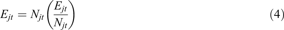
At this point, it is important to note that the total aggregate tourism demand, evaluated in terms of tourist expenditure, can be decomposed into the number of tourists and the average expenditure per tourist. Thus:

E_{j t} = N_{j t} (\frac{E_{j t}}{N_{j t}})

where $N_{j t}$ denotes the number of tourists and $(\frac{E_{j t}}{N_{j t}})$ the average expenditure per tourist. For a destination manager, it could be argued that the number of tourists $N_{j t}$ mainly captures the concept of ‘quantity’, while $(\frac{E_{j t}}{N_{j t}})$ somehow represents the concept of quality, in the sense that tourists with higher expenditures are expected to be related to higher quality tourism. Whatever the case, using natural logarithms in both parts of equation (4), we get

ln E_{j t} = ln N_{j t} + ln (\frac{E_{j t}}{N_{j t}})

Accordingly, from equations (3) and (5), it is possible to write:

ln N_{j t} + ln (\frac{E_{j t}}{N_{j t}}) = α + \sum_{i = 1}^{k 1} β_{i} ln (X_{j t}^{i}) + \sum_{l = 1}^{k 2} β_{l} X_{j t}^{l} + μ_{j t}

Furthermore, because of the linear relationship, after using the logarithm, we can consider the following decomposition:

ln N_{j t} = α^{B} + \sum_{i = 1}^{k 1} β_{i}^{B} ln (X_{j t}^{i}) + \sum_{l = 1}^{k 2} β_{1}^{B} X_{j t}^{l} + μ_{j t}

ln (\frac{E_{j t}}{N_{j t}}) = α^{A} + \sum_{i = 1}^{k 1} β_{i}^{A} ln (X_{j t}^{i}) + \sum_{l = 1}^{k 2} β_{1}^{A} X_{j t}^{l} + μ_{j t}

where equation (7) represents a traditional demand model in which the number of tourist arrivals is explained by the same set of k determining X variables, while equation (8) is a ‘demand’ model where average tourist expenditures are explained by the same set of determining variables. At this point, it is important to highlight how all these variables evaluated at country level are estimations that cannot be measured without errors that is an issue that can lead to reduced power, biased coefficients and erroneous inferences (de Haan et al., 2018). In any case, focusing our attention on the estimated parameters of equations (3), (7) and (8), as equation (3) can be obtained from the sum of equations (7) and (8), then the relationship between the estimated parameters can also be obtained from $α = α^{A} + α^{B}$ , $β_{i} = β_{i}^{A} + β_{i}^{B}$ and $β_{l} = β_{l}^{A} + β_{l}^{B}$ .

Therefore, the estimated parameters of a tourism demand model using total expenditures (β) should be different from the estimated parameters of a tourism demand model using total arrivals (β^B ) unless the considered determining variable has no effect on average tourist expenditures (β^A = 0).

Modelling international tourism demand at a destination level

Tourism demand at a destination can be affected by a wide range of factors. The theoretical model that supports tourism demand modelling literature is based frequently on consumer theory (Morley, 1992; Papatheodorou, 2001), and it assumes that the individual utility is derived from visiting different destinations as well as from the consumption of other services and goods. Thus, personal income and prices are introduced in the problem as a part of the budget constraint, while in the context of recreational demand, it is also common to consider site qualities as part of the determining function of the utility function (McConnell, 1992). Once the individual demands have been determined as a function of income, price and other site variables, the aggregated demand can be obtained through the consideration of all the residents of a particular origin (for instance, a country) visiting a particular destination (for instance, a country) during a certain period (for instance, a year). Although these simple statements entail some problems in their application regarding the macroeconomic aggregation (Morley, 1995; Morley et al., 2014), the literature review reveals how econometric modelling seeking to find dependent relationships between aggregated tourism demand and a set of macroeconomic explanatory variables has been the most popular approach in tourism demand modelling exercises (Crouch, 1994a; Peng et al., 2014).

According to the economic theory, the most included explanatory variables in empirical exercises have been income and prices (Crouch, 1994a; Peng et al., 2015). The income elasticity is generally greater than one, implying that tourism is regarded as a luxury good. The price of tourism is often also introduced in tourism demand models and, according to economic theory, it is negatively related to tourism demand. In general, the price elasticity displays a wider range of estimated values, probably because of the different components associated with tourism prices (Dogru et al., 2017; De Vita and Kyaw, 2013; Oh and Ditton, 2005; Rosselló, 2015).

Other potentially significant determinants that have been discussed in previous dynamic studies include prices in substitute or alternative destinations (Song and Wong, 2003; Witt and Witt, 1995); unemployment rates (Cho, 2001); income distribution and inequality (Morley, 1998); marketing and destination promotional expenditures (Crouch et al., 1992; Kulendran and Divisekera, 2007); incidence of infectious diseases (Rosselló et al., 2017); size of the population within the origin (Turner and Witt, 2001); trends in immigration patterns (Seetaram and Dwyer, 2009); political instability (Fourie et al., 2020; Santana-Gallego et al., 2019); extreme weather (Rosselló et al., 2011); one-off events (Fourie and Santana-Gallego, 2011; Smeral, 2008) and among others.

When destination managers try to understand the fundamental reasons why tourists choose a particular destination, instead of forecasting tourism demand, the time dimension and the dynamics of the tourism demand become less important in favour of the spatial variability. In other words, sometimes the main interests are trying to explain why tourists choose a specific destination (and which variables determine this choice) and not as much as their decisions change over time or evolve in the future. From this perspective, then, econometric models, based both on microeconomic and macroeconomic data, are superior (Song et al., 2009).

On the one hand, using survey data, microeconometric tourism demand modelling tries to identify the determinants of destination choice at the individual level. While personal income and tourism costs continue to be the key determinants, many other time-invariant factors can be involved, such as political stability at destination (Seddighi and Theocharous, 2002), the climate (Bujosa and Rosselló, 2013), the coastline (Lyons et al., 2009), personal motivations (Thrane, 2008) and other traditional socio-economic factors like age, gender, marital status, the household size and occupation (Brida and Scuderi, 2013; Eymann and Ronning, 1997). In addition to exploring destination choice, microeconometric modelling can also focus on tourist expenditures at a particular destination or other tourist behaviours, like the length of stay (Aguiló et al., 2017).

On the other hand, using macroeconomic variables, aggregate tourism demand models that focus on destination choice (not on the demand dynamics) have made a recent reappearance in literature, largely classed as ‘gravity models’ (Morley et al., 2014). These models aim to explain differing international tourism flows from/to different countries in relation to a set of explanatory variables associated with the origin/destination countries. Thus, rather like time series models, the higher the incomes of two countries, the bigger the expected tourism flows between them, while the higher the price of travel between two countries (mainly represented by distance), the lower the flows. Likewise, this will also be determined by numerous other variables referred to origin, destination or both, such as transport infrastructures (Khadaroo and Seetanah, 2008), climate and other geographical characteristics (Rosselló and Santana-Gallego, 2014), mutual agreements (Santeramo and Morelli, 2016), cultural and sociodemographic issues (Fourie and Santana-Gallego, 2013) or visa policies (Neumayer, 2010).

If the analysis of tourism demand is conducted at a destination level and we assume, as is often observed in international tourism databases, that the total tourist demand at a destination is known but that this demand’s country of origin is unknown (for instance, the total tourist expenditure to a specific destination country is observed but we do not know where this tourism demand comes from), then only variables related to the destination country can be included in the demand model. However, if data for different years is available, country-specific and year effects can be considered, thus obtaining the coefficients of all the variables of interest relating to the destination. We discuss this empirical question in the following section.

Empirical application

The data

For equations (3), (7) and (8) to be estimated, a database must be compiled that includes information on international expenditures (E), international tourist arrivals (N) and average expenditure per tourist (E/N) (the three variables to be used as dependent variables) and a set of potential determinants at a destination level (see Table 1 for a summarized list and the main descriptive statistics of the variables used in this study). These variables have been selected accordingly to previous literature analysed in previous sections. Here it is important to highlight how, because of the aggregated nature of the dependent variables, related to a specific destination country but without information about the origin country, only variables related to the destination can be included in the empirical exercise.

Table 1.

Descriptive statistics of the variables.

	Mean	Median	Maximum	Minimum	Standard deviation
E	5700.00	462.00	261,000.00	0.10	18,400.00
N	4913.10	866.00	95,676.00	1.00	11,568.25
E/N	1187.87	506.43	48,048.08	12.30	2924.70
GDPpc	13,064.49	4109.37	192,989.20	102.64	20,537.52
POP	32,431.52	5614.93	1,380,000.00	9.31	126,000.00
PPP	237.83	4.40	13,568.25	0.003	966.89
COAST	3813.77	440.00	202,080.00	0	15,777.52
SQKM	611.88	96.32	16,377.74	0.002	1768.44
TEMP	18.65	22.15	28.25	−5.35	8.34
WHS	5.15	2.00	53.00	0	8.83
VISA	32.66	23.50	99.00	0	22.17
NLBorders	2.92	3.00	16.00	0	2.70
Europe	0.25	0	1	0	0.43
Africa	0.28	0	1	0	0.45
Oceania	0.07	0	1	0	0.26
North America	0.12	0	1	0	0.32
South America	0.06	0	1	0	0.24
Asia	0.24	0	1	0	0.43

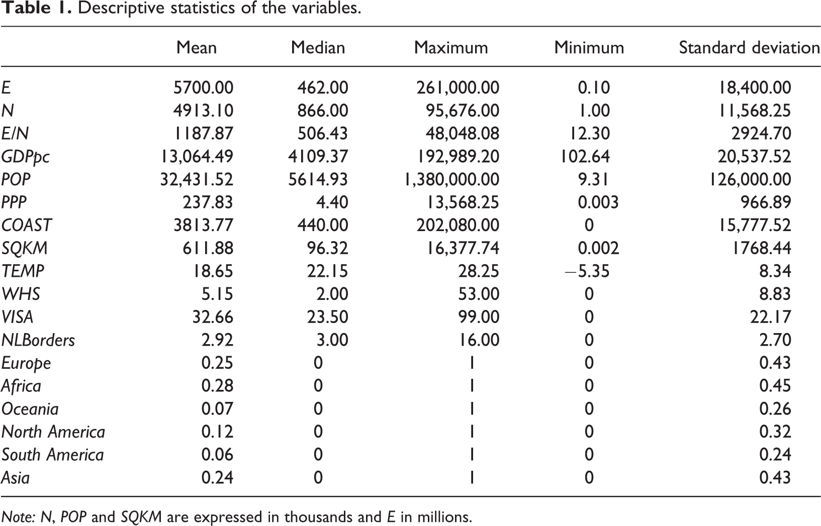
Note: N, POP and SQKM are expressed in thousands and E in millions.

Total international tourism expenditures to each country and total international tourist arrivals to each country is taken from the World Bank’s World Development Indicators (WDI) and was originally collected from the United Nations’ World Tourism Organization. Based on the available data for international tourism demand and the rest of the explanatory variables (explained below), a total of 191 countries from 1998 to 2016 are considered.

The explanatory variables included in the tourism demand models and taken also from the WDI (available free of charge online) are the following: the GDPpc or gross domestic product at purchaser prices in constant US$ divided by the midyear population. As in similar applications, the higher this indicator is, the higher the expected level of tourism, since the former is related to the level of development at the destination. POP is the national population, taken from the United Nations Population Division. The higher this indicator is, the higher the expected level of tourism, as this variable is related to tourist visits to friends and relatives. PPP is the purchasing power parity conversion factor, defined as the number of units of a country’s currency required to buy the same amounts of goods and services in the domestic market as the US dollar would buy in the United States. As a price indicator, the higher it is, the lower the expected level of tourism. In this case, it is important to note how the use of the exchange rate (in nominal or real terms), often used in similar exercises (Dogru et al., 2017; De Vita and Kyaw, 2013; Oh and Ditton, 2005), is not suitable because of the aggregated nature of our demand variables, referred to the total amount of expenditures or total amount of international arrivals to a specific destination, but without differentiating by origin.

Because we are focussing on tourism at a destination level, we also include different variables from different sources (all of them easily available free of charge online). They are COAST, the country coastline in kilometres, and SQKM, the country’s surface area in square kilometres from the CIA World Factbook; TEMP, the country’s average yearly temperature in degrees Celsius from the Tyndall Centre for Climate Change Research dataset; WHS, the country’s UNESCO World Heritage Sites and VISA, the tourist visa requirements for the destination country for tourism visits of a limited duration by visitors from worldwide source markets (100 = no visa required for visitors from all source markets, 0 = conventional visa required for visitors from all source markets), taken from the World Economic Forum’s Travel & Tourism Competitiveness Report and NLBorders, the country’s number of on-land borders, taken from the dataset of the Centre d’Etudes Prospectives et d’Informations Internationales. Lastly, we include dummy variables to control for the continent where the country is (Europe, Africa, Oceania, North America, South America and Asia, although the last one is used as the reference continent).

Estimation results

Considering the methodological indications and data availability above, we employ panel estimation methods. Given that panel estimation by fixed effects cannot be applied since the main variables of interest for a destination manager are time invariant and they would be dropped from the estimation, then we consider fixed effects ordinary least squares (OLSFE) panel estimation techniques, which incorporate country-specific and year fixed effects, thus obtaining the coefficients of all the variables of interest related to the destination. In any case, Hausman tests indicate that the fixed effect procedure is more appropriate than random effects. Additionally, by incorporating individual destination country fixed effects, we can control for unobserved heterogeneity (Anderson and vanWincoop, 2003; Kandogan, 2008).

The results of the estimated parameters using OLSFE corresponding to equations (3), (7) and (8), explaining international expenditures (E), international tourist arrivals (N) and average expenditure per tourist (E/N), respectively, are presented in Table 2 (showing the annual fixed effects in Table 3). The goodness of fit of the models is high in terms of the adjusted R-squared in the expenditure equation and tourist demand equations. In the case of the average expenditure equation, although the adjusted R-squared is lower, the F-statistic is very high and most of the coefficients used in the first two equations are significant, showing that when expenditure or tourist arrivals are used as the independent variables, the parameters of demand equations need not coincide.

Table 2.

OLSFE results.

	Ln(E)	Ln(N)	Ln(E/N)
Constant	−0.228	−0.982**	0.754
Ln(GDPpc)	0.988***	0.566***	0.422***
Ln(POP)	0.865***	0.229***	0.636***
Ln(SQKM)	−0.090***	0.241***	−0.331***
Ln(POP)/Ln(SQKM)	−0.033	1.745***	−1.779***
Ln(PPP)	−0.015***	−0.069***	0.055***
Ln(COAST)	0.008**	0.037***	−0.028***
TEMP	−0.050***	0.077***	−0.127***
TEMP²	0.001***	−0.003***	0.004***
Ln(WHS)	0.026	0.393***	−0.367***
VISA	0.005***	0.009***	−0.004***
NLBorders	−0.005	0.047***	−0.052***
Europe	0.014	−0.070	0.085
Africa	−0.141***	−0.058	−0.082***
Oceania	0.153	−0.938***	1.091***
North America	−0.302***	0.252***	−0.554***
South America	−0.219***	−0.681***	0.462***
Observations	2330	2330	2330
R-squared	0.923	0.792	0.364
Adjusted R-squared	0.922	0.789	0.355
S.E. of regression	0.569	0.779	0.895
Sum squared resid	743.8	1392.9	1839.8
F-statistic	806.5	257.0	38.8
Prob (F-statistic)	0	0	0

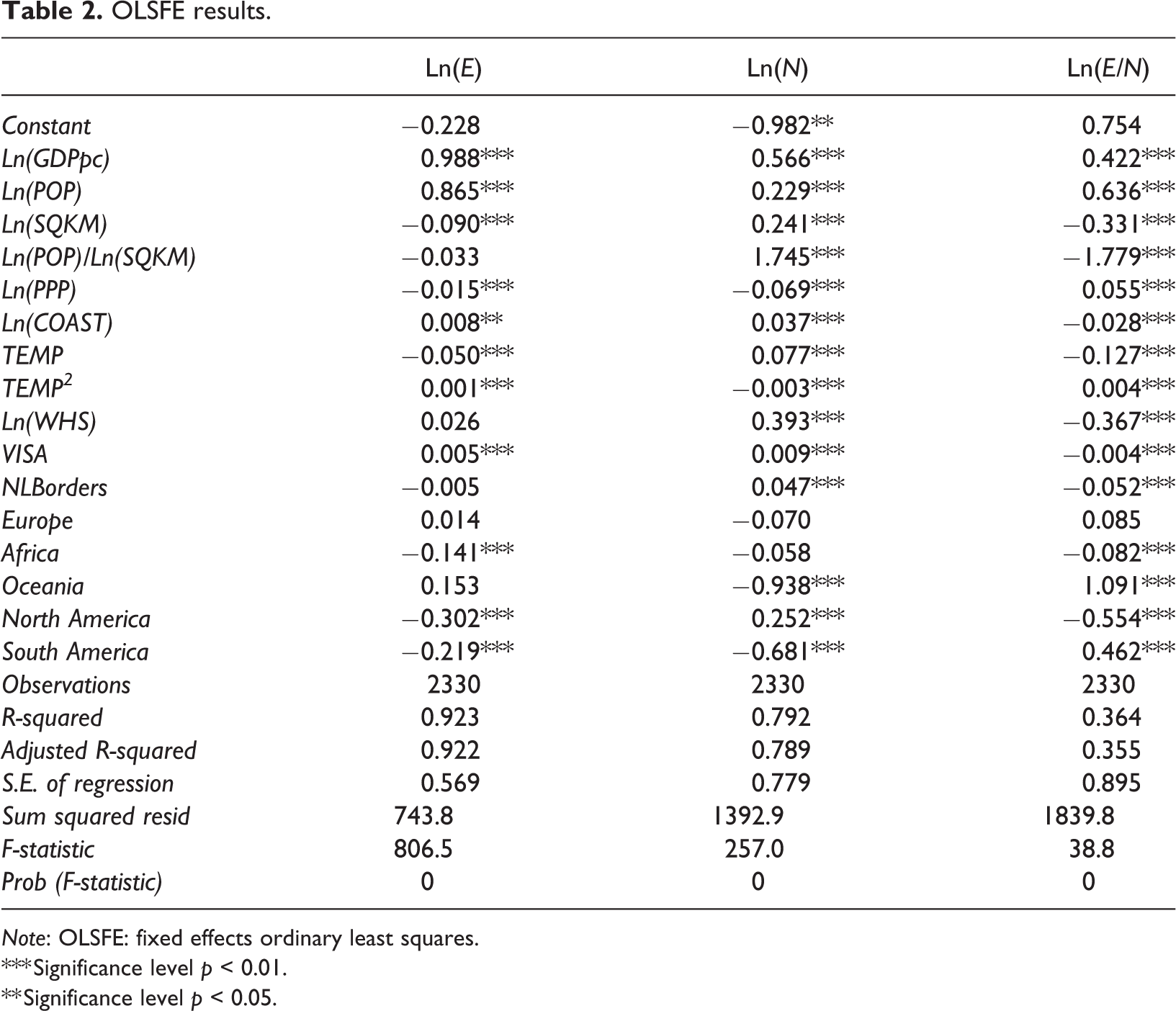
Note: OLSFE: fixed effects ordinary least squares.

*** Significance level p < 0.01.

** Significance level p < 0.05.

Table 3.

Annual fixed effects from OLSFE estimation.

	Ln(E)	Ln(N)	Ln(E/N)
Y_1999	0.022	0.051	−0.029
Y_2000	0.076	0.125	−0.049
Y_2001	0.072	0.147	−0.075
Y_2002	0.078	0.162	−0.084
Y_2003	0.035	0.144	−0.109
Y_2004	0.052	0.201	−0.149
Y_2005	0.070	0.222	−0.151
Y_2006	0.048	0.240	−0.192
Y_2007	0.059	0.238	−0.179
Y_2008	0.024	0.187	−0.163
Y_2009	−0.013	0.218**	−0.231**
Y_2010	−0.057	0.208**	−0.265**
Y_2011	−0.055	0.220**	−0.275**
Y_2012	−0.055	0.282***	−0.337***
Y_2013	−0.020	0.315***	−0.334***
Y_2014	0.004	0.376***	−0.372***
Y_2015	0.087	0.484***	−0.397***
Y_2016	0.145*	0.616***	−0.471***

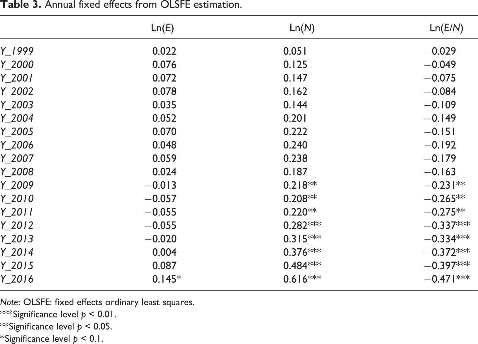
Note: OLSFE: fixed effects ordinary least squares.

*** Significance level p < 0.01.

** Significance level p < 0.05.

* Significance level p < 0.1.

As theoretically anticipated in the second section, the parameters of the demand equation measured in terms of expenditure (E) can be obtained by adding the parameters of the demand equation based on tourist arrivals (N) to the parameters of the demand equation using average expenditure per tourist as a measure (E/N). In other words, the impact of every determinant on total tourist expenditure can be explained by the impact of the number of tourists plus the impact of average tourist expenditure.

As expected, the estimation results show that the income in the destination country (GDPpc), used as a proxy for the level of development, has a positive relationship with tourism demand, whichever dependent variable is used. From the estimated parameters, it is possible to conclude that a 1% increase in the GDPpc at the destination is related to a 0.988% growth in tourism expenditure, which stems from a 0.566% increase in tourist arrivals and a 0.442% increase in average expenditure. Previous studies of tourism demand modelling have estimated an income elasticity of demand of over 1, showing that, as income rises, tourism consumers spend an increasing amount of their income on international travel (Peng et al., 2014). However, in the meta-analysis by Crouch (1996), although the mean income elasticity was 1.86, the standard deviation was 1.78, showing that many empirical applications obtained a value of between 0 and 1, indicating that tourism is a necessary good.

The population at the destination country (POP) is also related to the size of the tourism demand, whichever dependent variable is used. Thus, a 1% increase in the population at the destination is related to a 0.229% growth in tourist arrivals and a 0.636% growth in average expenditure, jointly representing a 0.865% increase in tourist expenditure there. In the case of the size of the country (SQKM), the larger the country, the higher the number of tourists. However, the size of the country is also negatively related to average expenditure, and because the negative effect is larger than the positive effect, the net effect on tourist expenditure is negative. The total effect of the population and size of the country is probably more complex. For this reason, we have used a combination of both variables Ln(POP)/Ln(SQKM) to proxy the effects of friends and relatives density. For this variable, although no significant effect was found for total expenditure, a positive relationship with total arrivals and a negative effect with average tourist expenditure were found, indicating that destinations with a high population density could be cheaper and receive more visits than ones with a low population density.

The price variable (PPP) is negatively related to tourism demand in the case of both expenditure and tourist arrivals. Thus, a 1% increase in the PPP variable is related to a 0.015% decrease in tourism expenditure and a 0.069% drop in tourist arrivals. However, it should be noted that a higher price is also related to a higher average expenditure. The effect of the length of the coastline (COAST) is also illustrative. On the one hand, it is positively related to a higher number of tourists and, on the other hand, it is negatively related to a lower average expenditure. Overall, the total effect on tourism expenditure is slightly positive.

Due to the use of the squared term, the effect of temperature on tourism demand reveals new results about this specific relationship. On the one hand, as found in previous literature (Hamilton et al., 2005; Hamilton and Tol, 2007; Rosselló and Santana-Gallego, 2014), an inverted u-shape is found in the relationship between the temperature at the destination and tourist arrivals, thus showing that the temperature there is positively related to tourist arrivals up to an optimal point after which it then becomes a negative factor. However, the relationship becomes u-shaped in the case of average expenditures and this same relationship is transferred to total expenditures, with the highest tourist expenditures being displayed at both extremes (at very cold and very hot destinations). This result should be related to the higher costs associated to keep tourists in comfort environments and other costs associated to food and other services provision. However, future investigations should confirm this outcome.

WHS and how easy it is to get a visa (VISA) are also interesting relationships to analyse due to the potential that managers have for intervening in and influencing these variables. In the case of WHS, the relationship has been captured assuming a constant elasticity (so taking logs in the independent variable). However, in the case of VISA, because of the index nature of the variable (and the difficulties in interpreting the results in terms of elasticity), the variable is included in levels. In any case, results not differ significantly for the consideration of the logarithms for both variables and the final specification is mainly motivated for the ease of interpretation of the results. Then, in both cases, it is found that an increase in the number of heritage sites and easier obtainment of a visa lead to an increase in the number of tourist arrivals. However, these two factors are also both related to a decrease in average tourist expenditures. The overall impact on total tourist expenditure is that no significant effect is expected in the case of WHS while a positive effect is envisaged in the case of easy visa application processes.

The rest of the location variables function as follows. The number of on-land borders (NLBorders) displays a positive relationship with the number of tourists, but a negative one with average expenditure. The total effect on tourist expenditure is negative. As a result, tourists from neighbouring countries tend to be more frequent but less intensive (in terms of tourist expenditure) since they probably have a shorter average length of stay. As for the continent to which the destination country belongs, taking Asian countries as the reference category, no significant differences were found between Asian and European countries. African tourists tend to have a lower average expenditure, which has a knock-on effect on total expenditure. Oceanian tourists are characterized by a higher expenditure rate but a lower number of tourists, which in the end has no significant effect on total expenditure. Finally, American destinations are characterized by a lower level of total expenditure. However, in the case of North American countries, this lower expenditure is due to the negative effect of average expenditure, while in the case of South American countries, it is due to the negative effect of the number of tourists.

Table 3 shows the estimated parameters of the fixed effects for the different years used in the analysis, with 1998 as the reference year. The estimated parameters of the tourist arrivals equation (N) show a progressive growth, highlighting the increase in tourist numbers during the period of our analysis once the determining variables in Table 2 have been discounted. More precisely, an average increase in tourists of 3.42% is obtained when the first differences of the fixed effects are considered (Figure 1). Figure 1 shows the effects of the economic crisis on international tourism flows in 2008 and the positive significant trend that has characterized international tourism flows since 2011 at a world level.

Figure 1.

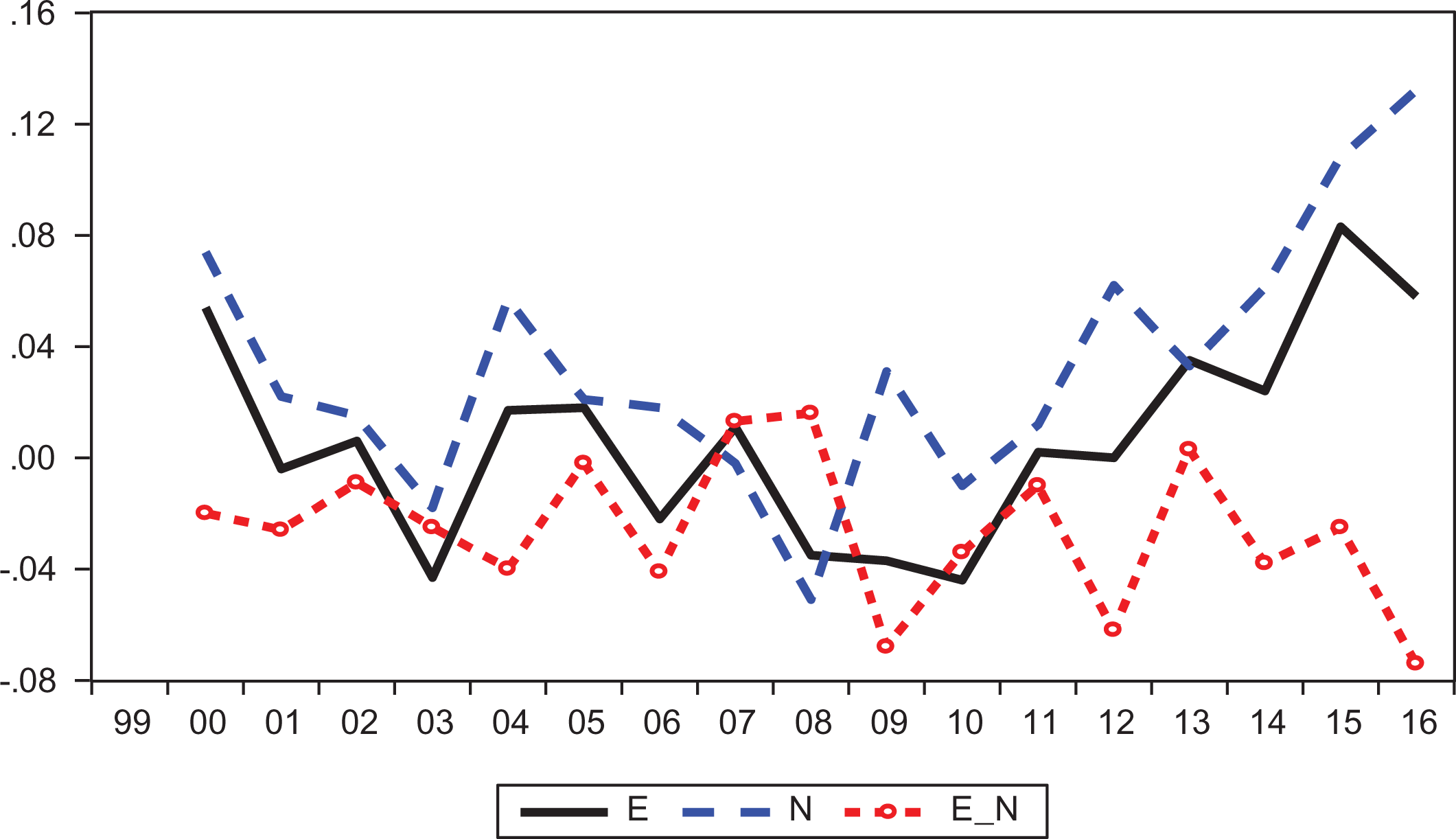
First differences of the annual fixed effects.

The trend in total tourist expenditures (E) and average expenditures (E/N) is more difficult to interpret due to the US$ effect. It should be noted that tourist expenditures are collected by the UNWTO in US$ to standardize the figures even though, at some destinations, neither the tourists nor the destination use this currency. Thus, fluctuations in the exchange rate between the US$ and other currencies could be responsible for some inter-annual changes. Hence, taking into account the potential bias that exchange rates might cause in the analysis, Table 3 shows that no significant differences have been reported in total tourist expenditures since 1998 (only 2016 is significantly higher than 1998, with a 10% difference).

To have a picture about how tourism flows, total expenditures and expenditures per capita have evolved during the last years unconditioned to the determining variables, Figure 1 represents the increase of the annual fixed effects. Then, first, it is shown how increases in total expenditures, despite the limitations in their interpretation mentioned above, have hovered close to 0%, with a positive trend during recent years. In the case of average tourist expenditures, the picture is different. From Table 3 and Figure 1, the period of our analysis clearly seems to be characterized by a negative trend. Consequently, despite the positive worldwide trend in tourist numbers, in recent years, international tourism flows seem to have been characterized by a drop in average expenditures.

Discussion

The results of the section on the empirical application show that the explanatory variables in the final demand models are consistent, suggesting that these variables have significant influences on tourism demand, whether it is measured through tourist arrivals, expenditure or average expenditure. Specifically, as theoretically argued, the main tourism determinants’ significant influence on average expenditure implies the existence of significant differences in the estimated parameters of the tourism demand equation, depending on whether the demand is measured in terms of tourist arrivals or total expenditure.

From the point of view of destination managers, although some of the determining variables are difficult to control, the results could be useful in predicting future trends. Thus, when the relationship between tourism demand and the level of development (measured in terms of the GDPpc) and the population at the destination were analysed, it was found that an increase in both the latter at a destination has a greater impact on tourist expenditure than on tourist arrivals. As for prices – a crucial determinant associated with some of the most recurrent controversial tourism policies, like taxes and currency exchange policies – interestingly the results show that higher prices are related to lower numbers of tourists and lower expenditures. However, it is important to highlight the fact that the effect on tourist arrivals is much greater than it is on tourist expenditures due to the positive effect of higher prices on average expenditures.

The results also show that the policy of increasing the length of the coastline, used by some countries during the last decades, could have limited effects on tourist expenditures despite the bigger effects on tourist arrivals. Other variables that destination managers can often influence are the promotion of new WHS and easier visa application procedures. In both cases, it was found that the effect on tourist arrivals is the opposite of the effect on average expenditures. Consequently, the effectiveness of these measures should be reconsidered when the objective is to increase the total revenue from tourism.

The annual fixed effects highlight the progressive growth of international tourist arrivals throughout the world during the last 18 years, with known interruptions brought about by the effects of 11-S and the financial crisis. However, despite the previously indicated methodological constraints, it seems that the general increase in tourist arrivals has not been transposed to tourist expenditures. The negative trend in average tourist expenditures appears to underlie this behaviour.

Conclusions

Tourism demand modelling seeks to reveal tourists’ economic reactions and preferences for trips to and/or from specific destinations. At an aggregate level, tourism demand has been measured through both tourist arrivals and tourist expenditures. From a theoretical point of view, there are substantial differences between the consideration of one or the other variable. However, different literature reviews have not distinguished this issue when analysing and quantifying the different tourism demand determinants, although they have found differences in the quantified reaction in terms of the demand elasticities depending on which variable was used.

This article has investigated the relationship between tourist arrivals and tourist expenditures within the framework of tourism demand at a destination level and the application of a regression analysis. The theoretical link between both measures in the context of a regression analysis has shown that the parameters of the two demand equations, measured in terms of tourist arrivals and tourist expenditure, may differ unless the determinants of the demand have no impact on average tourist expenditure. We found that the parameters of the demand equation, measured in terms of total expenditure, should be the sum of the parameters of the demand equation measured in terms of tourist arrivals and the parameters of a third demand equation that assesses average expenditure.

Given the empirical implications of the theoretical findings, this study estimated different tourism demand models at the destination level, considering international arrivals and tourist expenditures for 191 countries from 1998 to 2016. Our results show that when the tourist expenditure and arrival equations are compared, the elasticities and the rest of the equations’ parameters do not concur, although they are related through the estimated parameters of the third demand model that considers average expenditures. Thus, our findings shed some light on the differences in the estimated elasticities obtained in previous empirical literature.

From a practical point of view, our results are useful for defining tourism development strategies at destinations by pinpointing how determinants can affect tourist expenditures and tourism flows to differing extents. In this way, tourism destination managers will be more aware how different policies and different determinants can have a varying impact on tourist expenditures and tourist arrivals, deciding whether the objective is to maximize tourism flows or tourist expenditures. From the perspective of annual growth, we found that the progressive growth in international tourist arrivals in recent years has not gone hand-in-hand with an increase in tourist expenditures due to the negative trend shown in average tourist expenditures.

This article performs an in-depth analysis of differences in estimated parameters in tourism demand modelling, using the specific context of a destination-based tourism demand model. However, we could extend our results to other aggregate tourism demand models in other frameworks, such as time series analysis or gravity models. Future studies should be conducted to look further into the relationship between tourist expenditure and tourist arrival equations to provide additional evidence of our findings. In future applications of tourism-demand modelling, care should be taken in the measure that is chosen as the independent variable. Although a study’s specific objective or the availability of data can still be put forward as reasons for choosing tourist arrivals or tourist expenditures as the main variable, the results will be conditioned by the effect of the selected determinants on average expenditure.

Footnotes

Acknowledgements

We acknowledge the Agencia Estatal de Investigación (AEI) and the European Regional Development Funds (ERDF) for its support to the project <ECO2016-79124-C2-1-R> (AEI/ERDF, EU).

Declaration of conflicting interests

The author(s) declared no potential conflicts of interest with respect to the research, authorship, and/or publication of this article.

Funding

The author(s) disclosed receipt of the following financial support for the research, authorship, and/or publication of this article: Authors have received financial support from the Agencia Estatal de Investigación (AEI) and the European Regional Development Funds (ERDF) fthougth to the project (AEI/ERDF, EU).

References

Aguiló

Rosselló

Vila

(2017) Length of stay and daily tourist expenditure: a joint analysis. Tourism Management Perspectives 21: 10–17.

Anderson

van Wincoop

(2003) Gravity with gravitas: a solution to the border puzzle. American Economic Review 93: 170–192.

Brida

Scuderi

(2013) Determinants of tourist expenditure: a review of microeconometric models. Tourism Management Perspectives 6: 28–40.

Bujosa

Rosselló

(2013) Climate change and summer mass tourism: the case of Spanish domestic tourism. Climatic Change 117: 363–375.

Cho

(2001) Tourism forecasting and its relationship with leading economic indicators. Journal of Hospitality and Tourism 25: 399–420.

Crouch

(1994a) The study of international tourism demand: a survey of practice. Journal of Travel Research 32(4): 41–55.

Crouch

(1994b) The study of international tourism demand: a review of findings. Journal of Travel Research 33(1): 12–23.

Crouch

(1995) A meta-analysis of tourism demand. Annals of Tourism Research 22: 103–118.

Crouch

(1996) Demand elasticities in international marketing: a meta-analytical application to tourism. Journal of Business Research 36(2): 117–36.

10.

Crouch

Schultz

Valerio

(1992) Marketing international tourism to Australia: a regression analysis. Tourism Management 13: 196–208.

11.

De Haan

Lawrence

Litjens

(2018) Measurement error in dependent variables. Tilburg university Working Papers. Available at: https://www.tilburguniversity.edu/sites/tiu/files/download/Lawrence_2.pdf (accessed 28 June 2019).

12.

De Vita

Kyaw

(2013) Role of the exchange rate in tourism demand. Annals of Tourism Research 43: 624–627.

13.

Dogru

Sirakaya-Turk

Crouch

(2017) Remodeling international tourism demand: old theory and new evidence. Tourism Management 60: 47–55.

14.

Downward

Lumsdon

(2000) The demand for day-visits: an analysis of visitor spending. Tourism Economics 6: 251–261.

15.

Downward

Lumsdon

(2003) Beyond the demand for day-visits: an analysis of visitor spending. Tourism Economics 9: 67–76.

16.

Eymann

Ronning

(1997) Microeconometric models of tourists’ destination choice. Regional Science and Urban Economics 27(6): 735–761.

17.

Fleischer

Rivlin

(2009) More or better? Quantity and quality issues in tourism consumption. Journal of Travel Research 47: 285–294.

18.

Fourie

Santana-Gallego

(2011) The impact of mega-sport events on tourist arrivals. Tourism Management 32: 1364–1370.

19.

Fourie

Santana-Gallego

(2013) Ethnic reunion and cultural affinity. Tourism Management 36: 411–420.

20.

Fourie

Rosselló-Nadal

Santana-Gallego

(2020) Fatal attraction: how security threats hurt tourism. Journal of Travel Research 59(2): 209–219.

21.

Hamilton

Maddison

Tol

RSJ

(2005) The effects on climate change on international tourism. Climate Research 29: 245–254.

22.

Hamilton

Tol

RSJ

(2007) The impact of climate change on tourism in Germany, the UK and Ireland: a simulation study. Regional Environmental Change 7: 161–172.

23.

Kandogan

(2008) Consistent estimates of regional blocs, trade effects. Review of International Economics 162: 301–314.

24.

Khadaroo

Seetanah

(2008) The role of transport infrastructure in international tourism development: a gravity model approach. Tourism Management 29: 831–840.

25.

Kulendran

Divisekera

(2007) Measuring the economic impact of Australian tourism marketing expenditure. Tourism Economics 13: 26–274.

26.

Lim

(1997a) An econometric classification and review of international tourism demand models. Tourism Economics 3: 69–81.

27.

Lim

(1997b) Review of international tourism demand models. Annals of Tourism Research 24(4): 835–849.

28.

Lim

(1999) A meta-analytic review of international tourism demand. Journal of Travel Research 37(3): 273–284.

29.

Lyons

Mayor

Tol

RSJ

(2009) Holiday destinations: understanding the travel choices of Irish tourists. Tourism Management 30: 683–692.

30.

McConnell

(1992) On-site time in the demand for recreation. American Journal of Agricultural Economics 74: 918–925.

31.

Morley

(1992) A microeconomic theory of international tourism demand. Annals of Tourism Research 19: 250–267.

32.

Morley

(1995) Tourism demand: characteristics, segmentation and aggregation. Tourism Economics 1: 315–328.

33.

Morley

(1998) A dynamic international demand model. Annals of Tourism Research 25: 70–84.

34.

Morley

Rosselló

Santana-Gallego

(2014) Gravity models for tourism demand: theory and use. Annals of Tourism Research 48: 1–10.

35.

Neumayer

(2010) Visa restrictions and bilateral travel. The Professional Geographer 62: 171–181.

36.

Ditton

(2005) An evaluation of price measures in tourism demand models. Tourism Analysis 10: 257–268.

37.

Papatheodorou

(2001) Why people travel to different places. Annals of Tourism Research 28: 164–179.

38.

Peng

Song

Crouch

(2014) A meta-analysis of international tourism demand forecasting and implications for practice. Tourism Management 45: 181–193.

39.

Peng

Song

Crouch

, et al. (2015) A meta-analysis of international tourism demand elasticities. Journal of Travel Research 54(5): 611–633.

40.

Qiu

Zhang

(1995) Determinants of tourist arrivals and expenditures in canada. Journal of Travel Research 34(2): 43–49.

41.

Rosselló

(2015) Elasticity, demand and supply in tourism. In: Jafari

Xiao

(eds) Encyclopedia of Tourism. Switzerland: Springer. DOI: 10.1007/978-3-319-01669-6_67-1.

42.

Rosselló

Santana-Gallego

(2014) Recent trends in international tourist climate preferences: a revised picture for climatic change scenarios. Climatic Change 124(1–2): 119–132.

43.

Rosselló

Santana-Gallego

Waqas

(2017) Infectious disease risk and international tourism demand. Health Policy and Planning 32(4): 538–548.

44.

Rosselló-Nadal

Riera-Font

Cárdenas

(2011) The impact of weather variability on British outbound flows. Climatic Change 105: 281–292.

45.

Santana-Gallego

Fourie

Rosselló

(2019) The effect of safety and security issues on international tourism. Annals of Tourism Research. Epub ahead of print February 2019. DOI: 10.1016/j.annals.2019.02.004.

46.

Santeramo

Morelli

(2016) Modelling tourism flows through gravity models: a quantile regression approach. Current Issues in Tourism 19: 1077–1083.

47.

Seddighi

Theocharous

(2002) A model of tourism destination choice: a theoretical and empirical analysis. Tourism Management 23: 475–487.

48.

Seetaram

Dwyer

(2009) Immigration and tourism demand in Australia: a panel data analysis. Anatolia 20: 212–222.

49.

Sheldon

(1993) Forecasting tourism: expenditures versus arrivals. Journal of Travel Research 32(1): 13–20.

50.

Smeral

(1988) Tourism demand, economic theory and econometrics: an integrated approach. Journal of Travel Research 26(4): 38–43.

51.

Smeral

(2008) The impact of the financial and economic crisis on european tourism. Journal of Travel Research 48(1): 3–13.

52.

Song

(2008) Tourism demand modelling and forecasting - A review of Recent research. Tourism Management 29: 203–220.

53.

Song

Witt

, et al. (2010) Tourism demand modelling and forecasting: how should demand be measured? Tourism Economics 16(1): 63–81.

54.

Song

Witt

(2009) The Advanced Econometrics of Tourism Demand. New York: Routledge.

55.

Song

Wong

KKF

(2003) Tourism demand modelling: a time-varying parameter approach. Journal of Travel Research 42: 57–64.

56.

Thrane

(2008) The determinants of students’ destination choice for their summer vacation trip. Scandinavian Journal of Hospitality and Tourism 8: 333–348.

57.

Turner

Witt

(2001) Factors influencing demand for international tourism: tourism demand analysis using structural equation modeling, revisited. Tourism Economics 7: 21–38.

58.

Varian

(2010) Intermediate Microeconomics. A Modern Approach, 8th ed. New York; London: WW Norton & Company.

59.

Witt

(1995) Forecasting tourism demand: a review of empirical research. International Journal of Forecasting 11(3): 447–475.