Tourism forecast combination using the stochastic frontier analysis technique

Abstract

Forecast combination has received a great deal of attention in the tourism domain. In this article, we propose a novel performance-based tourism forecast combination model by applying a multiple-criteria decision-making framework and the stochastic frontier analysis technique to determine combination weights for individual tourism forecast models. Thirteen time-series models are used to generate individual forecast tourism models, and five competing forecast combination models are selected to evaluate the forecast performance. Using the tourism forecast competition data set, we conclude that the proposed combination model significantly and statistically outperforms the five competing combination models in most cases based on multiple performance indicators. Our results show that the proposed model offers a good solution to identify optimal weights for individual tourism forecast models.

Keywords

forecast combination SFA time-series model tourism forecasting

Introduction

The tourism industry contributes significantly to global economic growth and recovery, as it benefits a number of related service industries, such as transportation, retail, catering and hotels (Liu et al., 2018; Sun et al., 2019). According to a recent report from the Ministry of Culture and Tourism of the People’s Republic of China, in 2018, the total tourism revenue in China was USD870 billion, an increase of 10.8% over the previous year, accounting for 11.04% of China’s total GDP.¹ Correspondingly, tourism forecasting has received widespread attention from researchers and practitioners. Accurate tourism forecasting not only improves the ability of tourism firms to make decisions, such as in creating budget plans, making hotel investments and managing human resources, but it also helps governments make appropriate tourism policies in, for example, residential site planning, tourism marketing strategies and transportation system design (Jiao and Chen, 2018; Li et al., 2018).

Studies on tourism forecasting have continued to receive much attention in academic research. In a recent literature review of 171 papers published in 2007–2015, Wu et al. (2017) found that the most commonly used approaches in tourism forecasting can be classified into three categories: non-causal time-series methods, causal econometric methods and artificial intelligence methods. Although many tourism forecast models have been proposed in the literature, most researchers mainly use single forecast models to obtain the best forecasting performance. However, there is no universal single forecast model that outperforms others in all situations (Cang and Yu, 2014; Shen et al., 2011). Furthermore, empirical research in other fields has already shown that forecast combination modelling significantly improves forecast accuracy and often produces better results than the best individual forecast model (Cang and Yu, 2014; Timmermann, 2006). Although the idea of tourism forecast combination has received increasing attention in academia, it is still considered a new development in tourism forecasting (Wu et al., 2017). Since 2007, there have been several papers on tourism forecast combination. Table 1 shows a brief review of this literature.

Table 1.

An overview of selected tourism forecast combination literatures.

References	Region focused	Research objects	Data frequency	Combination method	No. of individual model
Cang and Yu (2014)	UK	Inbound tourism	Quarterly	SA, VACO, DMSFE	Nine individual models
Shen et al. (2011)	UK	Outbound tourism	Quarterly	SA, VACO, DMSFE, GR, shrinkage, TVP	Five individual models
Coshall and Charlesworth (2011)	UK	Outbound tourism	Quarterly	SA, VACO, Goal combination	Four individual models
Chen (2011)	Taiwanese	Outbound tourism	Monthly	Decomposition	Five individual models
Cang (2011)	UK	Inbound tourism	Quarterly	SA, VACO, DMSFE, LMPNN	Nine individual models
Andrawis et al. (2011)	Egypt	Inbound tourism	Monthly	SA, VACO, INV-MSE, IRANK, etc.	Two individual models
Chan et al. (2010)	Hong Kong	Inbound tourism	Quarterly	SA, VACO, CUSUM	Four individual models
Song et al. (2009)	Hong Kong	Inbound tourism	Quarterly	SA, VACO, DMSFE	Four individual models
Shen et al. (2008)	UK	Outbound tourism	Quarterly	SA, VACO, DMSFE	Seven individual models
Wong et al. (2007)	Hong Kong	Inbound tourism	Quarterly	SA, VACO, DMSFE	Four individual models

Tourism forecast combination is achieved by assigning weights to individual forecast models. The combination method used in tourism forecasting can be generalized as two weight generation schemes: the simple average (SA) and the optimal weight (OW) technique. The SA approach assigns constant weights to individual models, whereas the OW methods assign weights based on a function of forecast error-derived accuracy measures, which are used to evaluate the forecasting performance of an individual model. For example, one widely used OW technique is the variance–covariance combination (VACO) method (Cang and Yu, 2014). In VACO, the weights are proportional to the performance of the individual forecast models, with the performance of the individual models evaluated solely by mean square error (MSE). It may be unreliable to evaluate the performance of individual tourism forecast models based only on one accuracy measure, as there exist various accuracy measures, such as mean absolute error (MAE), mean absolute percentage error (MAPE) and others. Different accuracy measures have different advantages and disadvantages. Hyndman and Koehler (2006) conducted a comprehensive review of the accuracy measures used in the forecasting field and presented an exhaustive discussion of their advantages and disadvantages. For example, in the article, the authors concluded that the root mean square error (RMSE) and MSE are more sensitive to outliers than MAE, and that the measures based on percentage error (e.g. MAPE) are often highly skewed. Under this consideration, the results of performance evaluations for individual forecast models will vary depending on the accuracy measures used. In fact, studies from empirical forecast competitions, such as the M competition (Makridakis et al., 1982), the M3 competition (Makridakis and Hibon, 2000) and the NN3 competition (Crone et al., 2011), have found that the performance of forecast models varies considerably depending on the selected accuracy measures. Thus, we question why multiple accuracy measures are not used to determine the combination weight for individual tourism forecast models.

In this study, we argue that the performance evaluation results of individual tourism forecast models can be more reliable and robust by considering multiple accuracy measures, and we propose a novel performance-based combination model for tourism forecasting. Specifically, we consider the problem of performance evaluation for individual forecast models with multiple accuracy measures as a classic multiple-criteria decision-making (MCDM) problem, and we use the stochastic frontier analysis (SFA) technique to solve this MCDM problem. In other words, we use SFA to calculate the combination weight of individual forecast models based on their forecasting performance, which is denoted by the technique efficiency value obtained by SFA. To illustrate the effectiveness of the performance-based combination model, we adopt four widely used accuracy measures in our case study, RMSE, MAE, MAPE and mean absolute scaled error (MASE), to assign weights for 13 individual tourism forecast models. This illustration uses the renowned tourism forecast competition data set (Athanasopoulos et al., 2011) and is compared with five linear combination models. The tourism forecast competition data set contains 1311 tourism time series with different time intervals, including 518 yearly series, 427 quarterly series and 366 monthly series. The results show that the performance-based combination model significantly and statistically outperforms the five competing combination models in most cases based on the multiple performance indicators used.

This study offers several contributions. First, our article extends the tourism forecast combination literature by proposing a novel combination method in which the combination weight is generated based on a MCDM framework and the SFA technique. Our study extends the traditional work of tourism forecast combination research studies, such as Wong et al. (2007), Chan et al. (2010), Shen et al. (2011) and Cang and Yu (2014), which calculate the weights solely on one accuracy measure function (e.g. VACO). Second, our article offers a comprehensive comparison among forecast combination techniques, unlike traditional comparison studies that usually use one accuracy measure and combine two individual tourism forecast models (e.g., Chen, 2011). In this article, we consider 13 individual tourism forecast models and 5 forecast combination models. Furthermore, to give a comprehensive comparison, we use the tourism forecast competition data set, which contains 1311 tourism time-series data.

The article is organized as follows. The second section presents the related theories. The third section describes the model-building process. The fourth section demonstrates the experimental process and analyses the results. The fifth section reports our conclusions and discusses our findings.

Related works

Forecasting studies

Forecasting is concerned with the prediction of future values based on historical data and has extensive applications in a variety of topics in the business research domain, such as supply chain forecasting (Svetunkov and Boylan, 2019), order management (Van Gils et al., 2017), demand forecasting (Prestwich et al., 2014) and finance forecasting (Podsiadlo and Rybinski, 2016). Traditionally, forecasting studies have used statistical models, such as exponential smoothing (Petropoulos et al., 2018), autoregressive integrated moving average (ARIMA) (Azevedo and Campos, 2016) and the TBATS model (De Livera et al., 2011). Machine learning techniques, such as the neural network model (dos Santos and Vellasco, 2015), the support vector machine (Chen and Lee, 2015) and the k-nearest neighbour model (Cai et al., 2016), have also drawn a great deal of attention in the forecasting field. In these models, researchers identify the best single statistical model for prediction. Recently, there has been a transition from individual deterministic forecast to forecast combination. Forecast combination linearly integrates several individual models and has widely proved to be a highly successful forecasting strategy (Adhikari, 2015; Podsiadlo and Rybinski, 2016), as it significantly improves forecasting accuracy and often produces better results than the best individual forecast model (Cang and Yu, 2014; Timmermann, 2006).

As tourism planning and administration rely on efficient and accurate forecast techniques (Hirashima et al., 2017; Turner and Witt, 2001), tourism forecasting has become a relevant research field. A decision maker can choose from among several tourism forecast models. Deserted models might still have some useful information, and thus a combination strategy that incorporates several individual models might provide better accuracy. Combination strategy originated in the 1960s with the work of Bates and Granger (1969), and since then, it has been studied extensively in the forecasting domain. Indeed, it has been shown that combining several individual tourism forecast models can lead to superior performance in accuracy (Cang, 2011). Wong et al. (2007) first conducted a comprehensive investigation for three forecast combination strategies: SA, VACO and discounted mean square forecast error (DMSFE). They concluded that the combination strategies improve forecast accuracy, although such strategies might not always be better than the best individual forecast model in all situations. Following the research framework of Wong et al. (2007) and Shen et al. (2008), Song et al. (2009) further assessed tourism forecast combination. By carrying out comparisons among the same three combination strategies and individual forecast models, they found that combined forecasts are more accurate than individual tourism forecast models. Table 1 lists several tourism forecast combination studies since 2007.

From Table 1, we see that the tourism forecast combination technique can be generalized into two weight generation schemes: the SA and the OW methods. The SA technique assigns constant weights for individual models, whereas in the OW techniques, the weights are a function of forecast error derived from accuracy measures. For example, in the VACO method, the weight for each individual forecast is a function of the MSE with the aim of minimizing the in-sample error variance; in the DMSFE method, the weight is related to MSE, but it incorporates the discount factor. There are also several variations of the VACO method: the inverse of the mean square error (INV-MSE) method (Andrawis et al., 2011), the inverse of performance rank (IRANK) method (Andrawis et al., 2011) and the cumulative sum (CUSUM) method (Chan et al., 2010). There are also several regression models, such as ordinary least squares and constrained least squares (Andrawis et al., 2011) and the ridge regression method (Chan et al., 1999). However, the regression framework has proved to perform poorly in many cases (Sermpinis et al., 2012).

Despite the large number of combination approaches available, there is no unanimity on the best weighting approach in general empirical situations. One major reason might be that the combination weight for individual models relies solely on one accuracy measure, and the performance evaluation result for individual models might be different depending on the accuracy measure used.

Accuracy measures

To evaluate the performance of forecasting models, a large number of accuracy measures have been proposed in academic research including but not limited to the tourism field. However, such accuracy measures are bewildering and not generally applicable as different accuracy measures evaluate different types of forecast error and can produce misleading results. Hyndman and Koehler (2006) conducted a comprehensive examination on accuracy measures and classified these measures into four groups: scale-dependent measures, percentage error-based measures, relative error-based measures and relative measures. We briefly present these measures here.

Forecast error is defined as $e_{t} = Y_{t} - F_{t}$ , where Y_t denotes the observation at time t, and F_t denotes the forecast of Y_t . The first category of accuracy measures is scale-dependent measures, which include MAE, median absolute error (MdAE), MSE and RMSE. The scale-dependent measure is appropriate for comparing different forecast methods used to the same time-series data, but they might not be suitable for heterogeneous time series. The second category is percentage error measures in which the percentage error is obtained based on $P_{t} = 100 e_{t} / Y_{t}$ . Percentage error measures include MAPE, median absolute percentage error (MdAPE), root mean square percentage error (RMSPE) and root median square percentage error (RMdSPE). This measure also has shortcomings, such as the percentage error measure being infinite, having a skewed distribution if Y_t equals or is close to zero or being undefined if $Y_{t} = F_{t} = 0$ . The third category is relative error-based measures, which are calculated by dividing the forecast error by the error of the benchmark forecast model. There are three common measures in this category: mean relative absolute error (MRAE), median relative absolute error (MdRAE) and geometric mean relative absolute error (GMRAE). It is important to select a suitable benchmark model for calculating the relative error measure. The fourth category is relative measures, which are similar to relative error-based measures. Take, for example, relative MAE, which can be defined as $Rel_MAE = {MAE/MAE}_{b}$ , where ${MAE}_{b}$ is the MAE of the benchmark forecast model. One disadvantage of relative error-based measures and relative measures is that they cannot be calculated in a straightforward manner over various data because the measures rely on the relative errors. Another disadvantage is that they might lead to unexpected or undesired measures as a result of the choice of benchmark model.

The choice of appropriate accuracy measures to evaluate the performance of forecast methods is a topic of interest in the forecasting field. However, the choice of suitable accuracy measures remains controversial (Davydenko and Fildes, 2013). Here we illustrate the controversy with several examples: (i) In the original M competition, MAE was always used by Makridakis et al. (1982). However, as Armstrong and Collopy (1992) pointed out, MAE is not suitable for different time-series data. Armstrong (2001) also recommended against the use of RMSE in forecast accuracy evaluation even though RMSE has been popular in much of the literature because RMSE is more sensitive to outliers as compared to MAE or MdAE. Instead, Armstrong and Collopy (1992) suggested the choice of relative absolute errors. (ii) In the M3 competition, Makridakis and Hibon (2000) suggested MdRAE, sMAPE and sMdAPE. However, Swanson et al. (2000) and Coleman and Swanson (2007) showed that accuracy measures based on percentage measures have highly skewed distribution. (iii) MASE, which can overcome the shortcomings of percentage measures, was recommended by Hyndman and Koehler (2006). However, MASE has disadvantages. For example, MASE has a bias towards overestimating the benchmark model, and it is vulnerable to outliers (Davydenko and Fildes, 2013).

We conclude that many of the accuracy measures are not generally applicable. That is, although such measures have been used to evaluate forecast performance, all of them have shortcomings. Different accuracy measures can result in different performance outcomes. Makridakis and Hibon (2000) pointed out that the relative ranking of the performance of forecast models varies when different accuracy measures are chosen. Crone et al. (2011) had similar results from their NN3 competition research. As such, forecasting performance evaluation cannot obtain consistent results, as different accuracy measures might produce different results. We argue that it might be more reliable and robust to evaluate forecast performance by considering multiple accuracy measures so that these accuracy measures complement each other and take into account more information from individual forecast models. In this way, performance evaluation based on multiple accuracy measures can provide a more robust and convincing result, and thus the combination weight obtained from this performance evaluation result will also be more robust.

The performance-based combination model

The performance-based combination framework

There are three types of tourism forecasting methods: (i) non-causal time-series methods (Hassani et al. 2017), (ii) causal econometric methods (Wan and Song, 2018) and (iii) artificial intelligence methods (Li et al. 2018). In this article, we mainly focus on non-causal time-series methods, which involve the using of historical tourism data to predict the future.

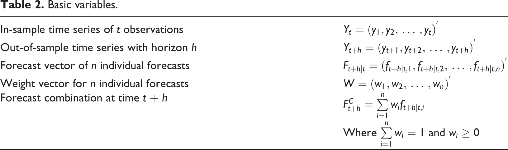
First, in Table 2, we define the variables used in this article. We divide the tourism time-series data into two parts: the in-sample series of first t observations are used to train a forecast model, and the out-of-sample series of the last h observations are used to test the forecast model. If there are n individual forecast models, we can obtain a forecast vector that contains n forecast values for the out-of-sample series. The major challenge of tourism forecast combination is to assign weights for each individual forecast model based on a suitable weight generation scheme.

Table 2.

Basic variables.

In-sample time series of t observations	$Y_{t} = {(y_{1}, y_{2}, \dots, y_{t})}^{'}$
Out-of-sample time series with horizon h	$Y_{t + h} = {(y_{t + 1}, y_{t + 2}, \dots, y_{t + h})}^{'}$
Forecast vector of n individual forecasts	$F_{t + h \| t} = {(f_{t + h \| t, 1}, f_{t + h \| t, 2}, \dots, f_{t + h \| t, n})}^{'}$
Weight vector for n individual forecasts	$W = {(w_{1}, w_{2}, \dots, w_{n})}^{'}$
Forecast combination at time t + h	$F_{t + h}^{C} = \sum_{i = 1}^{n} w_{i} f_{t + h \| t, i}$ Where $\sum_{i = 1}^{n} w_{i} = 1$ and $w_{i} \geq 0$

As mentioned above, there are two major motivations: one is that the combination weight estimated solely upon one accuracy measure is not reliable and robust because it amplifies the variance of the combination and leads to biased results; the other is that the performance evaluation results for individual forecasts are different based on different accuracy measures as different measures evaluate different aspects of the forecast error. Therefore, we propose a novel performance-based combination model. Specifically, we first evaluate the performance of each individual forecast model by taking into account multiple accuracy measures. We consider such performance evaluation under multiple accuracy measures as a classic MCDM problem, succinctly defined as making decisions involving multiple attributes/objectives (Zionts, 1992). Then we obtain the performance value (PV) for each individual forecast model by solving the MCDM problem. Lastly, we calculate the weight for each individual model based on the proportion of its PV to the sum of all of the models. The upper part of Figure 1 shows the MCDM framework.

Figure 1.

Performance-based forecast combination framework.

In the classic MCDM methodology, it is assumed that there are many alternatives and each alternative is measured by its value on each of the multiple attributes (Stewart, 1996). A decision maker must decide which alternatives are best and sort the alternatives. The MCDM methodology supports decision makers in evaluating the performance of the alternatives. In this article, the performance-based combination method is precisely in line with the MCDM methodology, in which the alternatives are the individual tourism forecast models and the attributes correspond to the multiple accuracy measures. In particular, we can obtain k accuracy measures, denoted as ( ${AM}_{1}, {AM}_{2}, \dots, {AM}_{k}$ ), for each individual forecast model based on the out-of-sample series. These accuracy measures are considered as the performance attributes, and the n individual forecast models are viewed as the alternatives. In the MCDM methodology, we need to calculate a PV for each individual model.

Here we use SFA to solve the MCDM problem. The PV of an individual forecast model can be measured by its technical efficiency value (TEV), and the TEV can be estimated by SFA. SFA is a parametric approach for benchmarking and has been developed simultaneously by Meeusen and van den Broeck (1977) and Aigner et al. (1977). SFA has several advantages: first, in SFA, the production function that shows the relationship between the input and output is supposed to be known and can be estimated statistically (Hailu and Tanaka, 2015); second, the error term integrates the stochastic component and the non-negative inefficiency component (Anaya and Pollitt, 2017); third, the hypothesis for SFA is statistically rigorous and can be theoretically tested, and the technical inefficiency effects model and the stochastic production model can be simultaneously estimated for the SFA technique (Charoenrat and Harvie, 2014).

Consider a set of n individual tourism forecast models, with each model j (j = 1,…, n), using k − 1 inputs $a m_{i j}$ (i = 1,…, k − 1) and generating one output ${\bar{a m}}_{k j}$ . Specifically, k − 1 inputs and a one-output Cobb–Douglas production function can be expressed as follows:

\begin{matrix} ln ({\bar{a m}}_{k j}) = β_{0} + \sum_{i = 1}^{k - 1} β_{i} ln (a m_{i j}) + v_{j} - u_{j} \\ j = 1, 2, \dots, n \end{matrix}

where ${\bar{a m}}_{k j}$ is the reciprocal of $a m_{k j}$ and is considered as the output for individual model j. The random error term $v_{j} \sim i i d (0, σ_{v}^{2})$ and the inefficiency component $u_{j} \sim i i d (μ, σ_{u}^{2})$ are supposed to be random and independent from frontier regressors and v_j . By estimating equation (1), the inefficiency estimates ${\hat{u}}_{j}$ can be obtained from the residuals as ${\hat{u}}_{j} = max {{\hat{u}}_{j}^{*}} - {\hat{u}}_{j}^{*}$ .

It is worth highlighting that u_j denotes the ‘inefficiency’ term. To estimate the TEV for each individual forecast model, we transform the ‘inefficiency’ term into the ‘efficiency’ term with equation (2), as discussed in detail by, for example, Kumbhakar and Lovell (2003).

{TEV}_{j} = exp [- {\hat{u}}_{j}]

As the PV of an individual forecast model is measured by TEV, the weight w_j for individual forecast model j can be calculated based on equation (3):

w_{j} = {PV}_{j} / \sum_{i = 1}^{n} {PV}_{i} = {TEV}_{j} / \sum_{i = 1}^{n} {TEV}_{i}

Competing forecast combination and individual tourism forecast models

In the proposed performance-based forecast combination, the weights are based on the PVs obtained by the SFA technique, which considers multiple accuracy measures. In the rest of the article, we refer to the proposed performance-based forecast combination as the SFA-based model. We use five different combination models in our tourism forecast combination model comparison: three, namely equal weight (EW), trimmed mean (TM) and Winsorized mean (WM), belong to the SA category, and the other two, the VACO model (Bates and Granger, 1969) and the IRANK model (Aiolfi and Timmermann, 2006), belong to the OW category. A summary description of the competing forecast combination models is provided in Table 3. In particular, the EW model, which simply assigns equal combination weights for all individual forecast models, is widely used and often considered as a benchmark combination approach in much of the forecast literature. The TM and WM weighting models are two variations of the EW model but are quite robust compared to the EW model. Trimming is the removal of extreme values, and winsorizing is reducing the outermost values in extremity. The VACO model is a classic OW method in which the weight generating is based on one accuracy measure, MSE. The IRANK model is a variant of the VACO model that considers the ranking order of the individual models. It is worth highlighting that there are many variants of VACO. In this article, we use the RANK model as a representative.

Table 3.

Summary description of the tourism forecast models.

Forecast model		Description	Code
Competing tourism forecast combination
SA	Equal weight	$F_{EW}^{C} = \frac{1}{n} \sum_{i = 1}^{n} f_{t + h \| t, i}$	EW
	Trimmed mean	$F_{TM}^{C} = \frac{1}{n (1 - 2 λ)} \sum_{i = λ n + 1}^{(1 - λ) n} f_{t + h \| t, i}$ , where the top/bottom λ% are trimmed based on RMSE	TM
	Winsorized mean	$F_{WM}^{C} = \frac{1}{n} [k f_{t + h \| t, (k + 1)} + \sum_{i = k + 1}^{n - k} f_{t + h \| t, i} + k f_{t + h \| t, (n - k)}]$ , where $k = n λ$ , λ is a trim factor: the top/bottom λ% are Winsorized based on RMASE	WM
OW	Bates–Granger model	$F_{VACO}^{C} = \sum_{i = 1}^{n} w_{i} f_{t + h \| t, i}$ , where $w_{i} = {MSE}_{i}^{- 1} / \sum_{j = 1}^{n} {MSE}_{j}^{- 1}$	VACO
OW	Inverse rank model	$F_{IRANK}^{C} = \sum_{i = 1}^{n} w_{i} f_{t + h \| t, i},$ where $w_{i} = {Rank}_{i}^{- 1} / \sum_{j = 1}^{n} {Rank}_{j}^{- 1}$	IRANK
Individual tourism forecast models
Exponential smoothing	Simple exponential smoothing model	$F_{t + h \| t} = ℓ_{t}$ ; $ℓ_{t} = α y_{t} + (1 - α) ℓ_{t - 1}$ . where α is the smoothing parameter for the level	SES
	Holt’s linear trend model	$F_{t + h \| t} = ℓ_{t} + h b_{t}$ ; $ℓ_{t} = a y_{t} + (1 - a) (ℓ_{t - 1} + b_{t - 1})$ ; $b_{t} = β (ℓ_{t} - ℓ_{t - 1}) + (1 - β) b_{t - 1}$ , where β is the smoothing parameter for the trend	Holt1
	Holt’s damped trend model	$F_{t + h \| t} = ℓ_{t} + (\emptyset + \emptyset^{2} + ... + \emptyset^{h}) b_{t}$ ; $ℓ_{t} = a y_{t} + (1 - a) (ℓ_{t - 1} + \emptyset b_{t - 1})$ ; $b_{t} = β (ℓ_{t} - ℓ_{t - 1}) + (1 - β) \emptyset b_{t - 1}$ , where ∅ is the damping parameter	Holt2
	Holt–Winters’ additive model	$F_{t + h \| t} = ℓ_{t} + h b_{t} + s_{t + h - m (k + 1)}$ ; $ℓ_{t} = a (y_{t} - s_{t - m}) + (1 - a) (ℓ_{t - 1} + b_{t - 1})$ ; $b_{t} = β (ℓ_{t} - ℓ_{t - 1}) + (1 - β) b_{t - 1}$ ; $s_{t} = γ (y_{t} - ℓ_{t - 1} - b_{t - 1}) + (1 - γ) s_{t - m}$	HW
	ARIMA model	$F_{t + h \| t} = μ + β_{1} y_{t - 1} + β_{2} y_{t - 2} + \dots + β_{p} y_{t - p} + θ_{1} ε_{t - 1} + θ_{2} ε_{t - 2} + \dots + θ_{p} ε_{t - p} + ε_{t}$	ARMA
Complex methods	BATS model	Refers to De Livera et al. (2011)	BATS
	TBATS model	Refers to De Livera et al. (2011)	TBATS
	Croston model	Refers to Shenstone and Hyndman (2005)	CRO
	Cubic spline model	Refers to Hyndman et al. (2005)	SPL
	Theta model	Refers to Assimakopoulos and Nikolopoulos (2000)	Theta
Simple methods	Mean model	$F_{t + h \| t} = (y_{1} + y_{2} + \dots + y_{t}) / t$	Meanf
	Naïve model	$F_{t + h \| t} = y_{t}$ .	RWF1
	Drift model	$F_{t + h \| t} = y_{t} + \frac{h}{t - 1} \sum_{i = 2}^{t} (y_{t} - y_{t - 1})$	RWF2

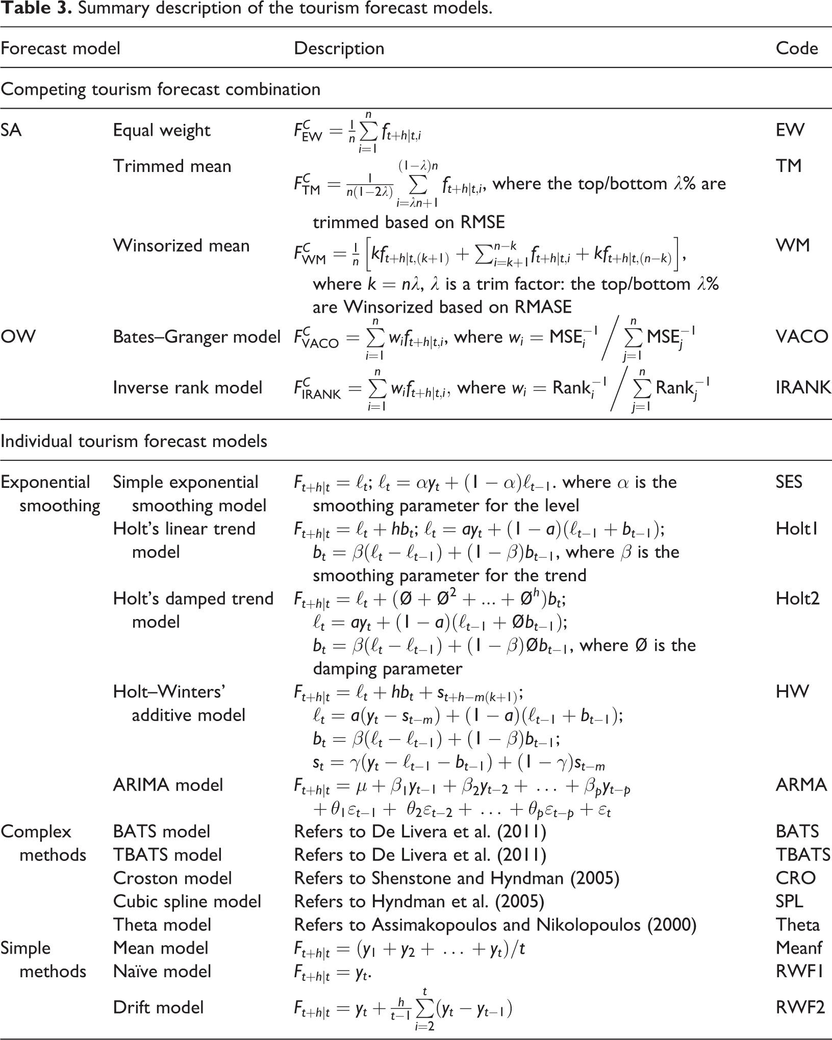
In this case study, 13 individual forecast models are built to form the forecast combination. A summary description of the individual forecast models is provided in Table 3. These individual models can be classified into four categories: exponential smoothing, ARIMA, complex methods and simple methods. Among these models are the most popular forecast methods, such as Holt’s linear trend model, Holt–Winters’ additive method and the ARIMA model. We also use five complex models that are newly emerging techniques – the BATS model, TBATS model, Croston model, cubic spline model and theta model – along with three simple methods, the mean model, naïve model and drift model, which are usually viewed as benchmark models in much of the time-series forecast literature.

Empirical investigation and analysis

Data sets and experimental design

In this study, to empirically compare the proposed performance-based tourism forecast combination model to the five competing combination models presented in ‘The Performance-based Combination Model’ section, we use the tourism data from the renowned tourism forecast competition data set (Athanasopoulos et al., 2011). The data set is available in the ‘Tcomp’ package in CRAN (https://cran.r-project.org) and contains 518 yearly series, 427 quarterly series and 366 monthly series. These data were supplied by various academics and several tourism bodies, such as Tourism New Zealand, the Hong Kong Tourism Board and Tourism Australia (Athanasopoulos et al., 2011). Table 4 reports in more detail the number of series and the length, frequency and forecast horizon for each frequency. The forecast horizon is also the length of the out-of-sample test data for each frequency in this study. Because of its diversification of data type, the tourism forecast competition data set has become an important data set for comparing alternative tourism forecast models.

Table 4.

Descriptive statistics of the tourism forecast competition data set.

Frequency		Monthly	Quarterly	Yearly
Number of series		366	427	518
Length
Mean	298.6	99.6	24.5
Median	330.0	110.0	27.0
Min	91.0	30.0	11.0
Max	333.0	130.0	47.0
Horizon		24	8	4

As mentioned, the performance-based combination model is a classic MCDM problem. To realize the MCDM framework, we use the four accuracy measures of RMSE, MAE, MAPE and MASE to form the attributes in this framework as these measures are often used to compare tourism forecast models. For the SFA model, the inputs are RMSE, MAE and MAPE for each individual forecast model, and the output is the reciprocal of MASE. Thus, in the SFA framework, there are 13 individual forecast models, and each individual forecast model has three inputs and one output. The major processes in the experiment are described as follows.

Step 1: Preparing the data. For each time series in the tourism forecast competition data set, we divided it into two parts: the in-sample series for training the forecast model and the out-of-sample series for testing the model. The length of the out-of-sample data set for each series with a different frequency is consistent with its corresponding forecast horizon. The lengths of the out-of-sample data set for the monthly, quarterly and yearly series are 24, 8 and 4, respectively.

Step 2: Training the individual tourism forecast models. For each time series, we use the in-sample data set to train the 13 individual forecast models. We check the collinearity of these models.

Step 3: Computing inputs and outputs for each individual forecast model. In this case, we calculate RMSE, MAE, MAPE and MASE for each individual forecast model based on the in-sample data set for each series. We set RMSE, MAE and MAPE as the inputs and the reciprocal of MASE as the output.

Step 4: Combining the individual forecast models. We combine the individual forecast models into the proposed performance-based combination model and the five competing combination models.

Step 5: Comparing the forecast combination models. We compare the performance of the six forecast combination models based on the out-of-sample data set by using multiple performance indicators.

As mentioned in ‘Accuracy measures’ section, different accuracy measures may yield different results in validating the performance of the forecast model. Therefore, in this article, we introduce several performance indicators to identify the ‘effectiveness’ of the SFA combination model. As there are six forecast combination models and many time-series data, we use three relative accuracy measures: relative RMSE (Rel_RMSE), relative MAE (Rel_MAE) and relative MAPE (Rel_MAPE). The relative RMSE is the RMSE of a certain forecast combination model in relation to the RMSE of the baseline forecast. We set the best individual forecast model as the baseline forecast, although the best individual forecast model might be different for different accuracy measures or different time series. We also present the mean rank of each forecast combination model. Considering time series i, we rank the six forecast combination models based on the selected relative accuracy measure (i.e. Rel_RMSE) with the best model being ranked as one and the worst as six. The mean rank of one forecast combination model is thus the average of the rankings of the target combination model over all of the series. In addition to the relative accuracy measures and the mean rank, we construct two other performance indicators: the better performance percentage (BPP) and the average improvement percentage (AIP). The BPP value is the percentage of occasions in which the SFA-based model performs better than the competing forecast combination model in terms of one accuracy measure. The AIP value is the percentage of average improvement for all of the series in which the SFA-based model performs better than the competing forecast combination model in terms of one accuracy measure.

Analysis of results

In this subsection, we analyse the results of the experiment. Table 5 shows the mean and ANOVA values for the time series with different frequencies (yearly, quarterly and monthly) in terms of the three relative accuracy measures (Rel_RMSE, Rel_MAE and Rel_MAPE). The baseline model is the best individual model among the 13 tourism forecast models in terms of the corresponding accuracy measure. Therefore, through the relative accuracy measure, we can evaluate whether the tourism forecast combination model is better than the best individual model by checking whether the value is smaller than one. Among the three relative accuracy measures for the six forecast combination models, the smaller the better. First, from Table 4, we can see that the mean values of the three relative accuracy measures for the SFA-based model are always smaller than one for all of the time series, which reveals that the performance-based forecast combination model is better than the best individual forecast model for most time series. Second, for the yearly, quarterly and monthly series, the mean values of the relative accuracy measures for the SFA-based model are smaller than the corresponding values for the other five competing forecast combination models. Therefore, we can conclude that the SFA-based forecast combination model outperforms the five competing forecast combination models most of the time. Furthermore, we find that the performance of the TM and WM methods is always better than that of the EW method, which coincides with the results of Jose and Winkler (2008), as the trimmed and Winsorized means significantly reduce the extreme values.

Table 5.

Mean and ANOVA values for different tourism forecast combination models for time series with different frequencies in terms of relative accuracy measure (baseline model is the best individual forecast model).

	Rel_RMSE		Rel_MAE		Rel_MAPE
	Mean	ANOVA	Mean	ANOVA	Mean	ANOVA
	Yearly series (#518)
SFA	0.8549	F-stats 56.43	0.8547	F-stats 54.36	0.9771	F-stats 33.56
EW	1.0374		1.0791		1.1781
TM	0.8605		0.8604		0.9835
WM	0.8745	p Value0.0000	0.872	p Value 0.0000	1.0072	p Value 0.0000
VACO	1.6806		1.7002		1.8475
IRANK	1.0848		1.0863		1.2185
	Quarterly series (#427)
SFA	0.8154	F-stats108.0	0.8123	F-stats103.8	0.9464	F-stats18.05
EW	1.0032		1.0253		1.1535
TM	0.8357		0.8317		0.9629
WM	0.8431	p Value0.0000	0.8398	p Value0.0000	0.9705	p Value0.0000
VACO	2.0268		2.0982		2.2268
IRANK	1.2059		1.2243		1.3541
	Monthly series (#366)
SFA	0.8845	F-stats39.31	0.8829	F-stats39.44	1.0861	F-stats9.616
EW	1.022		1.043		1.2615
TM	0.8994		0.8962		1.0929
WM	0.9033	p Value0.0000	0.9009	p Value0.0000	1.1006	p Value0.0000
VACO	1.3623		1.3923		1.6702
IRANK	1.2335		1.2567		1.5214

To verify the existence of differences among the mean values of the relative accuracy measures for each forecast combination model, we perform a one-way analysis of variance (ANOVA) for each relative accuracy measure for the time series with different frequencies. From the ‘ANOVA’ column in Table 5, we can confirm that the null hypothesis of ANOVA is rejected at the 5% significance level, which indicates significant differences in the mean values among relative accuracy measures for the six forecast combination models for all of the time series with different frequencies.

We subsequently calculate the mean rank for the three relative accuracy measures. Table 6 shows the comparison results of the six forecast combination models for time series with different frequencies. We see from the table that the mean rank of the SFA-based model is the smallest for all of the time series with yearly, quarterly and monthly frequencies. We can conclude that the performance of the SFA-based model is better than the other competing models for the majority of the time series in the tourism forecast competition data set. However, the worst performances are given by the VACO model for the yearly and quarterly series, and by the EW model for the monthly series. We conduct Friedman’s test to verify whether the performance of the SFA-based model is significantly different from those of the five competing combination models. In Friedman’s test, the null hypothesis is that all of the forecast combination models are equivalent in forecast performance (denoting similar mean ranks). The Friedman’s test statistic is approximately distributed as χ ² with k − 1 degrees of freedom (in our case k = 6). From the p value of Friedman’s test, we see that at a 5% significance level the performances of the six tourism forecast combination models are significantly different. Because the mean rank of the SFA-based model is smallest for the majority of the time, we can conclude that the SFA-based model outperforms the five competing forecast combination models in terms of the mean rank of the three relative accuracy measures.

Table 6.

Mean rank and Friedman’s test (FD test) values for different tourism forecast combination models for time series with different frequencies in terms of relative accuracy measure (baseline model is the best individual forecast model).

	Rel_RMSE		Rel_MAE		Rel_MAPE
	Mean rank	FD test	Mean rank	FD test	Mean rank	FD test
	Yearly series (#518)
SFA	3.135	χ ²-stats160.5	3.144	χ ²-stats150.6	3.150	χ ²-stats147.8
EW	3.719		3.763		3.747
TM	3.150		3.178		3.164
WM	3.183	p Value0.0000	3.177	p Value0.0000	3.184	p Value0.0000
VACO	4.167		4.135		4.124
IRANK	3.645		3.603		3.629
	Quarterly series (#427)
SFA	2.873	χ ²-stats261.1	2.870	χ ²-stats258.6	2.872	χ ²-stats251.1
EW	3.937		3.910		3.889
TM	3.171		3.157		3.183
WM	3.206	p Value0.0000	3.225	p Value0.0000	3.224	p Value0.0000
VACO	4.130		4.130		4.131
IRANK	3.684		3.708		3.702
	Monthly series (#366)
SFA	2.844	χ ²-stats437.7	2.868	χ ²-stats442.6	2.890	χ ²-stats431.4
EW	4.099		4.119		4.151
TM	3.331		3.311		3.306
WM	3.190	p Value0.0000	3.176	p Value0.0000	3.183	p Value0.0000
VACO	3.679		3.658		3.653
IRANK	3.857		3.868		3.816

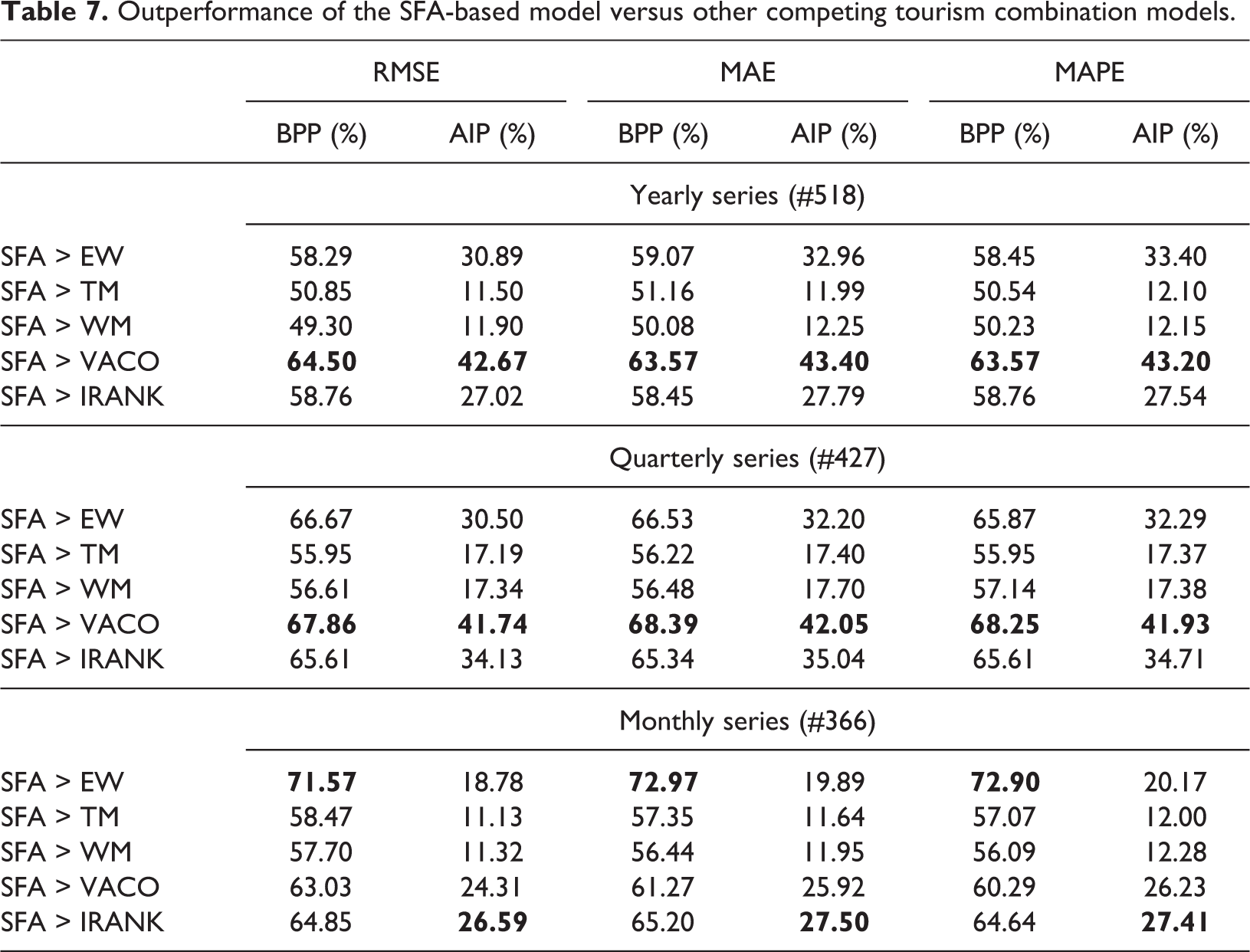
According to the result of the mean and the mean rank of the relative accuracy measures, following the ANOVA and Friedman’s tests, we confirm that the SFA-based tourism forecast combination model statistically significantly outperforms the competing models. We further investigate the extent of the outperformance. Table 7 shows the BPP and AIP of the three accuracy measures (RMSE, MAE and MAPE) for the SFA-based model with other competing models. BBI is the percentage of occasions that the SFA-based model performs better than certain competing forecast combination models, and AIP is the percentage of average improvement for all of the series for which the SFA-based model performs better than the competing forecast combination models. For example, considering the row ‘SFA > EW’ for the yearly series, the RMSE-related BBP is 58.29%, indicating that the number of occasions that the SFA-based model performs better than the EW model for the yearly series is 518 × 58.29% = 302 in terms of RMSE; the RMSE-related AIP is 30.89%, indicating an average improvement of 30.89% in the 302 yearly series. From Table 7, we see that the outperformance of the SFA-based forecast combination model is quite different for the time series with different frequencies and different accuracy measures. Taking the yearly series again as an example, the largest value of BPP is in the row ‘SFA > VACO’, whereas for the monthly series, it is in the row ‘SFA > EW’. Table 7 reveals that the majority of the BPP values are greater than 50% (the greatest value is 76.44%), which again illustrates that the SFA-based model is superior to the competing models. The performance enhancements of the SFA-based model, compared to EW and VACO, are much higher than those compared to the TM and WM models, findings that are supported by much of the related literature.

Table 7.

Outperformance of the SFA-based model versus other competing tourism combination models.

	RMSE		MAE		MAPE
	BPP (%)	AIP (%)	BPP (%)	AIP (%)	BPP (%)	AIP (%)
	Yearly series (#518)
SFA > EW	58.29	30.89	59.07	32.96	58.45	33.40
SFA > TM	50.85	11.50	51.16	11.99	50.54	12.10
SFA > WM	49.30	11.90	50.08	12.25	50.23	12.15
SFA > VACO	64.50	42.67	63.57	43.40	63.57	43.20
SFA > IRANK	58.76	27.02	58.45	27.79	58.76	27.54
	Quarterly series (#427)
SFA > EW	66.67	30.50	66.53	32.20	65.87	32.29
SFA > TM	55.95	17.19	56.22	17.40	55.95	17.37
SFA > WM	56.61	17.34	56.48	17.70	57.14	17.38
SFA > VACO	67.86	41.74	68.39	42.05	68.25	41.93
SFA > IRANK	65.61	34.13	65.34	35.04	65.61	34.71
	Monthly series (#366)
SFA > EW	71.57	18.78	72.97	19.89	72.90	20.17
SFA > TM	58.47	11.13	57.35	11.64	57.07	12.00
SFA > WM	57.70	11.32	56.44	11.95	56.09	12.28
SFA > VACO	63.03	24.31	61.27	25.92	60.29	26.23
SFA > IRANK	64.85	26.59	65.20	27.50	64.64	27.41

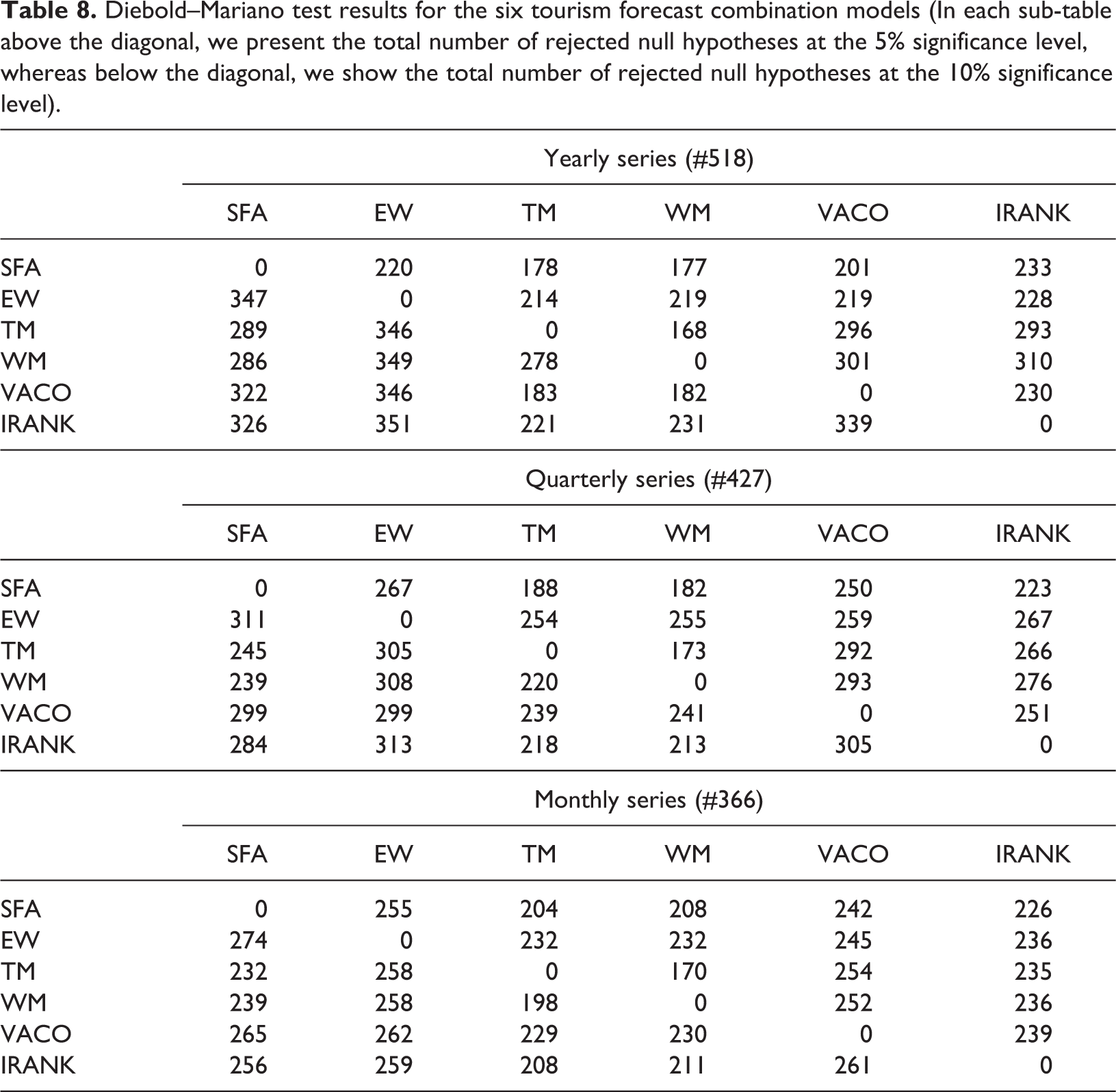
We also carry out the Diebold–Mariano test to compare the forecast accuracy between the SFA-based model and the five competing tourism forecast combination models. The null hypothesis of the Diebold–Mariano test is that there is an equal expected forecast performance for pairwise forecast combination models. The Diebold–Mariano test is executed to evert the time series, and the number of rejected null hypotheses for all of the time series with different frequencies are counted. Table 8 presents the results of the Diebold–Mariano test for the six forecast combination models. In each sub-table above the diagonal line of zeroes we present the total number of rejected null hypotheses at the 5% significance level. Below the diagonal, we show the total number of rejected null hypotheses at the 10% significance level. When the significance level is 5%, comparing the SFA-based model to the competing models, we conclude that the forecast performance of the SFA-based model is quite different for the majority of the monthly series values; for example, when compared with the EW model, 255 of 366 monthly series are statistically significant. However, the forecast performance of the SFA-based model is only different for a minority of the yearly and quarterly series. When the significance level is at 10%, the forecast performance of the SFA-based model is quite different from the other competing models for the majority of the time series with different frequencies; for example, when compared with the performance of the EW model, the SFA-based model performance is statistically significant for about 75% of the monthly series. From this table, we can conclude that the forecast performances of the five competing models are quite different.

Table 8.

Diebold–Mariano test results for the six tourism forecast combination models (In each sub-table above the diagonal, we present the total number of rejected null hypotheses at the 5% significance level, whereas below the diagonal, we show the total number of rejected null hypotheses at the 10% significance level).

	Yearly series (#518)
	SFA	EW	TM	WM	VACO	IRANK
SFA	0	220	178	177	201	233
EW	347	0	214	219	219	228
TM	289	346	0	168	296	293
WM	286	349	278	0	301	310
VACO	322	346	183	182	0	230
IRANK	326	351	221	231	339	0
	Quarterly series (#427)
	SFA	EW	TM	WM	VACO	IRANK
SFA	0	267	188	182	250	223
EW	311	0	254	255	259	267
TM	245	305	0	173	292	266
WM	239	308	220	0	293	276
VACO	299	299	239	241	0	251
IRANK	284	313	218	213	305	0
	Monthly series (#366)
	SFA	EW	TM	WM	VACO	IRANK
SFA	0	255	204	208	242	226
EW	274	0	232	232	245	236
TM	232	258	0	170	254	235
WM	239	258	198	0	252	236
VACO	265	262	229	230	0	239
IRANK	256	259	208	211	261	0

Lastly, we focus on the computational complexity of the SFA-based model and the five competing forecast combination models. Indeed, there is a trade-off between accuracy and computational complexity in the domain of forecasting. Although computers are faster and have better computer memory, computational complexity remains an important issue. There are two resources for the analysis of computational complexity: time complexity and space complexity. In this article, we use computational time (CT), defined as the total time needed to run a tourism forecast combination model, to measure the time complexity. To measure space complexity, we use memory usage (MU), defined as the size of the memory needed to run a model. Table 9 shows the results of the computational complexity for the six tourism forecast combination models. From this table, we see that the CT and MU for the six tourism forecast combination models are all in the same order of magnitude. One reasonable explanation is that the SFA-based model and the five competing forecast combination models are all linear combination models, not non-linear combination models. Furthermore, the CT and MU for the SFA-based model is higher than the SA-based models (EW, TM and WM) but lower than the OW-based models (VACO and IRANK). The SA-based model assigns constant weights for the individual tourism models, but the OW-based model must solve an optimization problem based on a function of forecast error-derived accuracy measures. The SFA-based model only needs to solve the Cobb–Douglas production function with determined inputs and outputs.

Table 9.

Results of analysis of computational complexity for the six tourism forecasting combination models.

	Yearly series (#518)		Quarterly series (#427)		Monthly series (#366)
	CT (s)	MU (Mb)	CT (s)	MU (Mb)	CT (s)	MU (Mb)
SFA	385.2	18.5	321.6	15.6	282.9	13.1
EW	314.9	16.7	259.6	15.1	222.5	14.7
TM	331.5	14.2	273.2	13.8	234.2	13.2
WM	334.7	16.4	275.9	15.7	236.5	14.5
VACO	423.6	30.6	349.2	23.2	299.3	21.6
IRANK	412.8	19.7	340.3	18.8	291.7	17.5

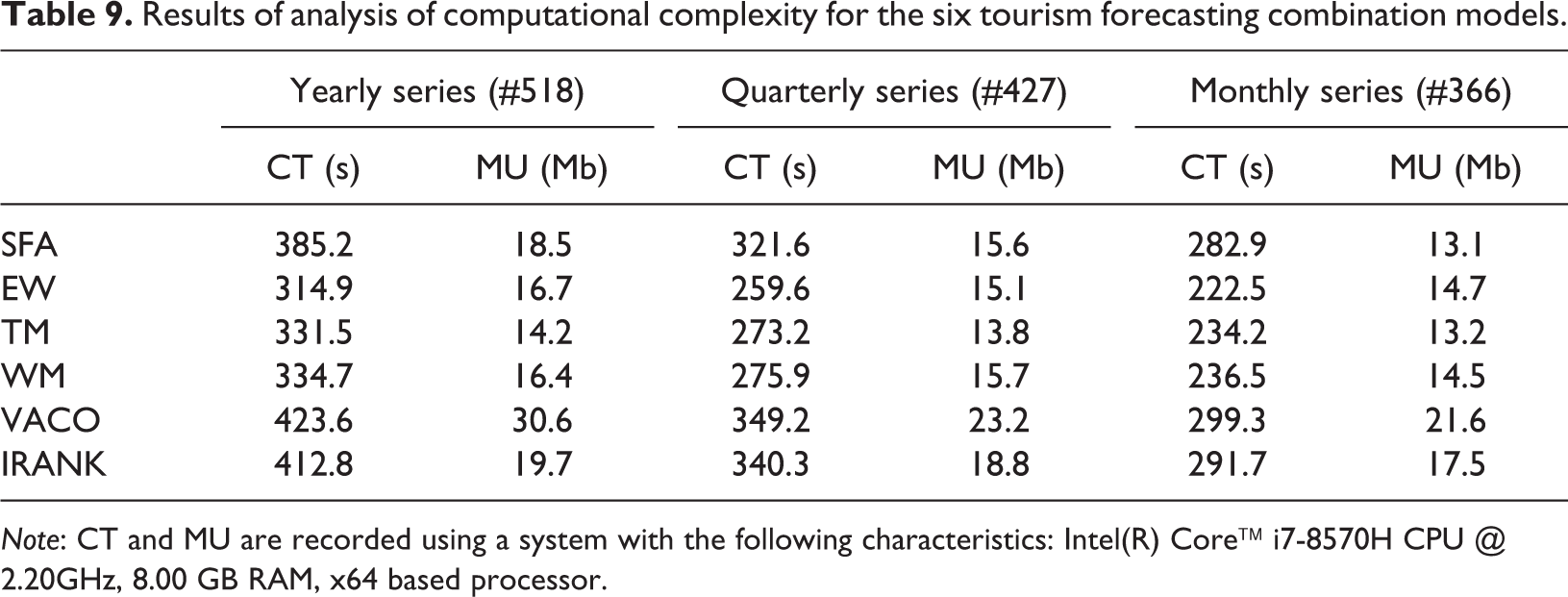
Note: CT and MU are recorded using a system with the following characteristics: Intel(R) Core™ i7-8570H CPU @ 2.20GHz, 8.00 GB RAM, x64 based processor.

Based on the experimental results of the multiple criteria performance indicators, we find that the SFA-based model statistically significantly outperforms the five competing forecast combination models for the majority of the time series in the tourism forecast competition data set. Furthermore, the results of the hypotheses’ three tests – the ANOVA, Friedman’s test and the Diebold–Mariano test – also statistically confirm and strengthen the finding.The computational complexity of the SFA-based model and the five competing forecast combination models are in the same order of magnitude, and it is indeed higher than that of the SA-based models (EW, TM and WM) but lower than that of OW-based models (VACO and IRANK). There are several reasons for this finding. First, because the SFA-based forecast combination model takes into account multiple accuracy measures, the performance evaluation for this model is more reliable and precise as multiple accuracy measures provide multifaceted information on the individual forecast model, and thus the combination weights generated by these performance evaluation results are much more rational and comprehensive. Second, multiple accuracy measures can complement each other as different accuracy measures have their different advantages and disadvantages, leading to more robust weights for the individual forecast model. Third, unlike traditional combination methods that usually combine two individual forecast models, in this experiment we use 13 individual models to form the forecast combination. Different individual models might capture particular patterns of the target time series, so a combination of these forecast models comes closer to representing the true patterns of the target time series. Fourth, the SFA-based model is a linear forecast combination model, so it has the same order of magnitude for computational complexity. In conclusion, the forecast performance of the SFA-based model is substantially better than that of the other competing models.

Conclusion and discussion

In this article, we propose a novel performance-based forecast combination model for tourism forecasting that takes multiple accuracy measures into account. In particular, we consider forecasting performance evaluation under multiple accuracy measures as an MCDM problem and use the classical SFA technique to solve the problem. To demonstrate the effectiveness of the proposed tourism forecast combination model, we conduct a comprehensive study to investigate its forecasting performance by using the tourism forecast competition data set. We empirically show that the performance-based forecast combination model statistically significantly outperforms the five competing forecast combination models in most cases. The proposed model provides us with a good solution to identify suitable weights for individual models as it takes into account multiple accuracy measures, and the SFA technique guarantees the rationality and preciseness of the performance evaluation results for the individual tourism forecast models. At the same time, the performance-based model does not increase the computational complexity required as it is a linear combination paradigm. This research enhances the tourism forecast combination literature as the traditional linear combination model only considers SA weight and the so-called OW, which usually depends solely on one forecast error derived from an accuracy measure (Chan and Pauwels, 2018). The research also presents a comprehensive comparison of the forecast combination techniques, as we build 13 individual tourism forecast models and five forecast combination models from 1311 tourism time-series data.

Although we have conducted a comprehensive study to demonstrate the effectiveness of the performance-based forecast combination model, some shortcomings in our research should be considered in future studies. First, the selection of the accuracy measures and individual forecast models used in the MCDM framework is a big challenge. There is no standard well-accepted criterion for the selection of accuracy measures in the traditional literature, primarily because a bewildering number of accuracy measures have been proposed to evaluate forecast models. Most of these accuracy measures are not generally applicable and can produce misleading results as different accuracy measures evaluate different aspects of forecast errors. Thus, the choice of the most suitable accuracy measure remains controversial (Davydenko and Fildes, 2013). The major work of our research is to empirically investigate whether the proposed performance-based combination model is feasible, so we have chosen just four accuracy measures to illustrate our proposed model’s effectiveness. However, the selection of appropriate accuracy measures in the MCDM framework is an interesting topic and a possible path for future work. Similarly, we use 13 individual tourism forecast models to form the forecast combination, and indeed the 13 models guarantee the diversification of individual models to some extent as they come from four categories: exponential smoothing, ARIMA, complex methods and simple methods. However, the models all belong to traditional statistical methods, and artificial intelligence techniques, such as ANN and SVM, have not been included in our study. Experiments should be conducted to tackle such artificial intelligence techniques in future research. These problems could be the start of further studies within the realm of tourism forecasting.

Footnotes

Declaration of conflicting interests

The author(s) declared no potential conflicts of interest with respect to the research, authorship, and/or publication of this article.

Funding

The author(s) disclosed receipt of the following financial support for the research, authorship, and/or publication of this article: This research study is supported by the National Natural Science Foundation of China (no. 71701172 and 71601190).

ORCID iD

Xian Cheng

Note

References

Adhikari

(2015) A neural network based linear ensemble framework for time series forecasting. Neurocomputing 157: 231–242.

Aigner

Lovell

Schmidt

(1977) Formulation and estimation of stochastic frontier production function models. Journal of Econometrics 6(1): 21–37.

Aiolfi

Timmermann

(2006) Persistence in forecasting performance and conditional combination strategies. Journal of Econometrics 135(1–2): 31–53.

Anaya

Pollitt

(2017) Using stochastic frontier analysis to measure the impact of weather on the efficiency of electricity distribution businesses in developing economies. European Journal of Operational Research 263(3): 1078–1094.

Andrawis

Atiya

El-Shishiny

(2011) Combination of long term and short term forecasts, with application to tourism demand forecasting. International Journal of Forecasting 27(3): 870–886.

Armstrong

(2001) Principles of Forecasting: A Handbook for Researchers and Practitioners, vol. 30. Springer Science & Business Media.

Armstrong

Collopy

(1992) Error measures for generalizing about forecasting methods: empirical comparisons. International Journal of Forecasting 8(1): 69–80.

Assimakopoulos

Nikolopoulos

(2000) The theta model: a decomposition approach to forecasting. International Journal of Forecasting 16(4): 521–530.

Athanasopoulos

Hyndman

Song

, et al. (2011) The tourism forecasting competition. International Journal of Forecasting 27(3): 822–844.

10.

Azevedo

Campos

LMS

(2016) Combination of forecasts for the price of crude oil on the spot market. International Journal of Production Research 54(17): 5219–5235.

11.

Bates

Granger

CWJ

(1969) The combination of forecasts. OR 20(4): 451–468.

12.

Cai

Wang

, et al. (2016) A spatiotemporal correlative k-nearest neighbor model for short-term traffic multistep forecasting. Transportation Research Part C: Emerging Technologies 62: 21–34.

13.

Cang

(2011) A non-linear tourism demand forecast combination model. Tourism Economics 17(1): 5–20.

14.

Cang

(2014) A combination selection algorithm on forecasting. European Journal of Operational Research 234(1): 127–139.

15.

Chan

Witt

Lee

YCE

, et al. (2010) Tourism forecast combination using the CUSUM technique. Tourism Management 31(6): 891–897.

16.

Chan

Pauwels

(2018) Some theoretical results on forecast combinations. International Journal of Forecasting 34(1): 64–74.

17.

Chan

Stock

Watson

(1999) A dynamic factor model framework for forecast combination. Spanish Economic Review 1(2): 91–121.

18.

Charoenrat

Harvie

(2014) The efficiency of SMEs in Thai manufacturing: a stochastic frontier analysis. Economic Modelling 43: 372–393.

19.

Chen

(2011) Combining linear and nonlinear model in forecasting tourism demand. Expert Systems with Applications 38(8): 10368–10376.

20.

Chen

Lee

(2015) A weighted LS-SVM based learning system for time series forecasting. Information Sciences 299: 99–116.

21.

Coleman

Swanson

(2007) On MAPE-R as a measure of cross-sectional estimation and forecast accuracy. Journal of Economic and Social Measurement 32(4): 219–233.

22.

Coshall

Charlesworth

(2011) A management orientated approach to combination forecasting of tourism demand. Tourism Management 32(4): 759–769.

23.

Crone

Hibon

Nikolopoulos

(2011) Advances in forecasting with neural networks? Empirical evidence from the NN3 competition on time series prediction. International Journal of Forecasting 27(3): 635–660.

24.

Davydenko

Fildes

(2013) Measuring forecasting accuracy: the case of judgmental adjustments to SKU-level demand forecasts. International Journal of Forecasting 29(3): 510–522.

25.

De Livera

Hyndman

Snyder

(2011) Forecasting time series with complex seasonal patterns using exponential smoothing. Journal of the American Statistical Association 106(496): 1513–1527.

26.

dos Santos

RDV

Vellasco

(2015) Neural expert weighting: a new framework for dynamic forecast combination. Expert Systems with Applications 42(22): 8625–8636.

27.

Hailu

Tanaka

(2015) A ‘true’ random effects stochastic frontier analysis for technical efficiency and heterogeneity: evidence from manufacturing firms in Ethiopia. Economic Modelling 50: 179–192.

28.

Hassani

Silva

Antonakakis

, et al. (2017) Forecasting accuracy evaluation of tourist arrivals. Annals of Tourism Research 63: 112–127.

29.

Hirashima

Jones

Bonham

, et al. (2017) Forecasting in a mixed up world: nowcasting Hawaii tourism. Annals of Tourism Research 63: 191–202.

30.

Hyndman

King

Pitrun

, et al. (2005) Local linear forecasts using cubic smoothing splines. Australian & New Zealand Journal of Statistics 47(1): 87–99.

31.

Hyndman

Koehler

(2006) Another look at measures of forecast accuracy. International Journal of Forecasting 22(4): 679–688.

32.

Jiao

Chen

(2018) Tourism forecasting: a review of methodological developments over the last decade. Tourism Economics 25(3): 469–492.

33.

Jose

VRR

Winkler

(2008) Simple robust averages of forecasts: some empirical results. International Journal of Forecasting 24(1): 163–169.

34.

Kumbhakar

Lovell

(2003) Stochastic frontier analysis. Cambridge: Cambridge university press.

35.

Chen

Wang

, et al. (2018) Effective tourist volume forecasting supported by PCA and improved BPNN using Baidu index. Tourism Management 68: 116–126.

36.

Liu

Wang

, et al. (2018) Hot topics and emerging trends in tourism forecasting research: a scientometric review. Tourism Economics 25: 448–468.

37.

Makridakis

Andersen

Carbone

, et al. (1982) The accuracy of extrapolation (time series) methods: results of a forecasting competition. Journal of Forecasting 1(2): 111–153.

38.

Makridakis

Hibon

(2000) The M3-Competition: results, conclusions and implications. International Journal of Forecasting 16(4): 451–476.

39.

Meeusen

van Den Broeck

(1977) Efficiency estimation from Cobb-Douglas production functions with composed error. International Economic Review 18: 435–444.

40.

Petropoulos

Hyndman

Bergmeir

(2018) Exploring the sources of uncertainty: why does bagging for time series forecasting work? European Journal of Operational Research 268(2): 545–554.

41.

Podsiadlo

Rybinski

(2016) Financial time series forecasting using rough sets with time-weighted rule voting. Expert Systems with Applications 66: 219–233.

42.

Prestwich

Rossi

Armagan Tarim

, et al. (2014) Mean-based error measures for intermittent demand forecasting. International Journal of Production Research 52(22): 6782–6791.

43.

Sermpinis

Dunis

Laws

, et al. (2012) Forecasting and trading the EUR/USD exchange rate with stochastic neural network combination and time-varying leverage. Decision Support Systems 54(1): 316–329.

44.

Shen

Song

(2008) An assessment of combining tourism demand forecasts over different time horizons. Journal of Travel Research 47(2): 197–207.

45.

Shen

Song

(2011) Combination forecasts of international tourism demand. Annals of Tourism Research 38(1): 72–89.

46.

Shenstone

Hyndman

(2005) Stochastic models underlying Croston’s method for intermittent demand forecasting. Journal of Forecasting 24(6): 389–402.

47.

Song

Witt

Wong

, et al. (2009) An empirical study of forecast combination in tourism. Journal of Hospitality & Tourism Research 33(1): 3–29.

48.

Stewart

(1996) Relationships between data envelopment analysis and multicriteria decision analysis. Journal of the Operational Research Society 47: 654–665.

49.

Sun

Wei

Tsui

, et al. (2019) Forecasting tourist arrivals with machine learning and internet search index. Tourism Management 70: 1–10.

50.

Svetunkov

Boylan

(2019) State-space ARIMA for supply-chain forecasting. International Journal of Production Research. DOI: 10.1080/00207543.2019.1600764.

51.

Swanson

Tayman

Barr

(2000) A note on the measurement of accuracy for subnational demographic estimates. Demography 37(2): 193–201.

52.

Timmermann

(2006) Chapter 4 forecast combinations. In: Elliott

CWJGG

Timmermann

(eds) Handbook of Economic Forecasting. Amsterdam: Elsevier, vol 1, pp. 135–196.

53.

Turner

Witt

(2001) Forecasting tourism using univariate and multivariate structural time series models. Tourism Economics 7(2): 135–147.

54.

Van Gils

Ramaekers

Caris

, et al. (2017) The use of time series forecasting in zone order picking systems to predict order pickers’ workload. International Journal of Production Research 55(21): 6380–6393.

55.

Wan

Song

(2018) Forecasting turning points in tourism growth. Annals Of Tourism Research 72: 156–167.

56.

Wong

KKF

Song

Witt

, et al. (2007) Tourism forecasting: To combine or not to combine? Tourism Management 28(4): 1068–1078.

57.

Song

Shen

(2017) New developments in tourism and hotel demand modeling and forecasting. International Journal of Contemporary Hospitality Management 29(1): 507–529.

58.

Zionts

(1992) Some thoughts on research in multiple criteria decision making. Computers & Operations Research 19(7): 567–570.