Does tourism promote economic growth? A fractionally integrated heterogeneous panel data analysis

Abstract

In this article, we analyse whether tourism promotes economic growth using a general dynamic panel data model that incorporates individual and interactive fixed effects and allows for contemporaneous correlation in model innovations. The empirical study is based on quarterly series of GDP and tourist arrivals for 14 European countries covering the period from 1995 to 2019. Results indicate that the case for a positive long-run relationship between tourism and economic growth is rather weak, being slightly stronger for the period prior to the global economic and financial crisis from 2007 to 2010. When applying panel fractional cointegration techniques, we find evidence in favour of the tourism-led growth hypothesis (TLGH) for the full sample mainly for North European countries. For the pre-crisis period, on the other hand, we find evidence in favour of the TLGH for the relevant tourist destinations Spain and France.

Keywords

fractional integration and cointegration panel data recent financial crisis tourism-led growth hypothesis

Introduction

In general, tourism exerts a positive impact on economic growth. Tourism creates employment opportunities, enlarges the consumer markets, promotes export trade and generates foreign exchange earnings (Saleh et al., 2015). In 2019, the number of international tourists grew by 3.8% to 1462 million, while in Europe, tourist arrivals grew by 4%. However, the coronavirus (COVID-19) crisis has completely changed this scenario of continuous growth of international tourism, and large declines are expected for 2020 and 2021. Considering that many European countries such as France, Italy and Spain receive large foreign income from international tourism, the pandemic is expected to have a large impact on their GDP. So, a rigorous and in-depth analysis of the impact of the tourism sector on European GDP is needed for a proper quantification of the magnitude of the crisis. This would help policymakers and stakeholders in the tourism sector to design a recovery plan and to avoid a larger impact from a potential worsening of the pandemic. Indeed, since the tourism sector is highly dependent on international mobility and economic crises, it becomes crucial to understand whether the effects of shocks on tourism are permanent or transitory and to properly model the nexus between tourism and economic growth. The present article aims at contributing to the extensive literature on the tourism led-growth hypothesis (TLGH) by exploring the link between tourism and economic growth in a panel data set of countries using fractional cointegration techniques. This technique has not been previously applied to explore the TLGH and can improve on both fractional methods in a time-series context and standard cointegration methods in a panel context.

First, it is noteworthy that standard cointegration methods might be too restrictive. In particular, in the time-series literature, both unit root tests and cointegration analysis are known to perform poorly in the presence of fractional integration (see, e.g. Dittman, 2000, Gil-Alana et al., 2014). In consequence, conclusions drawn from these methods might not be appropriate. This issue is important, insofar as the existence of a long-run relationship could then be associated with a slow reversion to equilibrium due to the persistence of shocks. In the context of a large decline in the tourism sector, such as the one caused by the global financial and economic crisis or the COVID-19 crisis, it is not only relevant to check the validity of techniques that quantify the impact of inbound tourism on countries’ GDP but also the type and duration of the adjustment after a shock. Fractional methods, on the other hand, are more general and flexible, have greater power against unit roots than the standard techniques have and accommodate a slow rate of mean reversion. The advantage of the fractional integration analysis is then that it allows exploring the degree of the persistence of shocks to the system. Thus, it might lead to more accurate results. The only antecedent in the application of fractional cointegration techniques to the TLGH is the article by Pérez-Rodríguez et al. (2020). It applies fractional integration and cointegration analyses to explore the validity of the TLGH but in a time-series context.

Second, panel data methods – in contrast to time-series methods – allow for fixed effects, that is, idiosyncratic differences between the individual units (here, countries). Several dynamic panel methods on large panels have been proposed, including pooled mean group estimation proposed by Pesaran et al. (1999), fully modified ordinary least squares (OLS) estimation by Pedroni (1999, 2001, 2004) or the panel dynamic OLS estimation by Pedroni (2001) and Mark and Sul (2003), to allow for interactions between cross sections. These methods have been applied, among others, to analyse the link between international tourism and trade (Santana-Gallego et al., 2011). However, this literature typically ignores cross section dependence of errors. More recently, Pesaran (2006) proposed the common correlated effects (CCEs), and Chudik and Pesaran (2015) extended common correlated effects estimation (DCCE) to the context of heterogeneous dynamic panel data models which allow for cross section dependence of errors. Some recent papers have used these approaches on tourism such as Harb and Bassil (2020) using CCE in a gravity analysis of tourism flows and Meo et al. (2020) using DCCE to analyse water resources and tourism development in South Asia. Drisatkis (2012) and Mello-Sampayo and Sousa-Vale (2012) applied panel cointegration methods to the analysis of the TLGH. However, as aforementioned, the persistence in system shocks is rather inflexible with standard cointegration methods.

The recent literature on panel fractional cointegration relaxes this assumption. It, thus, combines the advantages of both – allowance for heterogeneity and fixed effects via the panel structure and more flexible persistence via fractional cointegration. In particular, the fractionally integrated heterogeneous panel data approach proposed by Ergemen (2019) accommodates general stationary or nonstationary long-range dependence through interactive fixed effects and innovations, removing the necessity to perform a priori unit root or stationarity testing.

This article is the first to apply these fractional integration and cointegration techniques for panel data to study the validity of the TLGH. Although we do not have enough data yet to quantify the impact of the COVID-19 crisis on the tourism sector, the present research explores how the tourism sector contributes to economic growth for a selected group of European countries and analyses the impact of another crisis – the recent global financial and economic crisis – on the tourism sector. To justify the adoption of strategic policies to promote tourism as a driver of economic growth, policymakers should not only take into account the speed of adjustment towards equilibrium but also consider whether the causal link between tourism and growth is affected by the type of adjustment. Consequently, allowing more general persistence in the form of long memory will help tourism operators and policymakers to develop effective planning strategies.

In particular, in the empirical analysis, we use quarterly data on inbound tourism (arrivals) and GDP for a sample of 14 European countries for the period 1995–2019. The choice of tourist arrivals rather than tourism expenditure is dictated by data availability. Yet, the latter might be the better proxy for tourism activity since it takes into account idiosyncratic features such as the duration of the stay or the type of tourism. In particular, higher expenditures may be the result of a longer stay due to a longer distance between the origin and destination country or the type of destinations. For instance, tourists usually spend more money in urban or cultural destinations while the duration of the holidays is larger in beach resorts or the countryside, where tourists spend less money. However, for the present analysis, large and homogeneous data for inbound tourism in a selected group of European countries are only available for tourist arrivals.

The rest of this article is organized as follows. The second section reviews the literature. The third section gives a short overview of standard integrated panel methods and describes the fractional panel data methodology. The fourth section presents the empirical analysis and the main results. Finally, the fifth section summarizes the main conclusions.

Literature review

The TLGH and standard econometric methods

There is a large literature on the effect of tourism on economic growth, in particular, studying the validity of the so-called tourism-led growth hypothesis (TLGH). Much of the empirical evidence supports the TLGH, although results are sensitive to a number of factors related to country data, specification, estimation characteristics and time span (Comerio and Strozzi, 2019; Nunkoo et al., 2019; Pablo-Romero and Molina, 2013).

Several econometric techniques have been used to explore the TLGH, from cross-sectional and time-series models to panel data models, with a more global focus. Among the econometric methods, most are time-series models and fewer are cross-sectional and panel data studies. Brida et al. (2016) reviewed 95 selected papers that explored the link between tourism and economic growth among which only 12 apply panel data techniques. Indeed, the number of investigated countries is limited and unbalanced and the analysis has been mainly applied to destinations with a high weight of the tourism sector which exerts a positive impact on economic growth. Similarly, Castro-Nuño et al. (2013) review 13 empirical studies of the TLGH using panel data and also agree that there are insufficient studies applying panel data techniques. In general, the empirical literature on the TLGH is extensive in both type of analysed countries and used econometric methodology. Regarding the econometric methods, the literature has employed cross-sectional models, time-series models and panel data models (Castro-Nuño et al., 2013).

First, most of the literature on the TLGH applies time-series analysis. Many researchers have focused on the existence of a long-run relationship between tourism and economic growth and on studying the corresponding causality between GDP and tourism. Both long-run and causality analyses are of strategic importance for policymakers. For example, a complementary long-run relationship, with unidirectional causality from tourism to growth, would justify the adoption of policies to promote tourism as a driver of economic growth (regional and/or national). In this framework, studies using standard cointegration techniques and Granger causality tests for Mediterranean countries are Balaguer and Cantavella-Jordá (2002) and Dritsakis (2004), among others; and Asia and Pacific countries are Narayan and Prasad (2003), Durbarry (2004), Narayan (2004) and Oh (2005), among others. Most of the country studies employed Granger causality tests and provided evidence that both tourism-led growth and growth-led tourism development occurs. However, it is noteworthy that other time-series methods have also been used to analyse the relationship between tourism and growth, such as time-varying models (Antonakakis et al., 2015; Balcilar et al., 2014), nonlinear models (Brida et al., 2015; Phiri, 2016; Wang, 2012), copula-based generalized autoregressive conditional heteroskedasticity (GARCH) models (Pérez-Rodríguez et al., 2015) or quantile methods (Shahzad et al., 2017). As aforementioned, the only article that performs a fractional cointegration analysis is Pérez-Rodríguez et al. (2020), but in a time-series context for a group of European countries. In their empirical exercise, they found evidence of cointegration only in very restricted cases such as for Italy for the overall period and for Italy and Spain for the pre-crisis period (1990–2007). Therefore, the validity of the TLGH is less clear-cut with this methodology than with traditional cointegration analysis.

Second, only few articles apply cross-sectional techniques (see, for instance Brau et al., 2007; Figini and Vici, 2010). In general, these studies find evidence in favour of a positive relation between export growth and economic growth, but they fail to detect causality from one variable to the other one due to the nature of data, that is, the absence of a time dimension.

Third, there is a growing literature applying panel data techniques since they allow exploring the validity of the TLGH for a large group of countries and/or regions, and consequently, more general conclusions can be drawn. So far, standard panel data methods (static and dynamic) and panel cointegration analysis and causality analysis have been used. As example of the former, Eugenio-Martin et al. (2004) estimated the relationship between economic growth and tourism for Latin American countries for 1985–1998 by panel data techniques. They observe that tourism growth is associated with economic growth only in low- and medium-income countries but not in high-income countries. Sequeira and Nunes (2008) are the first to evaluate the worldwide impact of tourism, using panel data techniques dealing with endogeneity and following the empirical economic growth literature (see also Cortés-Jiménez, 2008; Fayissa et al., 2008; Holzner, 2011; Narayan et al., 2010; Seetenah, 2011). As example of the latter, Tang and Tan (2018) test the TLGH at a global level and obtain that tourism contributes to economic growth, but the effect varies across countries at different levels of income and institutional qualities. Indeed, the impact of tourism on economic growth is larger for high-income countries. The authors found solid empirical evidence of panel cointegration relationships between tourism development and GDP. Lee and Chang (2008) used a heterogeneous panel cointegration technique to reinvestigate the long-run co-movements and causal relationships between tourism development and economic growth for Organisation for Economic Co-operation and Development (OECD) and non-OECD countries (including those in Asia, Latin America and sub-Sahara Africa) for the 1990–2002 period. Tourism development has a greater impact on GDP in non-OECD countries than in OECD countries. Drisatkis (2012) applies panel cointegration analysis to explore the TLGH for seven Mediterranean countries, including France, Spain, Italy and Greece, as we do in our analysis and finds evidence in favour of the TLGH. Salifou and Haq (2017) also apply standard panel cointegration techniques to test the validity of the TLGH for 11 countries of the Economic Community of West African States. Paramati et al. (2017) apply robust panel econometric techniques to examine the dynamic relationships among tourism, economic growth and carbon monoxide² emissions. All these authors obtain a positive link between tourism and economic growth. Importantly, all these articles apply standard cointegration techniques to explore the long-run relationship between tourism and economic growth. Thus, as previously mentioned, fractional cointegration techniques in a panel data context have not been used to analyse the TLGH. Consequently, the main contribution of this article is to provide such analysis of the long-range dependence in the joint dynamic behaviour of GDP and tourism and, by doing so, to provide a more accurate picture.

Both Paramati et al (2017) and Tang and Tan (2018) highlight the relevance of classifying countries into developed and developing for a proper analysis of this issue. Indeed, Tang and Tan (2018) obtained that the growth effect of tourism depends on the level of income of the tourist-destination country and its institutional quality. More specifically, high-income countries’ growth is impacted by tourism to a larger positive degree than lower income countries’ growth is. This is due to the greater presence of tourism-related eco-system in high-income countries that could effectively attract inbound tourists. For that reason, in our research, we focus on a set of developed countries, specifically a selected group of European countries with different levels of tourism development.

For the specific case of the TLGH in European countries, Mello-Sampayo and Sousa-Vale (2012) apply likelihood-based panel cointegration techniques to examine the existence of a long-run relationship between GDP and tourism for a panel for the period 1988–2010. Interestingly, these authors obtained that tourism shows a long-run relationship with economic growth, but its impact on the long-run economic growth is much smaller than suggested by its share on GDP. In particular, tourism development has a higher impact on GDP in North than in South European countries. Antonakakis et al. (2015) obtain, for a group of six European countries, that the tourism–economy relationship is not stable over time for all countries in terms of both its magnitude and direction. Moreover, they show that the above-mentioned relationship tends to exhibit a change in its magnitude and/or direction during major economic events. Indeed, they estimate a structural break in the tourism–economic growth link during and after the Great Recession. Consequently, it becomes crucial to properly understand the nature of the relationship between tourism and economic growth and the persistence of the effect after a shock, such as the COVID-19 crisis.

To conclude, most of the articles applying time-series techniques find evidence in favour of the TLGH (Brida et al., 2016). However, the empirical estimates of the magnitude of the effect of tourism on economic growth are mixed. This diversity might be a consequence of assuming integer orders in the standard integration and cointegration methods, while the equilibrium errors might in fact be fractionally integrated, with GDP and tourism being fractionally cointegrated (Pérez-Rodríguez et al., 2020). Therefore, the empirical validity of the TLGH still deserve further research and a more detailed exploration of this topic is essential to design policy recommendations, especially during crisis episodes.

Fractional cointegration and TLGH

Long memory, or long-range dependence, describes the correlation structure of data series presenting long lags. In other words, long memory represents persistent temporal dependence between observations, even if they are far apart. In this case, data series are characterised by cyclical but not periodic patterns. There exists an important body of literature on fractional cointegration methods (Gil-Alana and Hualde, 2009). Fractional cointegration describes a long-run relationship between two trending variables with the equilibrium error being persistent, but less so than the variables themselves.

To the best of our knowledge, only few articles have applied fractional cointegration techniques to tourism-related data series. For example, Fischer and Gil-Alana (2009) studied fractional cointegration between trade and tourism to analyse the association between German tourism in Spain and German imports of Spanish wine. Since their data series have different orders of integration and, thus, different stochastic properties, these authors proposed a method based on long memory regression models, in which tourism was assumed to be an exogenous factor. More recently, Pérez-Rodríguez et al. (2020) have explored the validity of the TLGH applying fractional cointegration techniques. To do so, they studied the long-run relationship between GDP and tourist arrivals, using a two-step strategy. First, they applied fractional cointegration methods and, then, they tested the null hypothesis of no cointegration against fractionally cointegrated alternatives. Moreover, they compared their results with those obtained using standard cointegration methods. For the empirical analysis, they used seasonally adjusted quarterly data for GDP and tourist arrivals for seven European countries from 1990 to 2018. Evidence of fractional cointegration was found only in very restricted cases. Therefore, the validity of the TLGH is less clear-cut when this methodology is applied.

Fractional panel data models have so far not been applied to tourism series. In fact, even at a methodological level, only few articles study fractional long-range dependence in the panel data context. Hassler et al. (2011) proposed a test for memory in fractionally integrated panels. Robinson and Velasco (2015) employed different estimation techniques to obtain efficient inference on the memory parameter in a fractional panel setting with fixed effects. Extending the latter, Ergemen and Velasco (2017) incorporated cross-section dependence and exogenous covariates to estimate slope and memory parameters in a single-equation setting, which enables disclosing possible cointegrating relationships between the unobserved independent idiosyncratic components. More recently, Ergemen (2019) has proposed a general dynamic panel data model that incorporates individual and interactive fixed effects allowing for contemporaneous correlation in model innovations. The model accommodates general stationary or nonstationary long-range dependence through interactive fixed effects and innovations, removing the necessity to perform a priori unit root or stationarity testing. Moreover, persistence in innovations and interactive fixed effects allows for cointegration; this model, further, features innovations with vector-autoregressive dynamics and accommodates deterministic trends.

In this article, we contribute to the empirical literature on the TLGH using panel data methods in a fractional cointegration framework.

Standard panel cointegration and fractionally integrated heterogeneous panel data model

Standard panel cointegration model

In this section, we provide a short summary of the (standard) panel cointegration test proposed by Pedroni (1999, 2004) and the corresponding estimator of the panel cointegration relationship (Pedroni, 2001). The test is an extension of the Engle and Granger (1987) cointegration test to a panel setup. In particular, allowing for heterogeneous intercepts and trend coefficients across cross-sections, consider:

y_{i t} = α_{i} + \partial_{i} t + {β^{'}}_{i 0} x_{i t} + e_{i t}, i = 1, ..., N, t = 1, ..., T

where $y_{i t}$ is the dependent variable of order I(1) and $x_{i t}$ is a m × 1 vector of I(1) explanatory variables. $α_{i}$ is an individual-specific fixed effects and $\partial_{i}$ denotes an individual-specific trend effect. Under the null of no-cointegration, $e_{i t}$ is of order I(1), while under the alternative of cointegration, it is of order I(0). The test consists in testing whether the residuals of equation (1) are I(1) by the following auxiliary regression:

e_{i t} = ρ_{i} e_{i t - 1} + \sum_{j = 1}^{p} ψ_{i j} Δ e_{i t - j} + v_{i t}, i = 1, ..., N

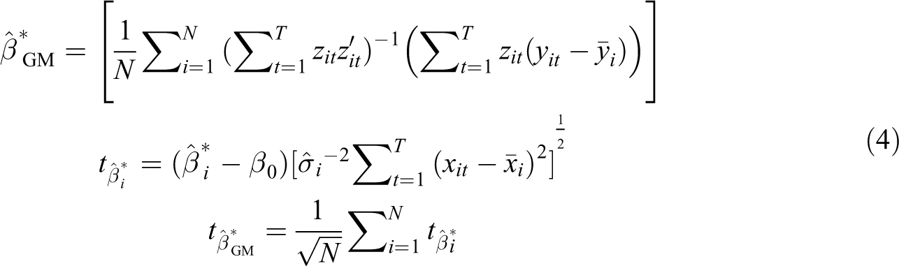
for each cross-section. The null hypothesis is $ρ_{i} = 1$ , while the homogenous alternative is $ρ_{i} = ρ < 1$ and the heterogeneous alternative is $ρ_{i} < 1$ for all i. Pedroni (2001) proposes several statistics constructed from the residuals in equation (1), all distributed as N(0,1).¹

After establishing panel cointegration, the slope coefficient in the cointegration relationship needs to be estimated. Here, we consider Pedroni’s (2001) panel dynamic ordinary least squares (DOLS) estimator. To estimate the dynamic model in equation (1), Pedroni proposed the following single-equation estimate of the cointegration vector: regress in each individual panel:

y_{i t} = α_{i} + \partial_{i} t + β_{i} x_{i t} + \sum_{j = - p}^{p} γ_{i j} Δ x_{i t - j} + μ_{i t}^{*}, i = 1, ..., N, t = 1, ..., T

where p is the number of lags and leads in the DOLS regression. This provides us with estimates of the individual slope parameters. The next step is to average the slope coefficients and associated t statistics over the entire panel, leading to the following group mean estimator:

\begin{matrix} {\hat{β}}^{*}_{GM} = [\frac{1}{N} \sum_{i = 1}^{N} {(\sum_{t = 1}^{T} z_{i t} z'_{i t})}^{- 1} (\sum_{t = 1}^{T} z_{i t} (y_{i t} - {\bar{y}}_{i}))] \\ t_{{\hat{β}}^{*}_{i}} = ({\hat{β}}^{*}_{i} - β_{0}) {[{\hat{σ}}_{i}^{- 2} \sum_{t = 1}^{T} {(x_{i t} - {\bar{x}}_{i})}^{2}]}^{\frac{1}{2}} \\ t_{{\hat{β}}^{*}_{GM}} = \frac{1}{\sqrt{N}} \sum_{i = 1}^{N} t_{{\hat{β}}^{*}_{i}} \end{matrix}

where $z_{i t}$ denotes the vector of regressors (including leads and lags of $Δ x_{i t}$ ) and ${\hat{σ}}_{i}^{2}$ is a long-run variance estimate of $μ_{i t}^{*}$ such as Newey and West (1987)’s heteroscedasticity and autocorrelation consistent method based on the Bartlett Kernel.

A fractionally integrated heterogeneous panel data model

In this section, we present the fractionally integrated heterogeneous panel data model proposed by Ergemen (2019). This model features fixed effects, persistent common factors allowing for cross-section dependence and potentially correlated persistent innovations. In this model, both regression errors and common factors are fractionally integrated and covariates are allowed to be endogenous through those unobserved common factors and through their innovations. Persistence arises from fractional integration, being, thus, an alternative to dynamic autoregressive panel data models. This fractional class of modelling nests the standard I(0) and I(1) cases and eliminates the necessity of preliminary unit root or stationarity testing, such as it is required in autoregressive modelling. Moreover, parameter estimates and related test statistics have standard distributions, unlike in the I(1) case. This model extends the factor structure used by Pesaran (2006) and the corresponding CCE estimation and extends previous work by Ergemen and Velasco (2017) insofar as it allows for contemporaneous correlation of the innovations and can feature factors with different memory parameters.

The general panel cointegrating regression model of Ergemen (2019) can be written as:

\begin{array}{l} y_{i t} = α_{i} + {β^{'}}_{i 0} x_{i t} + λ_{i}^{'} f_{t} + Δ_{t}^{- d_{i 0}} e_{1 i t}, i = 1, ..., N, t = 1, ..., T \\ x_{i t} = μ_{i} + γ'_{i} f_{t} + Δ_{t}^{- ϑ_{i 0}} e_{2 i t} \end{array}

where $y_{i t}$ is the endogenous variable, $x_{i t}$ is a vector of potentially endogenous covariates, $f_{t}$ is an m × 1 vector of unobserved common factors which is fractionally integrated of order $ω_{i}$ ( $f_{t} \sim I (ω_{i})$ ), i = 1,…, m; $λ_{i}, γ_{i}$ are vectors of factor loadings, determining the degree to which cross section units depend on the common factors; $e_{1 i t}$ and $e_{2 i t}$ are potentially correlated covariance stationary idiosyncratic shocks. Their short-memory dynamics are captured by a VAR(1) process. $d_{i 0}$ denotes the residual integration order. $ϑ_{i 0}$ denotes the memory of the defactored (unobserved) explanatory variable. The observed series’ memory is $max {ϑ_{i 0}, {max}_{i} ω_{i}}$ for $x_{i t}$ and $max {ϑ_{i 0}, d_{i 0}, {max}_{i} ω_{i}}$ for $y_{i t}$ . $α_{i}$ and $μ_{i}$ are covariate-specific fixed effects, and L is the lag operator. $Δ^{δ} = \sum_{j = 0}^{\infty} π_{j} (δ) L^{j}, π_{j} (δ) = Γ (j - δ) / [Γ (j + 1) Γ (- δ)]$ is the fractional filter. The parameters of interest are ${β^{'}}_{i 0}$ , $ϑ_{i 0}$ and $d_{i 0}$ . A non-trivial cointegration relationship between the idiosyncratic components of the observed variables requires that $d_{i 0} < ϑ_{i 0}$ . These components, unlike the observed variables themselves, are assumed to be independent of the regression errors. Finally, the value of $d_{i 0}$ that determines the asymptotic stationarity or non-stationarity of $y_{i t} - α_{i} - {β^{'}}_{i 0} x_{i t} - λ_{i}^{'} f_{t}$ are $d_{i 0} < 0.5$ and $d_{i 0} \geq 0.5$ , respectively.

The estimation of model (5) requires two steps. First, remove the fixed effects by taking first differences:²

\begin{array}{l} Δ y_{i t} = {β^{'}}_{i 0} Δ x_{i t} + λ_{i}^{'} Δ f_{t} + Δ_{t}^{1 - d_{i 0}} e_{1 i t}, i = 1, ..., N, t = 1, ..., T \\ Δ x_{i t} = γ'_{i} Δ f_{t} + Δ_{t}^{1 - ϑ_{i 0}} e_{2 i t} \end{array}

and, second, use a conditional sum of squares (CSS) criterion to estimate heterogeneous slope and memory parameters, where individual time series are projected on (fractionally) differenced cross section averages of the dependent variable and the explanatory variables, leading to generalized least squares (GLS) type of estimates for the slope parameter. The relevant memory parameters are then estimated by an equation-by-equation CSS approach.³

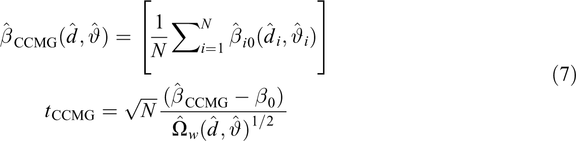
From the slope coefficients of the individual series, the common-correlation mean-group estimate for the panel can then be calculated as:

\begin{matrix} {\hat{β}}_{CCMG} (\hat{d}, \hat{ϑ}) = [\frac{1}{N} \sum_{i = 1}^{N} {\hat{β}}_{i 0} ({\hat{d}}_{i}, {\hat{ϑ}}_{i})] \\ t_{CCMG} = \sqrt{N} \frac{({\hat{β}}_{CCMG} - β_{0})}{{\hat{Ω}}_{w} {(\hat{d}, \hat{ϑ})}^{1 / 2}} \end{matrix}

where $\hat{d}, \hat{ϑ}$ are parameter vectors and $Ω_{w} (\hat{d}, \hat{ϑ})$ is an estimate of the asymptotic variance–covariance matrix, obtained nonparametrically based on the GLS slope estimates as:

{\hat{Ω}}_{w} (\hat{d}, \hat{ϑ}) = \frac{1}{N - 1} {\sum_{i = 1}^{N} ({\hat{β}}_{i 0} ({\hat{d}}_{i}, {\hat{ϑ}}_{i}) - {\hat{β}}_{CCMG} (\hat{d}, \hat{ϑ})) \times ({\hat{β}}_{i 0} ({\hat{d}}_{i}, {\hat{ϑ}}_{i}) - {\hat{β}}_{CCMG} (\hat{d}, \hat{ϑ}))}^{'}

Empirical analysis

Data

For the empirical analysis, we use quarterly data of the logarithm of international tourist arrivals and the logarithm of GDP for a sample of 14 European countries covering the period 1995–2019.⁴ Data of quarterly GDP are obtained from the Quarterly National Accounts elaborated by the OECD (2020) and refer to nominal GDP in US dollars. Data of quarterly tourist arrivals are obtained from Eurostat (2020) and refer to tourist arrivals in hotels, holiday and other short-stay accommodation, such as camping grounds. Both series are seasonally adjusted and expressed in logarithms. Figure 1 shows the evolution of both series. Both series feature an upward trend for all countries.

Figure 1.

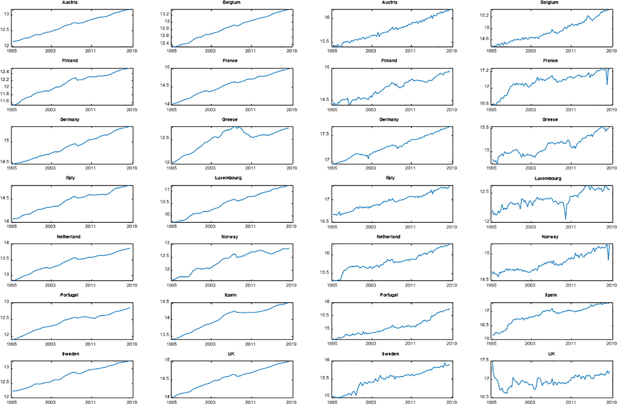
Real GDP and tourist arrivals in logs, 1995–2019: (a) (columns 1 and 2), (b) (columns 3 and 4).

Estimation results

In this section, we investigate the long-run relationship between GDP and tourist arrivals of 14 European countries. In a first step, we analyse the relationship with standard panel cointegration methods, and in a second step, we employ the fractional panel data method by Ergemen (2019). Moreover, taking into account that Perles-Ribes et al. (2017) and Pérez-Rodríguez et al. (2020) have shown that the global financial and economic crisis from 2007 to 2010 and the Arab spring potentially have weakened the long-run relationship between tourism and economic growth, we separately analyse two periods: first, the full sample (1995–2019) and, second, the sample prior to the global economic and financial crisis (up to the second quarter of 2007).

Standard panel cointegration analysis

Here, we perform a standard cointegration analysis for the period 1995–2019. This allows us to compare the results from the standard methodology with our results from applying fractional cointegration techniques.

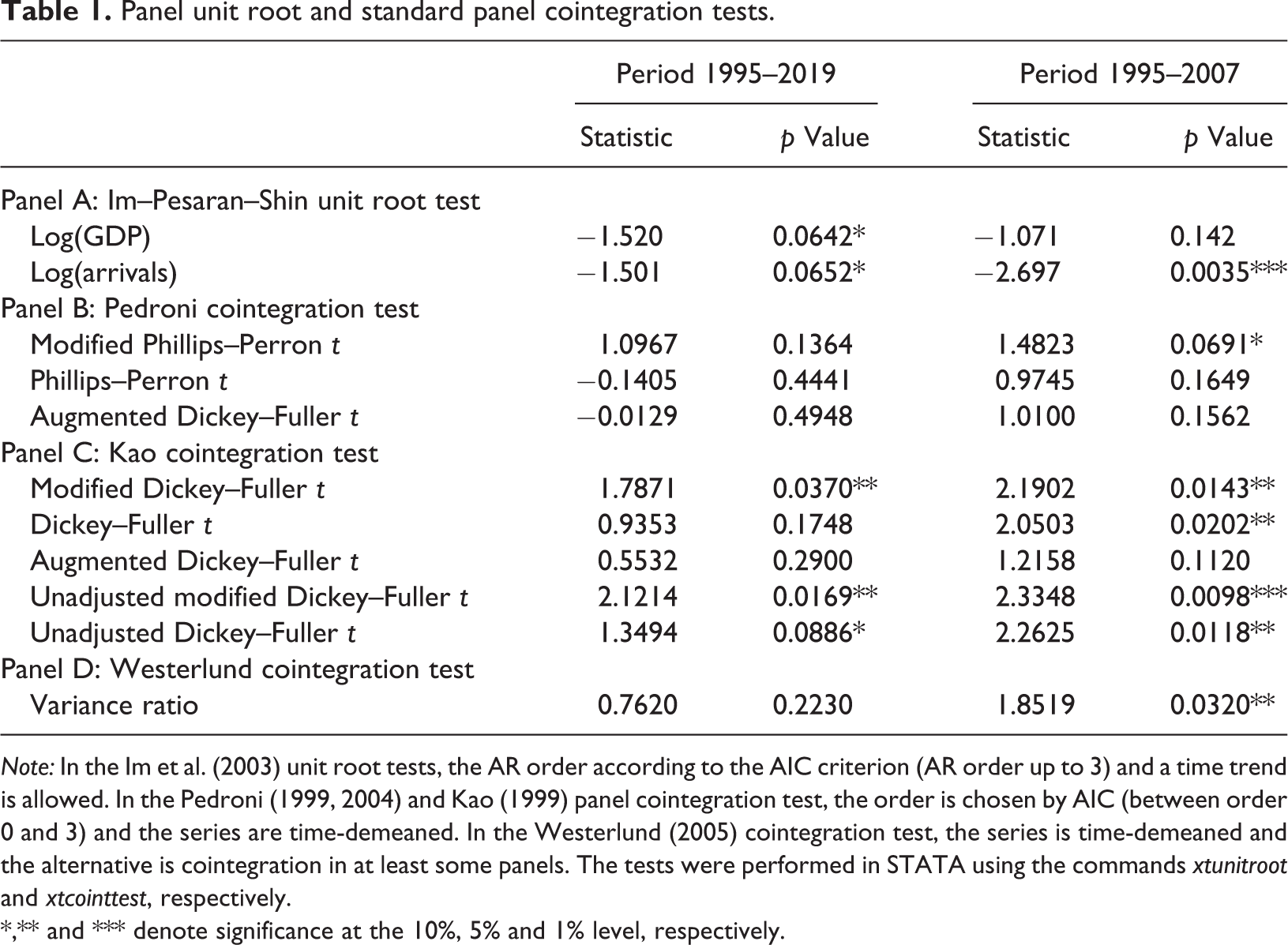
First, we perform Im et al. (2003) unit root tests (Table 1, panel A, left). The null hypothesis is a unit root in all panels and the alternative is that some panels are stationary, allowing for different coefficients for different panels. We choose the autoregressive (AR) order according to the akaike information criteria (AIC) criterion (AR order up to 3) and allow for a time trend. The null of unit roots is not rejected at the 5% level; p value of 0.0642 for log(GDP) and p value of 0.0652 for log(arrivals). Therefore, there is some evidence for unit roots in the series.

Table 1.

Panel unit root and standard panel cointegration tests.

	Period 1995–2019		Period 1995–2007
	Statistic	p Value	Statistic	p Value
Panel A: Im–Pesaran–Shin unit root test
Log(GDP)	−1.520	0.0642*	−1.071	0.142
Log(arrivals)	−1.501	0.0652*	−2.697	0.0035***
Panel B: Pedroni cointegration test
Modified Phillips–Perron t	1.0967	0.1364	1.4823	0.0691*
Phillips–Perron t	−0.1405	0.4441	0.9745	0.1649
Augmented Dickey–Fuller t	−0.0129	0.4948	1.0100	0.1562
Panel C: Kao cointegration test
Modified Dickey–Fuller t	1.7871	0.0370**	2.1902	0.0143**
Dickey–Fuller t	0.9353	0.1748	2.0503	0.0202**
Augmented Dickey–Fuller t	0.5532	0.2900	1.2158	0.1120
Unadjusted modified Dickey–Fuller t	2.1214	0.0169**	2.3348	0.0098***
Unadjusted Dickey–Fuller t	1.3494	0.0886*	2.2625	0.0118**
Panel D: Westerlund cointegration test
Variance ratio	0.7620	0.2230	1.8519	0.0320**

Note: In the Im et al. (2003) unit root tests, the AR order according to the AIC criterion (AR order up to 3) and a time trend is allowed. In the Pedroni (1999, 2004) and Kao (1999) panel cointegration test, the order is chosen by AIC (between order 0 and 3) and the series are time-demeaned. In the Westerlund (2005) cointegration test, the series is time-demeaned and the alternative is cointegration in at least some panels. The tests were performed in STATA using the commands xtunitroot and xtcointtest, respectively.

*,** and *** denote significance at the 10%, 5% and 1% level, respectively.

Second, Table 1 (panels B, C and D, left) presents results for three standard panel cointegration tests for the full sample and for the subsample prior to the crisis. We start with the Pedroni (1999, 2004) test for panel cointegration. In line with the previous literature, log(GDP) is the dependent variable and log(arrivals) is the potentially endogenous explanatory variable. We choose again the order according to the AIC criterion and correct for fixed effects by cross-section demeaning. Then, we perform the Kao (1999) and the Westerlund (2005) cointegration tests. The former proposes five test statistics based on the augmented dickey-fuller [(A)DF] regression.⁵ The latter imposes fewer restrictions with a different alternative hypothesis, namely that some but not necessarily all panels are cointegrated.⁶ For the full sample, only three of the five versions of the Kao cointegration test find evidence for cointegration.

We repeat the analysis for the sample 1995 to 2007, that is, prior to the global financial and economic crisis. First, the Im et al. (2003) unit root test rejects the null of a unit root in all panels (p value of 0.0035) for tourist arrivals but does not reject it for GDP (p value of 0.142) (Table 1, panel A, right). Second, in Table 1 (panels B, C and D, right), we also include the Pedroni (1999, 2004), Kao (1999) and Westerlund (2005) panel cointegration tests for the period prior to the crisis. Here, four of the five versions of the Kao cointegration test and the Westerlund cointegration test find cointegration at the 5% significance level and one of the three versions of the Pedroni cointegration test does so at the 10% level.

After having found some evidence for cointegration, we estimate the panel data DOLS model (Pedroni, 2001). Table 2 provides the individual slope coefficients obtained by dynamic OLS – with a linear trend in the cointegration relationship and two leads and lags of the differenced explanatory variable – together with the standard errors for both periods. First, for the overall period (Table 2, panel A), the slope coefficients are both positive and negative, varying quite widely. The slope coefficients are significantly negative for Belgium and Norway and significantly positive for France, Germany, Italy and Spain. The corresponding group-mean panel dynamic ordinary least squares estimator amounts to 0.10 with a t statistic of 3.53.⁷ The group mean therefore is rather low. Therefore, from the previous results, there is some evidence of cointegration, especially for European top tourist destinations such as France, Spain and Italy.

Table 2.

Individual DOLS estimation.

	Panel A: Period 1995–2019			Panel B: Period 1995–2007
Countries	${\hat{β}}_{i 0}$	$SE ({\hat{β}}_{i 0})$	t stat	${\hat{β}}_{i 0}$	$SE ({\hat{β}}_{i 0})$	t stat
Austria	0.01	0.21	0.06	0.45	0.38	1.21
Belgium	-0.26**	0.12	-2.26	0.53***	0.14	3.72
Finland	0.81	0.54	1.49	0.03	0.31	0.09
France	0.49***	0.09	5.51	0.31***	0.04	7.16
Germany	0.43***	0.12	3.55	0.09	0.12	0.77
Greece	-0.35	0.64	-0.55	-0.11***	0.03	-4.4
Italy	0.69*	0.39	1.77	0.7***	0.07	9.54
Luxembourg	0.05	0.13	0.36	0.39***	0.15	2.7
The Netherlands	0.21	0.24	0.86	0.26***	0.03	8.38
Norway	-1.22**	0.62	-1.96	0.74***	0.15	4.85
Portugal	-0.11	0.22	-0.5	0.49***	0.06	7.7
Spain	0.57***	0.13	4.39	-0.03	0.02	-1.52
Sweden	0.13	0.09	1.36	-0.23***	0.06	-3.99
UK	-0.09	0.1	-0.87	-0.01	0.01	-1.28

Note: DOLS: dynamic ordinary least squares. DOLS estimates with standard errors and t statistics. The regressions contain lags and leads of the differenced explanatory variable as chosen by AIC and a time trend in the cointegration relationship. The analysis was performed in STATA with the command xtcointreg.

*, ** and *** denote significance at the 10%, 5% and 1% level, respectively.

Table 2 (panel B) presents the individual slope estimates of the DOLS, again with time trends in the cointegration relationship and two leads and lags, for the sample prior to the crisis. The coefficients are significantly positive for Belgium, France, Italy, the Netherlands, Norway and Portugal and significantly negative for Greece and Sweden. The group-mean panel dynamic ordinary least squares estimator for the smaller sample with time demeaning and two lags and leads is 0.26 with a t statistic of 9.33. Thus, there is a somehow stronger relationship between tourism and economic growth prior to the crisis.

To conclude, evidence of cointegration between tourism and economic growth is found for a selected group of European countries. In particular, we found evidence for a long-run relationship between tourism and economic growth for the most important tourist destinations, that is, for France, Italy and Spain. Moreover, these are countries severely affected by the pandemic, so the tourism sector can play a relevant role in the recovery if proper actions are taken to ensure sanitary measures and the safety of tourists travelling to these destinations.

However, we also found that results for the whole sample and for the sample prior to the crisis differ, with a stronger relationship prior to the crisis. This result has been previously obtained in the empirical literature for the case of Spain in Perles-Ribes et al. (2017). These authors concluded that the cointegration relationship between tourism and economic growth has become less clear since the global financial and economic crisis and the Arab spring.

Yet, as discussed in the introduction, a standard panel cointegration setup might be too restrictive and a fractional one might lead to more accurate results. Therefore, in the next section, we employ the panel fractional cointegration method.

Fractional panel cointegration

In this section, we estimate the fractionally integrated heterogeneous panel data model.

First, we estimate the memory parameters for both series by Robinson (1995)’s local Whittle (LW) estimator for bandwidths of 0.6 and 0.7. Table 3 (panel A) presents that while the memory of log(GDP) is often above one, the one of log(arrivals) mostly is below one. For the sample before the crisis (Table 3, panel B), the estimates vary more widely, which is not surprising, given the rather short time series dimension, especially for a semiparametric method.

Table 3.

Local Whittle memory estimates of log(GDP) and log(arrivals).

b	Austria	Belgium	Finland	France	Germany	Greece	Italy	Luxembourg	The Netherlands	Norway	Portugal	Spain	Sweden	UK
Panel A: Period 1995–2019
(1) log(GDP)
0.6	0.8977	0.9084	1.3247	1.2857	0.944	1.4358	1.234	1.0977	1.3198	1.1766	1.3692	1.6693	1.0468	1.0085
0.7	1.4539	1.4038	1.3222	1.6585	1.2107	1.5531	1.522	1.4055	1.4912	1.5057	1.5686	1.7182	1.64	1.4214
(2) log(arrivals)
0.6	0.5466	0.8022	0.9896	0.966	1.1587	0.957	0.7448	0.6973	1.3431	0.7712	1.0017	1.3494	0.8768	1.0494
0.7	0.6462	0.915	0.8024	0.8905	1.1878	1.0066	0.7496	0.7537	1.0502	0.5811	0.9591	1.1956	0.6715	1.004
Panel B: Period 1995–2007
(1) log(GDP)
0.6	1.0481	1.4251	1.1626	1.6665	1.0404	0.9117	1.5685	1.3720	1.5068	1.6617	1.5716	1.6811	1.3333	0.7434
0.7	2.0352	2.4212	1.2937	2.0064	1.1397	1.4437	1.7463	1.3811	1.8317	1.7143	1.3652	2.2083	1.9046	1.6456
(2) log(arrivals)
0.6	0.0523	0.8487	0.7072	1.2833	1.3224	1.1052	0.6678	0.4381	1.1123	0.9663	0.6067	1.0053	0.5970	1.0552
0.7	0.1600	0.6168	0.7751	1.0662	1.0816	1.2029	0.6221	0.4735	1.1729	1.0338	0.8028	1.0675	0.5635	1.1423

Note: The semiparametric memory estimation by the local Whittle estimator (Robinson, 1995) was implemented in MATLAB using codes by Katsumi Shimotsu. Since consistency of this estimator requires d < 1, we estimate the memory for the first-differenced series and add 1 to the resulting estimate.

Second, we estimate the fractionally integrated heterogeneous panel data model. As aforementioned, the memory of the individual series depends on the memory of the factors and the memory of the individual defactored series. A common memory caused by the dependence on a persistent common factor can lead to spurious regressions (Ergemen and Velasco, 2017).

Therefore, we apply the methodology of Ergemen (2019) to the data set of log(GDP) and log(arrivals) of the 14 countries. By doing so, we can disentangle the long-run relationship of individual countries from the one of the factors. We correct for volatility characteristics of the two series. The methodology can accommodate up to two latent factors with potentially different memory parameters. The factors further can feature common deterministic trends. LW estimates of the factors are obtained from the memory estimates of the cross section averages for the two variables. In particular, the LW estimates are 1.13 and 1.04 for bandwidths 0.6 and 0.7, respectively, for log(arrivals) and 1.23 and 1.50 for log(GDP). The memory of the more persistent factor is therefore estimated as 1.23 or 1.50, depending on the bandwidth.

Table 4 presents the results for the fractionally integrated heterogeneous panel data cointegration model. Specifically, it contains the cointegration relationship ( ${\hat{β}}_{i 0}$ ) together with its standard errors, the memory of the defactored explanatory variable ( ${\hat{ϑ}}_{i 0}$ ), the residual integration order estimates ( ${\hat{d}}_{i 0}$ ) and the innovation correlation ${\hat{ρ}}_{i}$ . As aforementioned, non-trivial cointegration requires that ${\hat{d}}_{i 0}$ < ${\hat{ϑ}}_{i 0}$ which could be tested with a t test, $t = ({\hat{ϑ}}_{i 0} - {\hat{d}}_{i 0}) / SE ({\hat{ϑ}}_{i 0} - {\hat{d}}_{i 0})$ and that the estimated slope coefficients ${\hat{β}}_{i 0}$ are statistically significant. Since $SE ({\hat{ϑ}}_{i 0} - {\hat{d}}_{i 0})$ depends on $cov ({\hat{ϑ}}_{i 0}, {\hat{d}}_{i 0})$ , whose estimation is rather complicated, we compare instead the individual confidence intervals of ${\hat{ϑ}}_{i 0}$ and ${\hat{d}}_{i 0}$ and reject the null hypothesis of ${\hat{d}}_{i 0} \geq {\hat{ϑ}}_{i 0}$ if the confidence interval of ${\hat{d}}_{i 0}$ is strictly below the one of ${\hat{ϑ}}_{i 0}$ .⁸ Table 4 includes both confidence intervals at the 10% significance level, ${CI}_{ϑ_{i 0}}^{90 %}$ and ${CI}_{d_{i 0}}^{90 %}$ and indicates in bold the cases in which the confidence intervals are such that the null is rejected.

Table 4.

Estimation of the panel fractional cointegrated model.

	Austria	Belgium	Finland	France	Germany	Greece	Italy	Luxembourg	The Netherlands	Norway	Portugal	Spain	Sweden	UK
Panel A: Period 1995–2019
${\hat{β}}_{i 0}$	−0.0134***	0.0045***	−0.121***	0.0031**	−0.0821***	0.0056	−0.0016	0.0267***	−0.1494***	0.0147*	0.0265***	−0.0081***	−0.0163***	0.1791***
$SE ({\hat{β}}_{i 0})$	0.0017	0.0015	0.0027	0.0015	0.0027	0.0056	0.0021	0.0034	0.0017	0.0047	0.0025	0.0012	0.0026	0.0037
${\hat{ϑ}}_{i 0}$	0.5722***	0.8338***	0.7888***	0.6329***	0.7166***	0.8355***	0.6297***	0.7176**	0.9974***	0.5033**	0.8509***	0.8993***	0.6611***	0.9453**
$SE ({\hat{ϑ}}_{i 0})$	0.0883	0.0952	0.1187	0.2305	0.0641	0.169	0.1002	0.2956	0.0977	0.2591	0.0964	0.0911	0.1354	0.3866
${CI}_{ϑ_{i 0}}^{90 %}$	[0.43, 0.72]	[0.68, 0.99]	[0.59, 0.98]	[0.25, 1.01]	[0.61, 0.82]	[0.56, 1.11]	[0.47, 0.79]	[0.23, 1.2]	[0.84, 1.16]	[0.08, 0.93]	[0.69, 1.01]	[0.75, 1.05]	[0.44, 0.88]	[0.31, 1.58]
${\hat{d}}_{i 0}$	1.275***	0.47***	0.128***	0.545***	1.178***	1.5***	0.645***	0.001	1.154***	0.467***	0.702***	0.707***	1.09***	0.21***
$SE ({\hat{d}}_{i 0})$	0.016	0.0144	0.0263	0.0137	0.0239	0.0483	0.0191	0.0317	0.0159	0.0422	0.024	0.0115	0.0236	0.025
${CI}_{d_{i 0}}^{90 %}$	[1.25, 1.3]	[0.45, 0.49]	[0.08, 0.17]	[0.52, 0.57]	[1.14, 1.22]	[1.42, 1.58]	[0.61, 0.68]	[−0.05, 0.05]	[1.13, 1.18]	[0.4, 0.54]	[0.66, 0.74]	[0.69, 0.73]	[1.05, 1.13]	[0.17, 0.25]
${\hat{ρ}}_{i}$	0.0697	0.0036	0.2095	−0.0006	0.1812**	0.0044	0.0215	−0.0182	0.1868***	−0.006	0.1112	−0.0206	−0.0905	−0.3581*
Panel B: Period 1995–2007
${\hat{β}}_{i 0}$	−0.0079**	−0.0138***	−0.1704***	0.0296***	0.0696***	−0.0187***	−0.0231***	0.0283***	−0.3451***	0.0213**	0.0114**	0.4682***	−0.0419***	−0.0261***
$SE ({\hat{β}}_{i 0})$	0.0039	0.0038	0.0063	0.0038	0.0076	0.0068	0.0055	0.0089	0.0042	0.0108	0.0057	0.0025	0.006	0.0049
${\hat{ϑ}}_{i 0}$	0.4322**	0.829***	0.7415***	0.9872***	0.6395***	0.7632*	0.3683***	0.6273	1.0529***	0.779*	0.5915***	0.8628***	0.7098***	1.0555*
$SE ({\hat{ϑ}}_{i 0})$	0.2126	0.2205	0.2567	0.1566	0.1464	0.4024	0.1876	0.3854	0.1854	0.4041	0.2198	0.1162	0.2172	0.5529
${CI}_{ϑ_{i 0}}^{90 %}$	[0.08, 0.78]	[0.47, 1.19]	[0.32, 1.16]	[0.73, 1.24]	[0.4, 0.88]	[0.1, 1.42]	[0.06, 0.68]	[0, 1.26]	[0.75, 1.36]	[0.12, 1.44]	[0.23, 0.95]	[0.67, 1.05]	[0.35, 1.07]	[0.15, 1.96]
${\hat{d}}_{i 0}$	0.426***	0.404***	1.345***	0.682***	0.001	1.5***	0.567***	1.328***	1.188***	0.433***	0.881***	0.222***	1.477***	0.458***
$SE ({\hat{d}}_{i 0})$	0.0245	0.0236	0.0425	0.0223	0.0504	0.0419	0.0334	0.0561	0.0242	0.063	0.0367	0.0148	0.0395	0.0307
${CI}_{d_{i 0}}^{90 %}$	[0.39, 0.47]	[0.37, 0.44]	[1.28, 1.41]	[0.65, 0.72]	[−0.08, 0.08]	[1.43, 1.57]	[0.51, 0.62]	[1.24, 1.42]	[1.15, 1.23]	[0.33, 0.54]	[0.82, 0.94]	[0.2, 0.25]	[1.41, 1.54]	[0.41, 0.51]
${\hat{ρ}}_{i}$	0.0624	−0.0069	0.2499***	0.1951	−0.0566	−0.0064	−0.1072	−0.0261	0.4013*	0.1243	0.0727	−0.4964*	−0.2203	0.0099

Note: Estimates of the slope coefficient, of the memory of the defactored series, residual integration order (all with standard errors) and the innovation correlation estimates with *, ** and *** denoting significance at the 10%, 5% and 1% level, respectively. The estimation was performed in MATLAB using the original codes kindly provided by Emre Ergemen.

For the overall period (Table 4, panel A), three features stand out: first, the slope coefficients are rather small and, second and more strikingly, the ones of Finland and Spain are negative. Positive larger coefficients found elsewhere potentially might be due to the relationship between the underlying latent factors. Finally, results differ considerably from the ones in the previous section.

Similarly, as in the last section, we calculate the mean-group estimate for the panel. From formulas (7) and (8), ${\hat{β}}_{CCMG} (\hat{d}, \hat{ϑ}) = - 0.0035$ , which is very close to 0, with a standard error of 0.1105. Thus, the null of zero mean-group slopes cannot be rejected.

For the whole sample (Table 4, panel A), we find a nontrivial cointegration relationship (at the 10% level) only for Belgium, Luxembourg, and UK and for Finland and Spain (the latter both with a negative slope coefficient). For all these countries, except Luxembourg, the residual integration order is statistically larger than 0, thus shocks are persistent and reversion to the equilibrium is slow. Besides, for Germany, the Netherlands and UK, the innovations are correlated (statistical significance of ${\hat{ρ}}_{i}$ ), potentially due to country-specific feedback effects such as tourism-related governmental spending, after accounting for common correlations (such as OECD or European Union membership or being a high-income country). Therefore, contrary to what is obtained with standard cointegration methods (Table 2), fractional cointegration is mainly found for North European countries rather than for the Southern ones (which are the most important tourist destinations).

For the sample prior to the crisis (Table 4, panel B), Belgium features a significant negative relationship between tourism and economic growth and France, Germany and Spain feature significantly positive ones. For this sample, for Belgium, France and Spain, the residual integration order is statistically larger than 0, thus implying persistent shocks and slow reversion to the equilibrium. Finally, the mean-group estimate for the panel is −0.0043 with a standard error of 0.1825; therefore, it is statistically not distinguishable from 0.

To conclude, using panel cointegration methods, the case for a positive long-run relationship between tourism and economic growth is rather weak, with a slightly stronger one for the period prior to the 2007–2010 crisis. This confirms previous findings by Pérez-Rodríguez et al. (2020) and is in contrast to results using standard non-fractional methods. Therefore, the positive link between tourist arrivals and economic growth is weaker for this group of high-income countries, and a positive long-run nexus between tourism and economic growth more likely exists when the economies are not suffering crises episodes. Moreover, the evidence in favour of the TLGH is less clear for South European/Mediterranean countries, thus, confirming previous findings by Mello-Sampayo and Sousa-Vale (2012).

Conclusions

In this article, we have analysed the long-run GDP and inbound tourism relationship in a panel data framework, treating, in line with the empirical literature on TLGH, the former as the dependent variable and the latter as the endogenous explanatory variable. To account for country-specific differences, we have performed both a standard panel cointegration and a panel fractional cointegration analysis. For the latter, we have applied the fractionally heterogeneous integrated panel data system with individual stochastic components and cross-section dependence recently proposed by Ergemen (2019). It allows for a cointegrated system analysis in the defactored observed series and incorporates long-range dependence and short-memory dynamics and allows for deterministic time trends.

The empirical study is based on a sample of 14 European countries chosen due to the availability of sufficiently long series of tourist arrivals and GDP. More specifically, we use quarterly data from the fourth quarter of 1995 to the fourth quarter of 2019. We have estimated the relationship between log(GDP) and log(arrivals) using both standard panel cointegration model and panel fractionally cointegrated models, Pedroni (1999, 2001, 2004) and Ergemen (2019), respectively.

In both approaches, cointegration results differ for the whole sample and for the sample prior to the crisis, with a stronger relationship prior to the crisis. Especially, in the fractionally heterogeneous panel data model, the case for a positive long-run relationship between tourism and economic growth is rather weak, being slightly stronger for the period prior to this crisis. This confirms previous findings by Pérez-Rodríguez et al. (2020) and Perles-Ribes et al. (2017) that the validity of TLGH is less clear-cut during sample periods that include crisis episodes. Once enough data are available, it would be interesting to analyse the effect on the TLGH of the COVID-19 pandemic, which, as aforementioned, has heavily impacted the tourism sector.

Moreover, when panel fractional cointegration techniques are applied for the whole sample period, we find evidence in favour of the TLGH mainly for North European countries. This confirms findings by Mello-Sampayo and Sousa-Valle (2012) who obtained that tourism development has a higher impact on GDP in the North than in South. However, if we focus on the pre-crisis period, evidence in favour of the TLGH is also obtained for the relevant tourist destinations Spain and France. In addition, in most cases in which a long-run equilibrium exists, the reversion to it is rather slow due to the persistence of shocks. In consequence, the efficacy of tourism policies on economic growth is further reduced in the short term. Thus, it appears that the economic importance of tourism especially for touristic countries has reduced. Therefore, countries with an important tourism sector, such as Spain or France, should design strategic policies aimed at preventing any decrease in tourist arrivals during crises or periods of instability. It is noteworthy that neglecting this higher persistence can lead policymakers to wrongly assess shocks and therefore underestimate their effect on the economic cycle.

As aforementioned, tourism expenditures might have been the better proxy for the purpose of our analysis. In fact, this could be a reason why we found a larger impact of tourism on economic growth in North European rather than in South European/Mediterranean countries. That is, South European/Mediterranean countries, specialized in mass tourism, might be receiving a larger number of tourist arrivals but expenditure per capita might not necessary be larger. In consequence, they might need to raise tourist receipts if they want to stimulate economic growth, especially during crises episodes. Therefore, government and stakeholders need to design policies that aim not only at increasing inbound tourism but also at raising average spending per tourist. This issue becomes crucial if they want to minimize the impact of the pandemic in the long term.

However, the COVID-19 crisis has completely changed this scenario of continuous growth of international tourism. According to the World Tourism Organization (UNWTO) (2020), during the first quarter of 2020, there was a decrease in international tourism flows by 22% worldwide and by 19% in Europe. International tourist arrivals declined by around 60–80%, depending on containment measures, the duration of travel restrictions and re-opening of international borders. Consequently, the expected impact on countries’ economies is huge, putting at risk around 100–120 million of direct jobs in the tourism sector.

For the case of Europe, some of the most important tourist destinations, such as France, Italy or Spain, are also the most affected countries by this pandemic. These countries implemented severe lockdowns, and as a result, all of them experience dramatic GDP declines in 2020. Moreover, European countries are open economies with sectors which are highly sensitive to disruptions in the free movement of persons, such as the tourist industry, and with a high share of small businesses that are particularly vulnerable in this crisis. Indeed, travel and tourism were the first sectors hit by the pandemic and, probably, will be the last ones to resume their activities. Therefore, European countries which depend more on the tourism sector will suffer larger declines in their economic activity.

At the same time, having reliable data and applying appropriate econometric techniques become crucial not only to evaluate the impact of the COVID-19 crisis but also to design policy measures to minimize potential problems in the tourism sector. For this reason, more sophisticated and flexible econometric techniques to analyse the impact of tourism on economic growth are welcome in the debate about the magnitude of this unprecedented global crisis in the tourism sector. For all these reasons, a rigorous and in-depth analysis of the impact of the tourism sector on European GDP is needed for a proper quantification of the magnitude of this crisis. This could help policymakers and stakeholders in the tourism sector to design a recovery plan and to avoid a larger impact from a potential worsening of the pandemic.

As argued by Brida et al. (2016), it is widely accepted that the most adequate proxy of inbound tourism demand is tourism expenditure, normally expressed in terms of tourism receipts. Moreover, according to Rosselló-Nadal and He (2019), estimated tourism elasticities vary depending on whether tourist arrivals or tourism expenditures are used. Therefore, a limitation of the present article is that we do not have a large and homogenous data set on tourism receipts for the countries under analysis.

Finally, it would have been interesting to see differences between less homogenous countries by incorporating a larger number of countries, covering countries from all over the world. This would allow us to validate the TLGH for different groups of countries (classified by development level, regions or tourism specialization). However, for such an analysis of the TLGH, homogeneous data for a large sample of countries with a long sample period are unavailable.

Footnotes

Declaration of conflicting interests

The author(s) declared no potential conflicts of interest with respect to the research, authorship, and/or publication of this article.

Funding

The author(s) received no financial support for the research, authorship, and/or publication of this article.

ORCID iDs

Jorge V Pérez-Rodríguez

María Santana-Gallego

Notes

References

Antonakakis

Dragouni

Filis

(2015) Tourism and growth: the times they are a-changing. Annals of Tourism Research 50: 165–169.

Balaguer

Cantavella-Jordá

(2002) Tourism as a long-run economic growth factor: the Spanish case. Applied Economics 34(7): 877–884.

Balcilar

van Eyden

Inglesi-Lotz

, et al. (2014) Time-varying linkages between tourism receipts and economic growth in South Africa. Applied Economics 46: 4381–4398.

Brau

Lanza

Pigliaru

(2007) How fast are small tourism countries growing? Evidence from the data for 1980-2003. Tourism Economics 13: 603–613.

Brida

Lanzilotta

Pereyra

, et al. (2015) A nonlinear approach to the tourism-led growth hypothesis: the case of the MERCOSUR. Current Issues in Tourism 18: 647–666.

Brida

Cortés-Jiménez

Pulina

(2016) Has the tourism-led growth hypothesis been validated? A literature review. Current Issues in Tourism 19(5): 394–430.

Castro-Nuño

Molina-Toucedo

Pablo-Romero

(2013) Tourism and GDP: a meta-analysis of panel data studies. Journal of Travel Research 52(6): 745–758.

Chien-Chiang

Chun-Ping

(2008) Tourism development and economic growth: A closer look at panels. Tourism Management 29: 180–192.

Chudik

Pesaran

(2015) Common correlated effects estimation of heterogeneous dynamic panel data models with weakly exogenous regressors. Journal of Econometrics 188: 393–420.

10.

Comerio

Strozzi

(2019) Tourism and its economic impact: a literature review using bibliometric tools. Tourism Economics 25(1): 109–131.

11.

Cortés-Jiménez

(2008) Which type of tourism matters to the regional economic growth? The cases of Spain and Italy. International Journal of Tourism Research 10: 127–139.

12.

Dittman

(2000) Residual-based tests for fractional cointegration: a Monte Carlo study. Journal of Time Series Analysis 21: 615–647.

13.

Dritsakis

(2004) Tourism as a long-run economic growth factor: an empirical investigation for Greece using causality analysis. Tourism Economics 10: 305–316.

14.

Dritsakis

(2012) Tourism development and economic growth in seven Mediterranean countries: a panel data approach. Tourism Economics 18: 801–816.

15.

Durbarry

(2004) Tourism and economic growth: the case of Mauritius. Tourism Economics 10: 389–401.

16.

Engle

Granger

CWJ

(1987) Co-integration and error correction: representation, estimation, and testing. Econometrica 55: 251–276.

17.

Ergemen

(2019) System estimation of panel data models under long-range dependence. Journal of Business & Economic Statistics 37, 1: 13–26.

18.

Ergemen

Velasco

(2017) Estimation of fractionally integrated panels with fixed-effects and cross-section dependence. Journal of Econometrics 196: 248–258.

19.

Eugenio-Martín

Morales

Scarpa

(2004) Tourism and economic growth in Latin American countries: a panel data approach. Fondazione Eni Enrico Mattei Working Paper Series, Nota di Lavoro 26 .

20.

Eurostat (2020) Eurostat Data. Available at: https://ec.europa.eu/eurostat/data/database (accessed March 2020).

21.

Fayissa

Nsiah

Tadasse

(2008) Impact of tourism on economic growth and development in Africa. Tourism Economics 14: 807–818.

22.

Figini

Vici

(2010) Tourism and growth in a cross-section of countries. Tourism Economics 16: 789–805.

23.

Fischer

Gil-Alana

(2009) The nature of the relationship between international tourism and international trade: the case of German imports of Spanish wine. Applied Economics 41(11): 1345–1359.

24.

Gil-Alana

Hualde

(2009) Fractional integration and cointegration: an overview and an empirical application. In: Mills

Patterson

(eds) Palgrave Handbook of Econometrics. London: Palgrave Macmillan.

25.

Gil-Alana

Mudida

de Gracia

(2014) Persistence, long memory and seasonality in Kenyan tourism series. Annals of Tourism Research 46: 89–101.

26.

Harb

Bassil

(2020) Gravity analysis of tourism flows and the ‘multilateral resistance to tourism’. Current Issues in Tourism 23(6): 666–678.

27.

Hassler

Demetrescu

Tarcolea

(2011) Asymptotic normal tests for integration in panels with cross-dependent units. Advances in Statistical Analysis 95: 187–204.

28.

Holzner

(2011) Tourism and economic development: the beach disease? Tourism Management 32: 922–933.

29.

Pesaran

Shin

(2003) Testing for unit roots in heterogeneous panels. Journal of Econometrics 115: 53–74.

30.

Kao

(1999) Spurious regression and residual-based tests for cointegration in panel data. Journal of Econometrics 90: 1–44.

31.

Mark

Sul

(2003) Cointegration vector estimation by panel DOLS and long run money demand. Oxford Bulletin of Economics and Statistics 65: 655–680.

32.

Mello-Sampayo

Sousa-Vale

(2012) Tourism and growth in European countries: an application of likelihood-based panel cointegration. School of Economics and Management, Technical University Lisbon. Working Paper 17. https://bru.iscte-iul.pt/wp-content/uploads/working-papers/series-1/ercwp0510.pdf (accessed March 2020).

33.

Meo

Sabir

Arain

, et al. (2020) Water resources and tourism development in South Asia: an application of dynamic common correlated effect (DCCE) model. Environmental Science and Pollution Research 27: 19678–19687.

34.

Narayan

(2004) Economic impact of tourism on Fiji’s economy: empirical evidence from the computable general equilibrium model. Tourism Economics 10(4): 419–433.

35.

Narayan

Prasad

(2003) Does tourism granger causes economic growth in Fiji? Empirical Economics Letters 2(5): 199–208.

36.

Narayan

Prasad

, et al. (2010) Tourism and economic growth: a panel data analysis for Pacific Island countries. Tourism Economics 16: 169–183.

37.

Newey

West

(1987) A simple, positive semi-definite, heteroskedasticity and autocorrelation consistent covariance matrix. Econometrica 55: 703–708.

38.

Nunkoo

Seetanah

Jaffur

ZRK

, et al. (2019) Tourism and economic growth: a meta-regression analysis. Journal of Travel Research 59(3): 404–423.

39.

OECD (2020) Quarterly National Accounts OECD Statistics. Available at: https://stats.oecd.org/Index.aspx?DataSetCode=QNA (accessed February 2020).

40.

(2005) The contribution of tourism development to economic growth in the Korean economy. Tourism Management 26: 39–44.

41.

Pablo-Romero

Molina

(2013) Tourism and economic growth: a review of empirical literature. Tourism Management Perspectives 8: 28–41.

42.

Paramati

Alam

Chen

(2017) The effects of tourism on economic growth and CO2 emissions: a comparison between developed and developing economies. Journal of Travel Research 56(6): 712–724.

43.

Pedroni

(1999) Critical values for cointegration tests in heterogeneous panels with multiple regressors. Oxford Bulletin of Economics and Statistics 61: 653–670.

44.

Pedroni

(2001) Purchasing power parity tests in cointegrated panels. Review of Economics and Statistics 83: 727–731.

45.

Pedroni

(2004) Panel cointegration: asymptotic and finite sample properties of pooled time series tests with an application to the PPP hypothesis. Econometric Theory 20: 597–625.

46.

Pérez-Rodríguez

Ledesma-Rodríguez

Santana-Gallego

(2015) Testing dependence between GDP and tourism’s growth rates. Tourism Management 48: 268–282.

47.

Pérez-Rodríguez

Rachinger

Santana-Gallego

(2020) Testing the validity of the tourism-led growth hypothesis under long-range dependence. Current Issues in Tourism. Epub ahead of print 24 March 2020. DOI: 10.1080/13683500.2020.1744537.

48.

Perles-Ribes

Ramón-Rodríguez

Rubia

, et al. (2017) Is the tourism-led growth hypothesis valid after the global economic and financial crisis? The case of Spain 1957-2014. Tourism Management 61: 96–109.

49.

Pesaran

(2006) Estimation and inference in large heterogeneous panels with multifactor error structure. Econometrica 74: 967–1012.

50.

Pesaran

Shin

Smith

(1999) Pooled mean group estimation of dynamic heterogeneous panels. Journal of the American Statistical Association 94: 621–634.

51.

Phiri

(2016) Tourism and economic growth in South Africa: evidence from linear and nonlinear cointegration frameworks. Managing Global Transitions 14(1): 31–53.

52.

Robinson

Velasco

(2015) Efficient inference on fractionally integrated panel data models with fixed effects. Journal of Econometrics 185: 435–452.

53.

Robinson

(1995) Gaussian semiparametric estimation of long range dependence. Annals of Statistics 23: 1630–1661.

54.

Rosselló-Nadal

(2019) Tourist arrivals versus tourist expenditures in modelling tourism demand. Tourism Economics 26(8): 1311–1326.

55.

Saleh

Assaf

Ihalanayake

, et al. (2015) A panel cointegration analysis of the impact of tourism on economic growth: evidence from the Middle East region. International Journal of Tourism Research 17: 209–220.

56.

Salifou

Haq

(2017) Tourism, globalization and economic growth: a panel cointegration analysis for selected West African States. Current Issues in Tourism 20(6): 664–667.

57.

Santana-Gallego

Ledesma-Rodríguez

Pérez-Rodríguez

(2011) Tourism and trade in OECD countries. A dynamic heterogeneous panel data analysis. Empirical Economics 41(2): 533.

58.

Seetenah

(2011) Assessing the dynamic economic impact of tourism for island economies. Annals of Tourism Research 38: 291–308.

59.

Sequeira

Nunes

(2008) Does tourism influence economic growth? A dynamic panel data approach. Applied Economics 40: 2431–2441.

60.

Shahzad

SJH

Shahbaz

Ferrer

(2017) Tourism-led growth hypothesis in the top ten tourist destinations: new evidence using the quantile-on-quantile approach. Tourism Management 60: 223–232.

61.

Tang

Tan

(2018) Tourism-led growth hypothesis: a new global evidence. Cornell Hospitality Quarterly 59(3): 304–311.

62.

UNWTO (2020) UNWTO World Tourism Barometer. May 2020. Available at: https://0-doi-org.llull.uib.es/10.18111/wtobarometereng (accessed June 2020).

63.

Wang

(2012) Threshold effects on development of tourism and economic growth. Tourism Economics 18: 1135–1141.

64.

Westerlund

(2005) New simple tests for panel cointegration. Econometric Reviews 24: 297–316.