Air transport capacity and tourism demand: A panel cointegration approach with cross-sectionally augmented autoregressive distributed lag (CS-ARDL) model

Abstract

This research aims to quantify the effect of air transport capacity on tourism demand by examining their long-term (cointegrating) relationship, accounting for cross-sectional dependence and endogeneity. Panel time series data from 2008Q1 to 2019Q4 for international tourist arrivals from 16 main origins to six Australian states are investigated. The study finds 1% increase in Available-Seat-Kilometers, seat capacity, or flight frequency can result in 0.4%–0.7% increase in tourist arrivals to Australia, adding to the body of evidence that shows a non-negligible aviation-led generative effect on tourism demand. The study finds ignoring cross-sectional dependence can result in significantly different, and potentially incorrect, coefficient estimates. Although using pre-COVID data, the results are useful in highlighting the likely aviation supply—tourism demand relations under reasonably well-performing market conditions. For greater tourism demand, findings call for more liberal international air services agreements, and direct/indirect air route development subsidies with minimum commitment of several years.

Keywords

air transport capacity tourism demand cointegration autoregressive distributed lag model panel time series cross-sectional dependence Australia

Introduction

Australia is a geographically remote tourism destination with a liberalized aviation market and a highly developed aviation – tourism ecosystem (Spasojevic and Lohmann, 2022). In 2019, the total nonstop air transport capacity (hereafter air transport capacity) to Australia increased by more than 60% compared to 10 years before (from 16.5 to 26.8 million seats) (Cirium, 2021). Within the same period, the total number of international tourist arrivals (TA) to Australia almost doubled (from 5.56 to 9.47 million) (Australian Bureau of Statistics, 2021). These two observations do not happen in coincidence but stem from intertwined interdependences between the air transport and tourism industries in the long term (Ivanova, 2017). For air transport-reliant destinations like Australia, guiding aviation policy and marketing designed for promoting tourism development relies on accurate yet robust estimates of the causal effect of air transport capacity (ATC) on tourism demand; for instance, destination marketing organizations such as Destination New South Wales in Australia use return-on-investment ratios for assessing air route development funds.

The causal effect of air transport capacity on tourism demand has a theoretical basis. Many tourism demand studies tend to be based on neoclassical consumer theory (Lim, 1997b, 1999). From their perspective, air transport capacity is a surrogate of the generalized cost of air transport borne by tourists. Air transport is one of the top three determinants in tourism demand modeling, in addition to tourists’ income and (destination) tourism prices (Lim, 1997b, 1999). Another theoretical motivation for considering the effect of air transport on tourism demand is based on gravity theory, which has a distance parameter. In this regard, air transport capacity is associated with the “distance” between the origin and destination, which in tourism parlance is defined as a measure of accessibility or connectivity for the destination. Empirical evidence from meta-analyses has demonstrated that the omission of the transport factor results in larger size coefficient estimates of tourism price elasticity (Peng et al., 2015) and income elasticity (Gallet and Doucouliagos, 2014).

However, modeling the causal effect of air transport capacity on tourism demand needs to resolve at least two challenges. First, the commonly recognized bidirectional causality (aka the classic “chicken or egg” dilemma by Koo et al. (2017)) must be appropriately disentangled. In the econometric context, this bidirectional causality results in a correlation between the explanatory variable and residuals (aka the endogeneity problem); thus, the estimates will be inconsistent. The endogeneity problem can be mitigated by introducing instrumental variables (hereafter instruments) in the empirical models (e.g., Alderighi and Gaggero, 2019; Koo et al., 2017; Tsui, 2017). Second, the scale of data used should not be too limited and the model specifications (i.e., explanatory variables included, econometric techniques used) must adequately deal with the structure of the data (Fuleky et al., 2014). Several empirical studies on the air transport capacity – tourism demand nexus have been undertaken in the last decade, particularly in the Asia Pacific region (e.g., Koo et al., 2013; Koo et al., 2017; Koo et al., 2018; Tsui, 2017; Tsui et al., 2019; Salesi et al., 2021). However, these studies have been dominated by either small $N$ or small $T$ panel data. To the best of authors’ knowledge, a wide range of elasticity estimates is also observed among these studies, even for the same destination, resulting in relatively imprecise recommendation for managerial action and policy; for instance, in the evaluation of return-on-investment in air route development explained earlier. To generate robust empirical estimates, the abovementioned two challenges must be adequately addressed.

Against this background, the aim of the study is to quantify the causal effect of air transport capacity on Australian inbound tourism demand using large-scale panel data with 48 origin-destination (O-D) pairs during 2008Q1-2019Q4 ( $N = 48$ , $T = 48$ ) (aka panel time series). A large-scale panel dataset enables a parsimonious model specification to obtain a high degree of freedom, which increases the efficiency and stability of the coefficient estimates (Gunter et al., 2019). In achieving the above aim, we overcome the afore mentioned two challenges by employing a Cross-Sectionally Augmented Autoregressive Distributed Lag (CS-ARDL) model in error-correction form, developed by Chudik and Pesaran (2015). The application of this method overcomes the endogeneity issue with instruments (using Herfindahl–Hirschman Index or HHI), while the second issue pertaining to large panel is approached by accounting for the cross-sectional dependence. In the tourism economics context, cross-sectional dependence arises from the fact that tourists flowing from different origins to a particular destination may be affected by many common factors (e.g., outbreaks of disasters/crises), which can lead to a common pattern of tourist flows across origins (Morley et al., 2014). Other sources of cross-sectional dependence could be economic policy uncertainties in a large country such as China, which is a major trading partner for many countries (Kuok et al., 2023).

Literature review

Tourism researchers have attempted to estimate the causal effect of air transport capacity on the tourism demand of a destination (see Table 1). These studies report a multitude of coefficient estimates concerning air transport capacity for different destinations. In their empirical models, a dummy variable is used to represent either (i) the launch of low-cost carrier (LCC) air services or (ii) the launch of nonstop flights (e.g., Chung and Whang, 2011; Duval and Schiff, 2011; Rey et al., 2011). While these studies have obtained significant positive coefficients of the air transport dummy variables, the approach adopted does not produce elasticity estimates.

Table 1.

Extant literature in air transport capacity and tourism demand.

Author(s)	Region(s)	Period	Data	Model	Variables (excl. controlling var.)	Findings
Tveteras and Roll (2014)	From 75 countries to Peru	2004–2009	N = 75; T = 6 (annual)	OLS	Tourist arrivals, flight frequency	1% increase in nonstop flights leads to 0.067% (0.32%) increase in tourist arrivals in the short (long) term.
Koo et al. (2017)	Between 14 main origins globally and 8 Australian states	2007, 2013	N = 112; T = 2 (annual)	IV-LIML	Tourist arrivals, resident departure, flight frequency	1% increase in direct air services leads to 0.23% increase in outbound tourism demand of Australia, but no significant effect is found on inbound tourism demand.
Tsui (2017)	Five New Zealand regions	2009M6-2015M7	N = 5; T = 74 (monthly)	IV-2SLS	Guest nights, LCC ASK	The LCCs’ ASK elasticity estimates of domestic guest nights range between 0.05%–0.85%.
Koo et al. (2018)	Tourist arrivals from 12 Asian origins to the eight Australian states	2005–2016	N = 96; T = 12 (annual)	GMM	Tourist arrivals, seat capacity	An annual increase in seat capacity by 100,000 (translated into an A380 flight every second day) results in 0.352% increase in inbound tourist arrivals.
Alderighi and Gaggero (2019)	From 24 European countries to 20 Italian regions	1999–2010	N = 480; T = 24 (semi-annual)	IV-ZINB	Tourist arrivals, flight frequency	An additional LCC flight can generate 74 tourist arrivals and 248 overnight tourists. An additional full-service flight reduces 29 tourist arrivals and 97 overnight tourists.
Balli et al. (2019)	From eight countries to New Zealand	1998M4-2015M7	N = 8; T = 207 (monthly)	VAR	Tourist arrivals, seat capacity	Airline seat capacity leads to more tourist arrivals from some countries but not for richer economies like Japan and US.
Tsui et al. (2019)	Six New Zealand regions	2008M1-2014M12	N = 6; T = 84 (monthly)	IV-3SLS	Tourist arrivals, ASK	1% increase in total ASK (FSC and LCC) leads to 0.065% increase in total (international and domestic) tourist arrivals.
Salesi et al. (2021)	From Australia and New Zealand to the four South Pacific countries	2008M1-2018M12	N = 8; T = 132 (monthly)	2SLS	Tourist arrivals, ASK	1% increase in ASK leads to 0.252%–0.797% increase in inbound tourists from Australia and New Zealand to the four South Pacific countries.
Mazzola et al. (2022)	13 island countries in the southern Europe	2000–2017	N = 13; T = 18 (annal)	OLS	Tourist arrivals, tourist, aircraft arrivals	1% increase in air transport supply leads to nearly 0.3% increase in tourist arrivals to the island countries in the southern Europe.

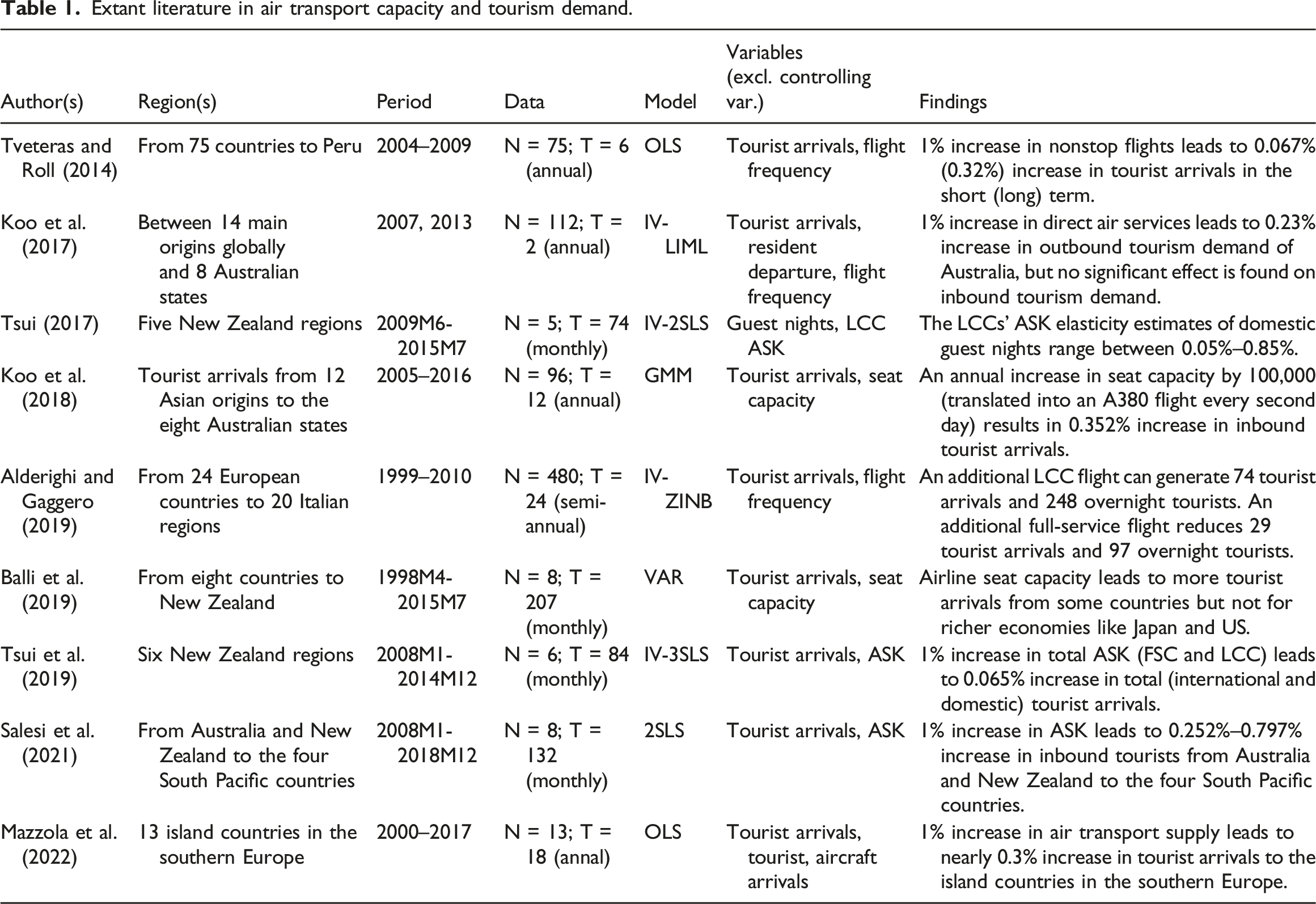
In other studies, quantitative measures of air transport capacity are used, such as flight frequency (e.g., Alderighi and Gaggero, 2019; Koo et al., 2017; Tveteras and Roll, 2014), total number of seats available (aka seat capacity) (e.g., Koo et al., 2013; Koo et al., 2018), and Available-Seat-Kilometers (ASK, a standardized unit of measure of capacity in airline management) (e.g., Tsui, 2017; Tsui et al., 2019; Salesi et al., 2021). From the perspective of tourists, the level of air transport capacity determines how convenient the tourists can choose a flight with a departure time as close to their most desired departure time, and this is referred to as schedule delay (Douglas and Miller, 1974). Furthermore, increased air transport capacity is also associated with lower airfare. According to Cattaneo et al. (2018), the negative relationship between air transport capacity and airfare can be explained in two ways. First, airline industry structures are usually oligopolistic; in the presence of more frequent services, competing airlines may have to reduce airfare to attract more travelers. Second, the economies of density, credited to lower average cost per passenger, also result in lower airfare.

As shown in Table 1, studies vary significantly in their samples and panel data characteristics. For example, Tsui (2017) investigates five New Zealand regions and finds that 1% increase in LCCs’ ASK results in 0.05%–0.85% increase in domestic guest nights. Tsui et al. (2019) focus on six main airports in New Zealand and find that 1% increase in total ASK (FSC and LCC) leads to 0.065% increase in total (international and domestic) tourist arrivals. However, the abovementioned studies do not differentiate between tourism origins. In other words, they implicitly assume the consumer utility functions are identical across all the origin countries, although segmentation by origins is desirable on theoretical grounds (Morley et al., 2014). Also, empirically, meta-analyses have given evidence that tourism demand elasticities differ across the origins of a common destination (e.g., Crouch, 1995; Lim, 1999; Peng et al., 2014; Peng et al., 2015).

Some studies differentiate the tourism-generating markets of a destination. For example, Koo et al. (2013) independently examine the Japan-Australia pair and China-Australia pair, and find that air passengers from Japan to Australia make quicker adjustments to changes in seat capacity than those from China to Australia. However, the authors focus on a small number of origin-destination pairs/routes, which limits the generalizability of the study. Other attempts examine the tourist flows for many O-D pairs/routes through a panel dataset. For example, Koo et al. (2017) use 112 O-D pairs, and they find a significant positive relationship between direct air services and the outbound tourism demand of Australia. Koo et al. (2018) reexamine Australia with a different panel dataset comprising O-D pairs between 12 Asian origins and the eight Australian states. The authors find a significant, albeit small effect of direct air services on tourist arrivals to Australia, which is equivalent to 0.352% increase in tourist arrivals for an annual rise of seat capacity by 100,000 (translated into an A380 flight every second day). However, the temporal observations of the panel data in these studies tend to be relatively limited, probably due to the increasing data requirement for a large sample of O-D pairs/routes. As seen above, previous studies have been limited to either small $N$ or small $T$ panel data, which cause large variations in coefficient estimates of air transport capacity; thus, the reliability of the practical implications generated may be questionable (Fuleky et al., 2014).

Methodology

With improvement in data collection technology, large $N$ large $T$ panel data are available for researchers to investigate the air transport capacity – tourism demand relations on many O-D pairs and longer time periods. However, unlike the widely available large $N$ small $T$ panel data (aka short panel), large $N$ large $T$ panel data is essentially a panel of time series (aka panel time series), which must be taken into account when selecting the appropriate econometric approach.

Panel cointegration

Invariably, time series of many economic variables are nonstationary, leading to spurious static OLS regression (Kao, 1999). However, simply differencing the nonstationary variables (to obtain stationary variables) eliminates some relevant information on the long-term properties of the underlying variables. Thus, the regression model on the relationship between different variables and the estimated coefficients may not be supported by rigorous theoretical reasoning. Engle and Granger (1987) argue that a linear combination of the studied variables may form a stationary process. Hence, such a linear combination indicates the long-term relationship (aka cointegrating relationship) between the studied variables.

Cointegration analysis is a suitable starting point when examining panel time series and it enables us to explore the long-term properties between air transport capacity and tourism demand. According to Granger (1986), economic theory is often based on the belief that certain pairs of economic variables do not significantly diverge from one another in the long term. Such variables may drift apart in the short term (e.g., one-off shock), but if they continue to deviate from the long-term steady relationship, some economic forces (e.g., market mechanism) will drive them back together. In the aviation industry, capacity decisions which involve fleet acquisition and flight crew training, must be planned on a long-term basis, at least several years ahead. Therefore, knowing the cointegrating relationship between air transport capacity and tourism demand is useful for developing aviation policy and marketing. The long-term steady relationship between air transport capacity and tourism demand can be modeled with the aid of an error correction specification, through which the long-term (cointegrating) relationship, short-term divergences, as well as the speed of convergence to the long-term relationship are separated. Cointegration analysis has received particular attention from economists and has been considered in policymaking related to major economic variables (i.e., consumption, employment, government expenditure, interest rate, investment, tax) (Granger, 2004). In addition, the superiority of imposing cointegrating restrictions in a forecasting system to improve the forecasting performance is a known practice by economists (e.g., Christoffersen and Diebold, 1997; Clements and Hendry, 1995) and tourism researchers (e.g., Kulendran and Witt, 2001; Li et al., 2006).

One commonly used cointegration technique is the Autoregressive Distributed Lag (ARDL) model. This model enables researchers to determine the cointegrating relationship between the studied variables through an error correction specification. The ARDL model is particularly suitable for cointegration analysis on panel time series for several reasons. First, the ARDL model allows for slope heterogeneity across sections. A widely used technique in examining short panel is to pool the data by imposing a common slope (e.g., fixed/random effects). However, such a technique generates inconsistent estimates in a dynamic model specification for panel time series because ignoring slope heterogeneity induces serial correlation in residuals (Pesaran and Smith, 1995). Unlike the conventional panel data technique, the ARDL model is estimated by (i) the mean group (MG) estimator (Pesaran and Smith, 1995) or (ii) the pooled mean group (PMG) estimator (Pesaran et al., 1999). In essence, the MG and PMG estimators estimate the section-specific equations independently; thus, the slope coefficients can be heterogenous. Second, the estimates generated by the ARDL model are valid regardless of whether the regressors are $I (0)$ (stationary), $I (1)$ (nonstationary), or a mixture of $I (0)$ and $I (1$ ) (Pesaran et al., 2001). In many cases, it is not easy to determine the stationarity of the underlying variables owing to the lack of power of the unit root tests used. Therefore, the ARDL model has an advantage over other cointegration techniques, which do not allow for a mixture of $I (0)$ and $I (1)$ regressors (e.g., fully modified ordinary least square (FMOLS), vector autoregression (VAR)).

Cross-sectional dependence

Another important econometric issue to be considered is cross-sectional dependence arising from the fact that the cross-sectional units are influenced by some omitted unobserved common factors (Frees, 1995). Unless the analysis of air transport capacity and tourism demand interaction is confined to a single origin-destination pair case study, it is likely cross-sectional dependence will be present in the data because the sample of interests will involve tourist flows from various origins to a destination. For panel data with small $T$ , it is typically assumed that the residuals of the regressions are cross-sectionally independent. However, when examining panel data with large $T$ , the problem of cross-sectional dependence in residuals will lead to inconsistent estimates and should be modeled (Pesaran, 2021).

The commonly correlated effects (CCE) estimator, proposed by Pesaran (2006), can mitigate the effect of cross-sectional dependence. The CCE estimator is a vector of cross-sectional averages of the studied variables incorporated as regressors and used to capture the unobserved common factors. It is robust to different types of cross-sectional dependence, potential unit roots in factors, and slope heterogeneity (Chudik and Pesaran, 2015). Based on Fuleky et al. (2014), the CCE estimator (i) is simple to implement; (ii) has good finite sample properties; (iii) does not require ex-ante information about the unobserved common factors; and (iv) offers good finite sample properties. The authors further show that when the empirical model is estimated by the FMOLS estimator, the price elasticity has the wrong (or positive) sign. However, the obtained price elasticity estimate is significant negative under the CCE estimator. Other tourism studies also report that the underlying coefficient estimates generated by the CCE estimator differ from those that do not correct for the cross-sectional dependence (e.g., Demir et al., 2020; Ghosh, 2022; Lee et al., 2021). To verify whether the residuals of the regression are cross-sectionally independent. The Pesaran (2021) test (aka the CD test) is conducted, which is based on the average pair-wise correlation coefficients of the individual regressions’ residuals.

CS-ARDL model

In this study, we employ the CS-ARDL model developed by Chudik and Pesaran (2015), which takes into account slope heterogeneity and cross-sectional dependence, to conduct a panel cointegration analysis on the air transport capacity – tourism demand nexus. Based on Chudik and Pesaran (2015), the CS-ARDL model is derived as follows. We assume the $A R D L (p, q)$ with p lagged orders of $y_{i t}$ and q lagged orders of $x_{i t}$ is given as:

y_{i t} = α_{i} + \sum_{j = 1}^{p} {η_{i j} y}_{i, t - j} + \sum_{k = 0}^{q} {β_{i k} x}_{i, t - k} + u_{i t}

(1)

And the

A R D L (p, q)

in error correction form is reparametrized as:

{Δ y}_{i t} = α_{i} + ϕ_{i} (y_{i, t - 1} - Ψ_{i} x_{i, t - 1}) + \sum_{j = 1}^{p - 1} η_{i j}^{*} {Δ y}_{i, t - j} + \sum_{k = 0}^{q - 1} β_{i k}^{*} {Δ x}_{i, t - k} + u_{i t}

(2)

where

$(y_{i, t - 1} - Ψ_{i} x_{i, t - 1}$ ) represents the long-term cointegrating relationship,

$ϕ_{i} = - (1 - \sum_{j = 1}^{p} η_{i j})$ denotes the error correction coefficient or speed of adjustment, $Ψ_{i} = ϕ_{i}^{- 1} \sum_{k = 0}^{q} β_{i k}$ is a vector of long-term coefficients,

$η_{i j}^{*} = - \sum_{m = j + 1}^{p} η_{i m}$ , for $j = 1, 2, \dots, p - 1$ , depicts the short-term coefficients of the dependent variables,

$β_{i k}^{*} = - \sum_{v = k + 1}^{q} β_{i v}$ , for $k = 0, 1, 2, \dots, q - 1$ , depicts the short-term coefficients of the explanatory variables.

We further decompose the residuals $u_{i t}$ into the unobserved common factors, $f_{t}$ , and their corresponding factor loadings, $λ$ (given by equation (3)). The independently and identically distributed (i.i.d.) residuals across the temporal and cross-sectional dimensions are denoted as $ε_{i t}$ . The unobserved common factors have different magnitudes of influences on the cross-sections determined by the corresponding factor loadings. As shown in equation (4), we assume that the unobserved common factors, $f_{t}$ , along with the lagged dependent variable, $y_{i, t - 1}$ , have feedback effects on the explanatory variables, $x_{i t}$ .

u_{i t} = γ_{i} f_{t} + ε_{i t},

(3)

x_{i t} = a_{i} + b_{i} y_{i, t - 1} + λ_{i} f_{t} + v_{i, t} .

(4)

Acting as proxies for the unobserved common factors, the cross-sectional averages of the dependent and explanatory variables, $\bar{y_{t - j}} = N^{- 1} \sum_{i = 1}^{N} y_{i, t - j}$ and $\bar{x_{t - k}} = N^{- 1} \sum_{k = 1}^{N} x_{i, t - k}$ , are plugged into Equation (1) as follows:

{\bar{y}}_{t} = \bar{α} + \sum_{j = 1}^{p} {\bar{η}}_{j} {\bar{y}}_{t - j} + \sum_{k = 0}^{q} {\bar{β}}_{k} \bar{x}_{t - k} + {\bar{Υ} f}_{t} + \bar{ε} .

(5)

Since the residuals,

ε_{i t}

, are i.i.d, we have

\bar{ε} = 0

. Hence, Eq. (5) can be transformed into:

f_{t} = ({\bar{y}}_{t} - \bar{α} - \sum_{j = 1}^{p} {\bar{η}}_{j} {\bar{y}}_{t - j} - \sum_{k = 0}^{q} {\bar{β}}_{k} {\bar{x}}_{t - k}) / \bar{Υ} .

(6)

Then, we plug equation (6) into equation (1) and obtain equation (7) as:

y_{i t} = α_{i} + \sum_{j = 1}^{p} {η_{i j} y}_{i, t - j} + \sum_{k = 0}^{q} {β_{i k} x}_{i, t - k} + \sum_{l = 0}^{s} ω_{i l} {\bar{z}}_{t - l} + ε_{i t},

(7)

where

{\bar{z}}_{t - l} = {({\bar{y}}_{t - l}, {\bar{x}}_{t - l})}^{'}

and

ω_{i l}

is the matrix of the coefficients of

{\bar{z}}_{t}

Likewise, the $C S - A R D L (p, q)$ model in error correction form is written as:

{Δ y}_{i t} = α_{i} + ϕ_{i} (y_{i, t - 1} - Ψ_{i} x_{i, t - 1}) + \sum_{j = 1}^{p - 1} {η_{i j}^{*} Δ y}_{i, t - j} + \sum_{k = 0}^{q - 1} {β_{i k}^{*} Δ x}_{i, t - k} + \sum_{l = 0}^{s} ω_{i l} {\bar{z}}_{t - l} + ε_{i t} .

(8)

The $C S - A R D L (p, q)$ model is estimated by the MG estimator or the PMG estimator. The MG estimator treats each of the individual sections separately, and the coefficients for the panel data are the averages of the corresponding coefficients across the sections. However, the MG estimator does not consider that some coefficients across sections may be similar, leading to inefficient estimates. The PMG estimator assumes that the long-term relationships are homogenous across sections while the intercepts, error correction coefficients, short-term coefficients, and residuals are allowed to differ across sections. If the assumption of homogeneity in long-term coefficients holds, the PMG generates more efficient estimates than the MG (Pesaran et al., 1999). We employ the Hausman (1978) specification test to determine the validity of the estimates generated by the PMG. Essentially, the Hausman (1978) test evaluates a consistent estimator, with an alternative estimator assumed to be more efficient under the assumption being tested. The null hypothesis indicates that there is no systematic difference between the two estimators; thus, the alternative estimator is more consistent and efficient. Conversely, if a systematic difference exists between the two estimators, we will suspect that the assumption being tested is invalid.

Variables and data

Subject to the availability of nonstop flights, we focus on quarterly O-D pair data (2008Q1-2019Q4) from 16 oversea markets worldwide to the six Australian states (New South Wales (NSW), Northern Territory (NT), Queensland (QLD), South Australia (SA), Victoria (VIC), and Western Australia (WA)). Our panel time series dataset comprises 48 time periods and 48 O-D pairs (or sections). The 16 origin markets are Canada, China, Fiji, Hong Kong, Indonesia, Japan, Malaysia, New Zealand, Papua New Guinea, Philippines, Singapore, South Korea, Taiwan, Thailand, USA, and Vietnam. The tourist flows of these 48 O-D pairs are likely to follow some common patterns because they belong to a single country (Shafiullah et al., 2019). The cointegrating relationship between the studied variables is given as $T A = f (A T C, Y, R E X)$ . This indicates that the number of tourist arrivals is a function of air transport capacity, income of tourists’ origin market (Y), and tourism prices proxied by real exchange rate (REX).

Numbers of short-term (less than one year) tourist arrivals are retrieved from the Department of Home Affairs (Australian Government). We also independently examine tourists for business, holiday, and visiting-friends-and-relatives (VFR). Data for air transport capacity, measured by Available-Seat-Kilometers (ASK), seat capacity, and flight frequency, are retrieved from the Cirium database. These three measures are used separately to enhance the robustness of our empirical results. Since the data are specified by airline and airport-airport pair, we need to make summations to generate the series for the O-D (origin market-Australian state) pairs to fit with the data for tourist arrivals to Australia as follows:

{A T C}_{i t} = \sum_{h = 1}^{c_{i}} \sum_{p = 1}^{d_{h}} {A T C}_{i h p t},

(9)

where

i

h

p

, and

t

denote the O-D pair, route (airport-airport pair), airline, and time period, respectively. The

c_{i}

and

d_{h}

indicate the total number of routes in O-D pair

i

and total number of airlines in route

h

, respectively. Importantly, we only consider over-the-coast nonstop flights to avoid double counting in case connecting flights exist. Over-the-coast flights are the legs of flights from the last oversea cities to the first Australian cities.

To correct for the endogeneity problem in our empirical model, we utilize the Herfindahl-Hirschman Index (HHI) as an instrument. A valid instrument must have causal effect on the endogenous explanatory variable but cannot directly affect the dependent variable (Greene, 2003). The HHI is a measure of market structure and is used as an instrument in the estimation of empirical models for the air transport capacity – tourism demand relations (e.g., Alsumairi and Tsui, 2017; Tsui, 2017; Salesi et al., 2021). This is because airlines’ decisions on capacity are heavily influenced by market structure (Mohammadian et al., 2019; Pitfield et al., 2010), whereas the market structure per se is believed to have no direct effect on demand for tourism.

The HHI is calculated by summing the squares of the percentage market share of each of the airlines competing in the same O-D pairs. In our study, the HHI is calculated as follows:

{H H I}_{i t} = \sum_{h = 1}^{s_{i}} {(\frac{{A S K}_{i h t}}{{A S K}_{i t}})}^{2},

(10)

where

i

h

, and

t

denote the O-D pair, airline, and time period, respectively. The total number of airlines on O-D pair

i

is indicated by

s_{i}

. The HHI ranges from 0 (perfect competition) to 1 (complete monopoly). With the increased number of airlines and more equal market shares across the airlines, the HHI will decrease, indicating more competitive market structure. Data for tourists’ origin income (proxied by real GDP of origins; 2015 constant price in USD) are collected from Oxford Economics. Real exchange rate takes the form

{R E X}_{i j t} = \frac{P_{j t} / {E X}_{0 t}}{P_{i t} / {E X}_{i t}}

, where

P_{j t}

is the CPI of the Australian state

j

P_{i t}

is the CPI of origin

i

{E X}_{0 t}

is the nominal quarterly average exchange rate of Australian dollar against US dollar, and

{E X}_{i t}

is the nominal quarterly average exchange rate of the national currency of origin

i

against US dollar. Data for CPI and nominal exchange rate are retrieved from the IMF database. All data take the logarithmic form for ease of interpretation of the coefficients as estimated elasticities (Lim, 1997a).

Empirical results

Panel unit root tests

Although the ARDL model accommodates variables of $I (1)$ , $I (0)$ , or a mixture of $I (1)$ and $I (0)$ (Pesaran et al., 2001), the unit root test is still necessary to verify that the underlying variables are not $I (2)$ or above. In this study, we conduct two types of panel unit root tests, namely the first-generation Im-Pesaran-Shin (IPS) test (Im et al., 2003) and the second-generation Cross-sectionally Im-Pesaran-Shin (CIPS) test (Pesaran, 2007). Both of the tests allow for the heterogenous autoregressive parameters across sections, and the test statistics are the averages of the bias-adjusted t-statistics for the unit root test of each section. Thus, the null hypothesis of non-stationarity is against the alternative hypothesis that at least one series is stationary. However, the IPS test assumes the panel data being investigated are cross-sectionally independent, which is a strict assumption, as discussed earlier. Hence, this test may fail to reject the null hypothesis when examining cross-sectionally dependent panel data (Pesaran, 2007). Compared to the IPS test, the CIPS test mitigates the cross-sectional dependence problem by incorporating the cross-sectional averages of the lagged variables in level and first difference forms in the equation.

As shown in Table 2, based on the results of the IPS test, we can observe that tourist arrivals and all three measures of air transport capacity contain unit root

I (1)

. Notably, the stationarity of origin income and tourism prices depends on whether the time trend is incorporated. In contrast, based on the results of the CIPS test, we can observe that when the equation does not include the time trend, all the studied variables are shown to be

I (0)

. However, when the equation incorporates the time trend, the variable of seat capacity is shown to be

I (1)

. The results of the IPS and CIPS tests support that the CS-ARDL model can be used for our panel data because no

I (2)

variable is found. The evidence of the possible existence of

I (0)

variables does not prevent us from conducting panel cointegration analysis. As noted by Lutkepohl and Kratzig (2004: 89), “A set of

I (1)

variables is called cointegrated if a linear combination exists that is

I (0)

.” However, they note that occasionally it is convenient to consider systems with both

I (1)

and

I (0)

variables. This means the concept of cointegration is extended by calling any linear combination that is

I (0)

a cointegrating relationship (Lutkepohl and Kratzig, 2004).

Table 2.

IPS and CIPS panel unit root tests.

	Constant		Constant and trend
	Part A: IPS
	Level	First difference	Level	First difference
ln(tourist arrivals)	6.415	−22.024***	2.666	−19.251***
ln(ASK)	0.343	−13.039***	1.704	−10.047***
ln(seat capacity)	0.313	−13.051***	1.735	−10.107***
ln(flight frequency)	0.332	−14.080***	1.500	−11.298***
ln(origin income)	1.446	−30.696***	−12.034***	−33.764***
ln(tourism prices)	0.956	−21.514***	−9.116***	−24.565***

	Constant		Constant and trend
	Part B: CIPS
	Level	First difference	Level	First difference
ln(tourist arrivals)	−2.655***	−5.507***	−3.267***	−5.821***
ln(ASK)	−2.227**	−5.655***	−2.576*	−5.898***
ln(seat capacity)	−2.223**	−5.656***	−2.540	−5.899***
ln(flight frequency)	−2.264***	−5.634***	−2.857***	−5.799***
ln(origin income)	−2.971***	−4.791***	−2.922***	−5.334***
ln(tourism prices)	−2.071*	−5.376***	−2.647**	−5.618***

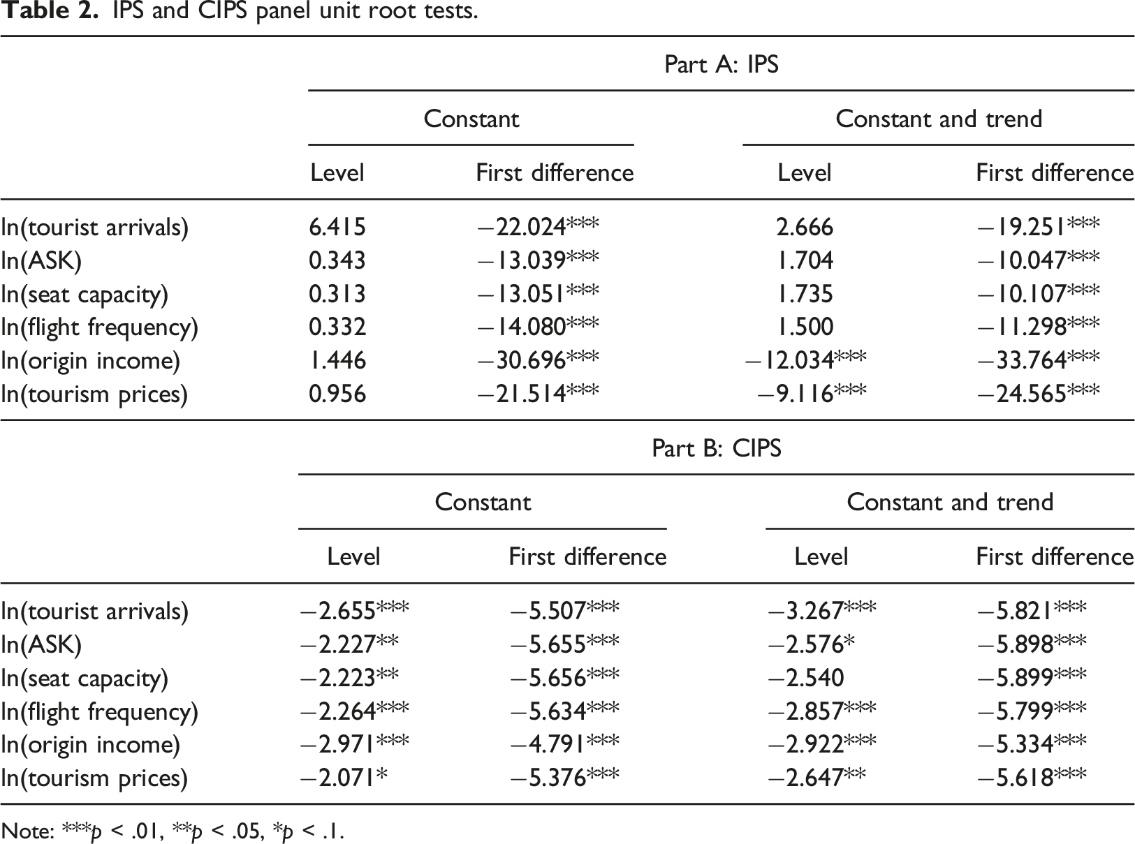
Note: ***p < .01, **p < .05, *p < .1.

Panel cointegration tests

Before estimating the CS-ARDL model, two types of panel cointegration tests are implemented to verify whether a cointegrating relationship exists between the studied variables, namely the Pedroni (1999) test and the Westerlund (2008) test. The residual-based Pedroni (1999) test verifies the stationarity of the OLS residuals for the studied variables. The null hypothesis of no cointegration is against the alternative hypothesis that the studied variables are cointegrated in all sections. However, this residual-based panel cointegration test suffers from loss of power if the imposed common factor restriction1 is not satisfied (Westerlund, 2008). In contrast, the error correction model-based Westerlund (2008) test removes the common factor restriction and allows for different long-term and short-term adjustment processes. Essentially, the Westerlund (2008) test rejects the null hypothesis of no cointegration in case the error correction coefficient is significantly different from zero2. It provides two types of test statistics, namely the group mean statistics ( $G_{α}$ and $G_{τ}$ ) and the panel statistics ( $P_{α}$ and $P_{τ}$ ). The panel statistics differ from the group mean statistics in that the former are based on pooling the information about the error correction across sections. As a result, the group mean statistics allow for heterogeneity of the error correction coefficients. The null hypothesis of no cointegration is against the alternative hypothesis that there is cointegration for at least one section. In contrast, the panel statistics assume homogeneity of the error correction coefficients. The null hypothesis of no cointegration is against the alternative hypothesis that the panel as a whole is cointegrated. On the other hand, compared to $G_{α}$ and $P_{α}$ , $G_{τ}$ and $P_{τ}$ are normalized by the number of time periods and thus, have higher power according to the Monte Carlo simulation (Westerlund, 2008). In addition to the ordinary p-values, we generate the robust p-values by the bootstrap approach of 100 times, providing cross-sectionally dependent-robust results.

Table 3 reports the results of the panel cointegration tests. Based on the Pedroni (1999) test, there is overwhelming evidence to support the cointegrating relationship between the studied variables in all cases (model specifications with all three measures of air transport capacity). Based on the Westerlund (2008) test, the ordinary p-values for all four tests provide strong evidence of the cointegrating relationship between the studied variables. However, the robust p-values for

G_{α}

and

P_{α}

are larger than 0.1 in the model specifications with ASK and seat capacity. As both the ordinary and robust p-values for the higher power statistics,

G_{τ}

and

P_{τ}

, demonstrate significant statistics, we conclude that a cointegrating relationship still exists in these cases.

Table 3.

Pedroni (1999) and Westerlund (2008) panel cointegration tests.

Part A: Pedroni (1999) test
	With ln(ASK)			With ln(seat capacity)			With ln(flight frequency)
ln(tourists)	ADF t-statistic		p-value	ADF t-statistic		p-value	ADF t-statistic	p-value
ln(tourists)	−44.918		0.00	−45.072		0.00	−46.432	0.00
	Part B: Westerlund (2008) test
	With ASK			With seat capacity			With flight frequency
	Value	p-val.	Robust p-val.	Value	p-val.	Robust p-val.	Value	p-val.	Robust p-val.
$G_{t}$	−4.758	.00	0.00	−4.741	.00	0.00	−4.968	.00	0.00
$G_{a}$	−20.689	.00	0.13	−20.537	.00	0.13	−21.311	.00	0.04
$P_{t}$	−37.686	.00	0.00	−37.863	.00	0.00	−38.750	.00	0.00
$P_{a}$	−23.389	.00	0.18	−23.398	.00	0.19	−24.627	.00	0.04

Granger causality tests

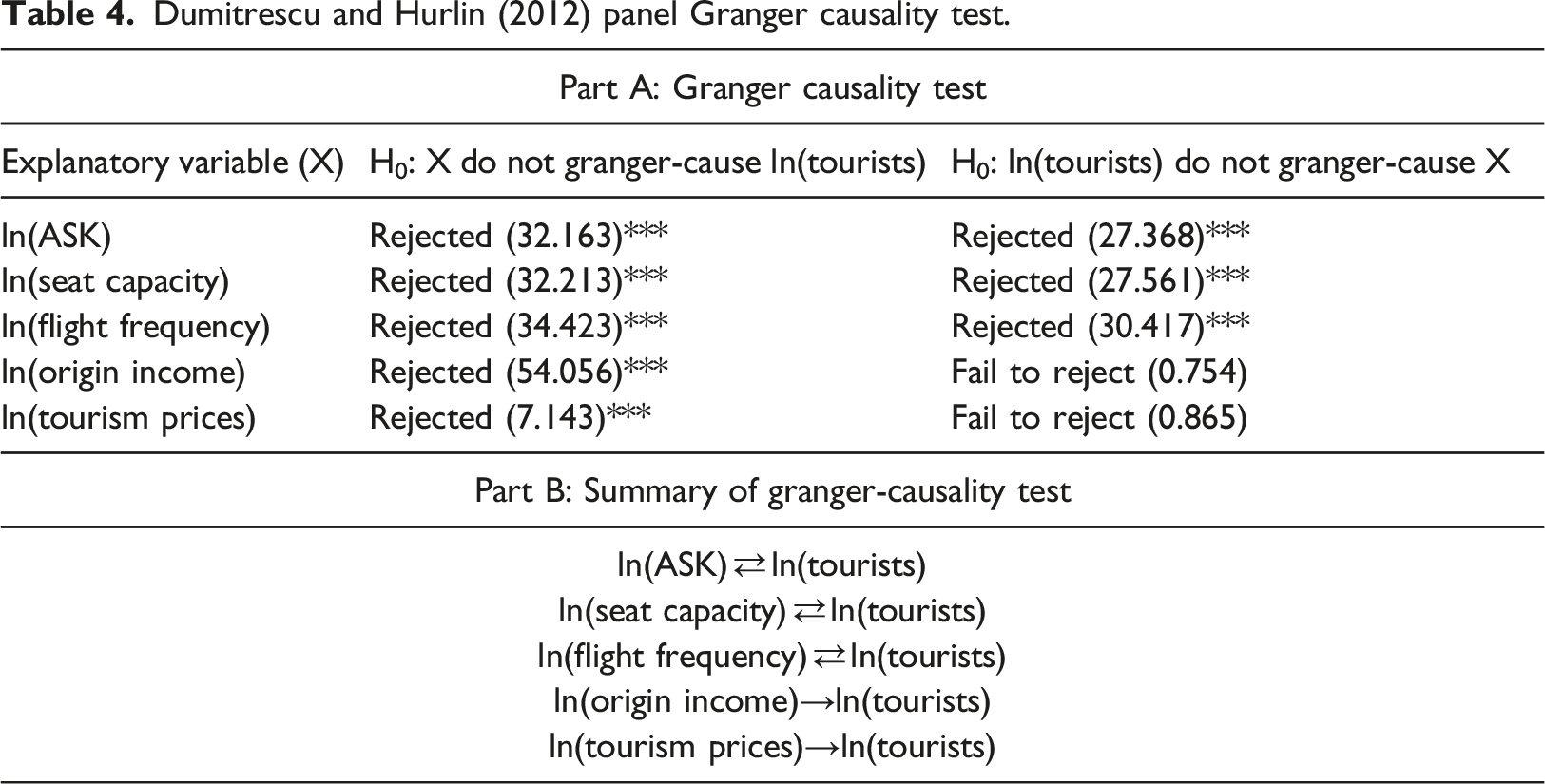
The existence of cointegration indicates causality, at least in one direction (Tano, 1993). To determine the direction(s) of the causality between the studied variables, we employ the Dumitrescu and Hurlin (2012) test of Granger causality for panel data. The Dumitrescu and Hurlin (2012) test is an extension of the Granger (1969) causality test for time series. In essence, the Granger (1969) causality test relies on the idea that if past information about $x$ is a significant predictor of the contemporary $y$ even when past information about $y$ has been included in the model, then $x$ is believed to have causal effect on $y$ .

Table 4 reports the empirical results of the Dumitrescu and Hurlin (2012) test of Granger causality between tourist arrivals, air transport capacity (ASK, seat capacity, and flight frequency), origin income, and tourism prices in both directions. As shown, there exists bidirectional causality between tourist arrivals and all three measures of air transport capacity, whereas only unidirectional causality is observed for origin income and tourism prices. These observations provide strong evidence to support the commonly recognized endogenous relationship between air transport capacity and tourism demand, while origin income and tourism prices can be considered exogenous in our empirical model.

Table 4.

Dumitrescu and Hurlin (2012) panel Granger causality test.

Part A: Granger causality test
Explanatory variable (X)	H₀: X do not granger-cause ln(tourists)	H₀: ln(tourists) do not granger-cause X
ln(ASK)	Rejected (32.163)***	Rejected (27.368)***
ln(seat capacity)	Rejected (32.213)***	Rejected (27.561)***
ln(flight frequency)	Rejected (34.423)***	Rejected (30.417)***
ln(origin income)	Rejected (54.056)***	Fail to reject (0.754)
ln(tourism prices)	Rejected (7.143)***	Fail to reject (0.865)
Part B: Summary of granger-causality test
ln(ASK)⇄ln(tourists)
ln(seat capacity)⇄ln(tourists)
ln(flight frequency)⇄ln(tourists)
ln(origin income)→ln(tourists)
ln(tourism prices)→ln(tourists)

Full sample analyses

To begin with, we estimate the auxiliary regressions to obtain the predicted values of the air transport capacity variable using the instrument (HHI), alongside the two exogenous variables (origin income and tourism prices), as well as the seasonal dummy variables. Fixed effects are incorporated in the auxiliary regressions. As reported in Table 5, HHI is shown to have significant negative effect on all three measures of air transport capacity (−0.784∼−0.710). This suggests that 10% increase in airline market competition in terms of HHI leads to 7.10%–7.84% increase in air transport capacity. This result is in line with the study by Mohammadian et al. (2019), which finds in the context of domestic market of Australia, that 10% increase in airline market competition measured by HHI results in 7%, 31%, and 8% increases in flight frequency on the short-, medium-, and long-haul routes, respectively.

Table 5.

Auxiliary regressions for the CS-ARDL model specifications with instrument.

	(1)	(2)	(3)
	ln(ASK)	ln(seat capacity)	ln(flight frequency)
ln(HHI)	−0.710*** (−9.578)	−0.720*** (−9.665)	−0.784*** (−10.71)
ln(origin income)	0.770*** (5.173)	0.766*** (5.167)	0.769*** (5.053)
ln(tourism prices)	0.170 (1.429)	0.172 (1.487)	0.0827 (0.737)
Q1	−0.0162** (−2.443)	−0.0162** (−2.445)	−0.0154** (−2.448)
Q2	−0.0694*** (−7.082)	−0.0693*** (−7.060)	−0.0602*** (−6.620)
Q3	−0.0341*** (−3.239)	−0.0339*** (−3.235)	−0.0263*** (−2.765)
Constant	9.882*** (5.535)	1.307 (0.736)	−4.133** (−2.239)
Observations	2304	2304	2304
No. of O-D pairs	48	48	48
R-squared	0.488	0.493	0.539

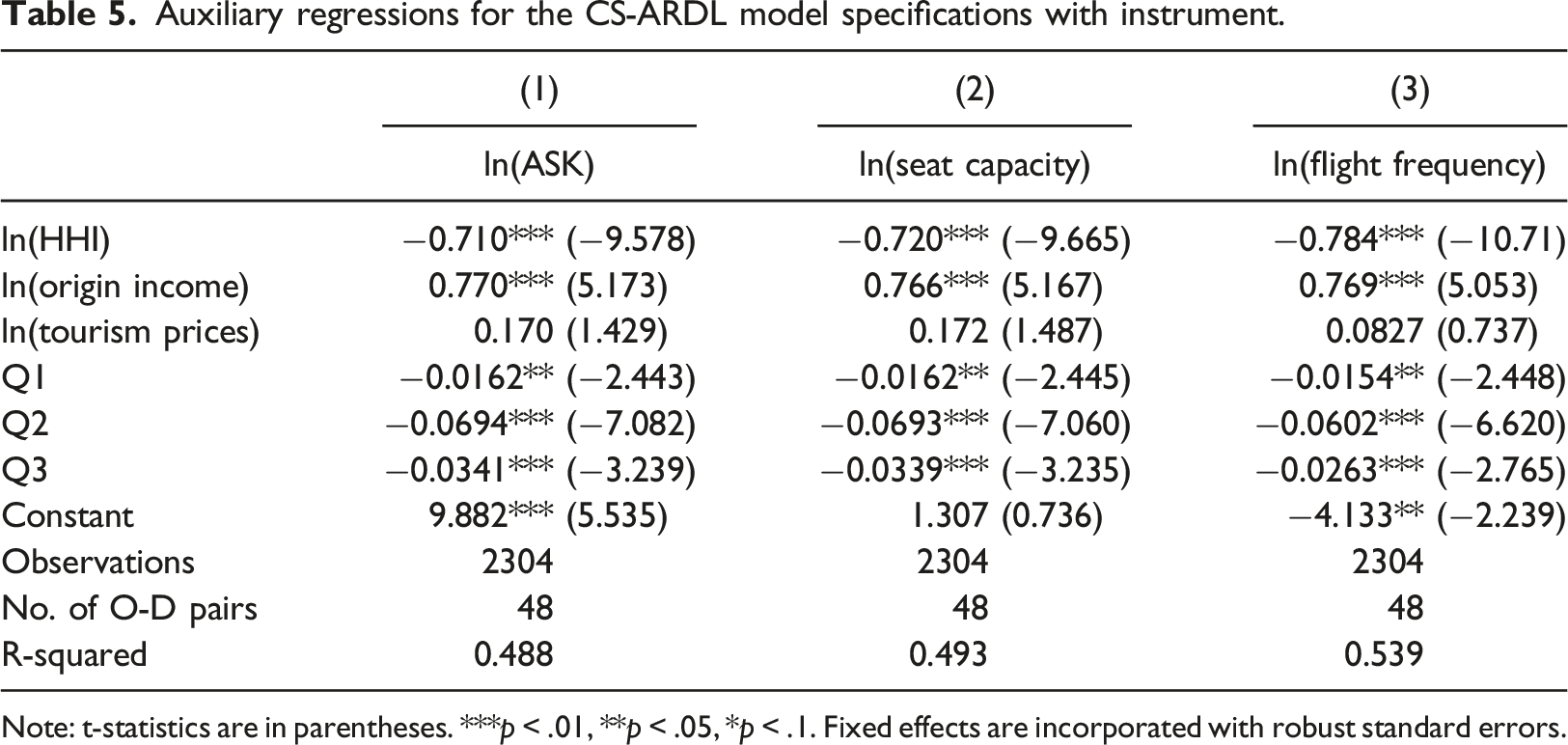
Note: t-statistics are in parentheses. ***p < .01, **p < .05, *p < .1. Fixed effects are incorporated with robust standard errors.

Tables 6-8 report the empirical results using the (i) conventional ARDL, (ii) CS-ARDL, and (iii) CS-ARDL with instrument based on the MG and PMG estimators. For the (ii) CS-ARDL and (iii) CS-ARDL with instrument, the current and lagged values of the cross-sectional averages of the dependent and explanatory variables are incorporated to mitigate the cross-sectional dependence in residuals. The cross-sectional averages of the studied variables have accounted for the deterministic effects (i.e., intercept, seasonality, time trend, one-off event dummy). Hence, unlike the conventional ARDL model, we do not incorporate the intercept and seasonal dummy variables in the CS-ARDL model specifications (Fuleky et al., 2014). In particular, for the (iii) CS-ARDL with instrument, the predicted values of the air transport capacity generated from the auxiliary regressions are incorporated in the regression model³.

Table 6.

Empirical results for the model specifications with ASK.

	(4)	(5)	(6)	(7)	(8)	(9)
	Conventional ARDL		CS-ARDL		CS-ARDL with instrument
	MG	PMG	MG	PMG	MG	PMG
Long-term coefficients
ln(ASK)	0.257*** (5.883)	0.320*** (24.74)	0.308*** (4.221)	0.297*** (11.28)	0.416** (2.406)	0.475*** (10.69)
ln(origin income)	1.424*** (9.989)	1.152*** (41.23)	0.161 (0.424)	0.511*** (4.786)	−0.331 (−0.664)	0.489*** (4.572)
ln(tourism prices)	−0.396*** (−4.384)	−0.629*** (−26.05)	−0.198* (−1.745)	−0.0902** (−2.440)	−0.298** (−2.495)	−0.179*** (-4.794)
Error correction	−0.768*** (−18.54)	−0.457*** (−30.74)	−1.009*** (−22.49)	−0.894*** (−29.03)	−1.022*** (−23.68)	−0.849*** (−29.26)
Observations	2256	2256	2256	2256	2256	2256
R-squared	0.106	0.159	0.323	0.497	0.351	0.524
No. Of O-D pairs	48	48	48	48	48	48
CD test	13.21	12.27	−1.405	−1.932	−1.420	−1.891
p-value of CD test	0	0	0.160	0.0533	0.156	0.0586
Hausman test	104.62		6.25		2.89
p-value of Hausman test	0		0.1816		0.5772

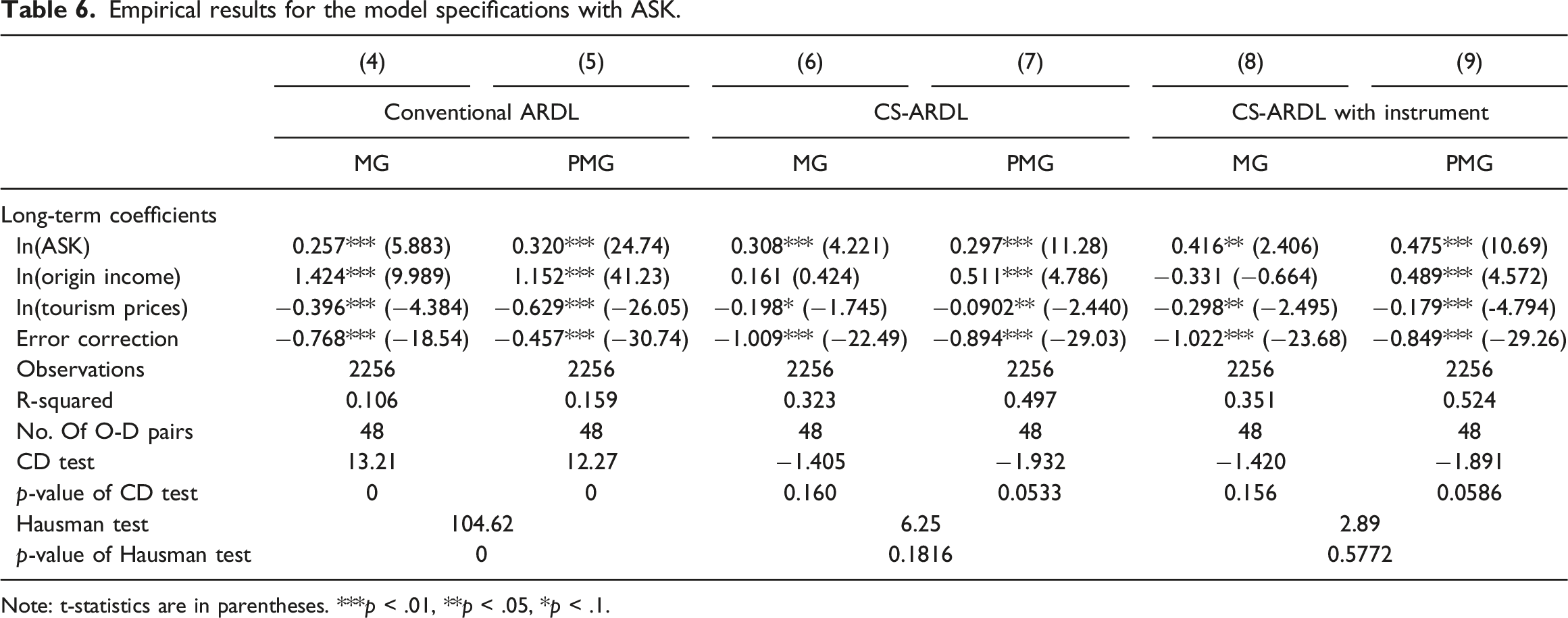
Note: t-statistics are in parentheses. ***p < .01, **p < .05, *p < .1.

Table 7.

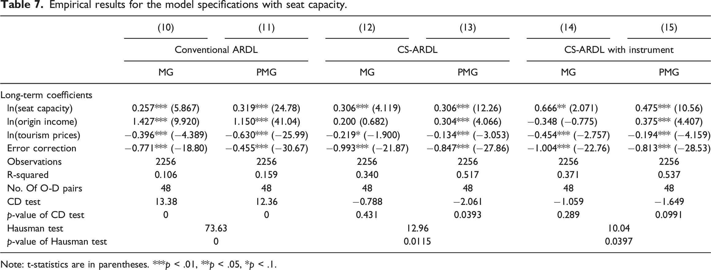
Empirical results for the model specifications with seat capacity.

	(10)	(11)	(12)	(13)	(14)	(15)
	Conventional ARDL		CS-ARDL		CS-ARDL with instrument
	MG	PMG	MG	PMG	MG	PMG
Long-term coefficients
ln(seat capacity)	0.257*** (5.867)	0.319*** (24.78)	0.306*** (4.119)	0.306*** (12.26)	0.666** (2.071)	0.475*** (10.56)
ln(origin income)	1.427*** (9.920)	1.150*** (41.04)	0.200 (0.682)	0.304*** (4.066)	−0.348 (−0.775)	0.375*** (4.407)
ln(tourism prices)	−0.396*** (−4.389)	−0.630*** (−25.99)	−0.219* (−1.900)	−0.134*** (−3.053)	−0.454*** (−2.757)	−0.194*** (−4.159)
Error correction	−0.771*** (−18.80)	−0.455*** (−30.67)	−0.993*** (−21.87)	−0.847*** (−27.86)	−1.004*** (−22.76)	−0.813*** (−28.53)
Observations	2256	2256	2256	2256	2256	2256
R-squared	0.106	0.159	0.340	0.517	0.371	0.537
No. Of O-D pairs	48	48	48	48	48	48
CD test	13.38	12.36	−0.788	−2.061	−1.059	−1.649
p-value of CD test	0	0	0.431	0.0393	0.289	0.0991
Hausman test	73.63		12.96		10.04
p-value of Hausman test	0		0.0115		0.0397

Note: t-statistics are in parentheses. ***p < .01, **p < .05, *p < .1.

Table 8.

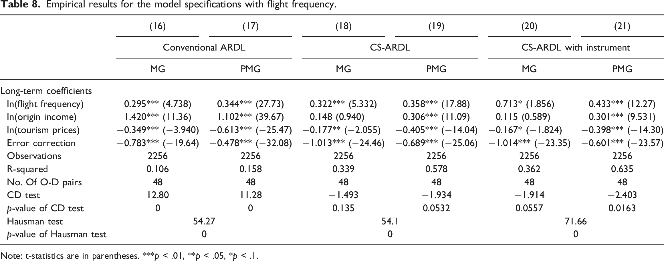
Empirical results for the model specifications with flight frequency.

	(16)	(17)	(18)	(19)	(20)	(21)
	Conventional ARDL		CS-ARDL		CS-ARDL with instrument
	MG	PMG	MG	PMG	MG	PMG
Long-term coefficients
ln(flight frequency)	0.295*** (4.738)	0.344*** (27.73)	0.322*** (5.332)	0.358*** (17.88)	0.713* (1.856)	0.433*** (12.27)
ln(origin income)	1.420*** (11.36)	1.102*** (39.67)	0.148 (0.940)	0.306*** (11.09)	0.115 (0.589)	0.301*** (9.531)
ln(tourism prices)	−0.349*** (−3.940)	−0.613*** (−25.47)	−0.177** (−2.055)	−0.405*** (−14.04)	−0.167* (−1.824)	−0.398*** (−14.30)
Error correction	−0.783*** (−19.64)	−0.478*** (−32.08)	−1.013*** (−24.46)	−0.689*** (−25.06)	−1.014*** (−23.35)	−0.601*** (−23.57)
Observations	2256	2256	2256	2256	2256	2256
R-squared	0.106	0.158	0.339	0.578	0.362	0.635
No. Of O-D pairs	48	48	48	48	48	48
CD test	12.80	11.28	−1.493	−1.934	−1.914	−2.403
p-value of CD test	0	0	0.135	0.0532	0.0557	0.0163
Hausman test	54.27		54.1		71.66
p-value of Hausman test	0		0		0

Note: t-statistics are in parentheses. ***p < .01, **p < .05, *p < .1.

Table 6 demonstrates the long-term coefficient estimates of ASK on tourism demand. ASK is given by the number of available seats multiplied by the total travel distance in kilometer. Thus, a seat on a long-haul flight produces greater ASK than a seat on a short-haul flight. Across Columns (4)–(9), we observe that ASK has significant positive effect on tourism demand. Under the conventional ARDL model specifications, the long-term coefficient estimates of ASK are 0.257 and 0.320 using the MG and PMG estimators, respectively, whereas these two numbers are 0.308 and 0.297 under the CS-ARDL model specifications. However, the conventional ARDL model specifications suffer from cross-sectional dependence since the Pesaran (2021) CD test statistics show overwhelming evidence of rejecting the null hypothesis of no cross-sectional dependence in all cases. In contrast, under the CS-ARDL model specifications, cross-sectional dependence is effectively mitigated, as indicated by the corresponding CD test statistics. The F-statistics of the Hausman (1978) test suggest that, under the CS-ARDL model specifications, the MG and PMG estimators generate systematically similar estimates and there is long-term slope homogeneity across the O-D pairs. Thus, the PMG estimates are consistent and more efficient. Notably, after mitigating the endogeneity problem using the instrument, we obtain a slightly larger effect of ASK (0.416–0.475), as shown in Columns (8)–(9). This suggests that, without considering the endogeneity problem, a downward bias may exist on the coefficient estimate of air transport capacity. Biased estimations are also observed in some passenger demand studies focusing on the effect of airfare if the endogeneity problem is not considered (e.g., Lurkin et al., 2017; Morlotti et al., 2017; Mumbower et al., 2014; Perera and Tan, 2019).

Regarding the long-term effect of origin income, we observe that the corresponding long-term coefficient estimates are larger than 1 under the conventional ARDL model specifications. In other words, 1% increase in origin income leads to more than 1% increase in tourist arrivals to Australia, implying that traveling to Australia is income elastic. This contrasts sharply with the results generated under the CS-ARDL model specifications, which indicate that tourism demand is insensitive to changes in origin income in the long term (0.489–0.511, as indicated in Columns (7) and (9)). Additionally, the long-term coefficient estimates of tourism prices under the conventional ARDL model specifications (−0.692∼−0.396) are larger in size than under the CS-ARDL model specifications (−0.298∼−0.0902). We postulate that the conventional ARDL model overestimates the effect of income and tourism prices due to the cross-sectional dependence problem. Under the CS-ARDL model specifications, the estimated long-term income and tourism price elasticities concerning the international tourism demand of Australia are similar to the ones found by Seetaram (2010) and Ghosh (2022), who also adopt the dynamic panel cointegration approach to examine the inbound tourism demand of Australia during 1991–2007 and 2007–2020, respectively. In contrast, the papers published between 1961 and 2011 in the meta-analysis by Peng et al. (2015) show that international tourists to Oceania (where Australia is the dominant destination) exhibit income elasticity value of 2.067 and tourism price elasticity −0.844. As can be seen, the estimates of income and tourism price elasticities for inbound tourism demand of Australia tend to be smaller in size in more recent studies.

Furthermore, the estimated error correction coefficients are significant negative. This strongly suggests that tourist arrivals, air transport capacity, origin income, and tourism prices are cointegrated, which align with the results of the panel cointegration tests reported in Table 3. The error correction coefficient (aka the speed of adjustment) measures how fast the dependent variable returns from its short-term deviation to the long-term equilibrium with the other variables. The value of −1 indicates that tourist arrivals return to the long-term equilibrium by one period, equivalent to a quarter in our study. This is the situation when the empirical model is estimated by MG under the CS-ARDL model specifications (as shown in Columns (6) and (8)). In contrast, when the empirical model is estimated by PMG under the CS-ARDL model specifications, the estimated error correction coefficients range between −0.894 and −0.849, suggesting that it takes more than a quarter for tourist arrivals to return to the long-term equilibrium.

For comparative purposes and as a robustness check, we also utilize seat capacity and flight frequency as alternative measures of air transport capacity (as shown in Table 7 and Table 8).

Unlike ASK, seat capacity does not account for flight distance, whereas flight frequency does not account for aircraft size and flight distance. Generally speaking, the estimated long-term coefficients of air transport capacity, origin income, and tourism prices reported in Table 7 and Table 8 are similar to Table 6 in terms of the parameter estimates’ significance level, sign, and size. This provides further support that the ARDL model specifications used in our study can generate robust coefficient estimates depicting the cointegrating relationship between the variables of interest.

Subsample analyses (tourist arrivals by trip purpose)

Table 9 reports the empirical results for tourism demand for the three main trip purposes: business, holiday, and VFR, using the CS-ARDL with instrument. By analyzing tourist arrivals by trip purpose, we can compare how business and leisure (which includes holiday and VFR) tourists respond differently to air transport capacity, origin income, and tourism prices. As in the full sample analyses, we have noticed that the Hausman (1978) test supports utilizing the PMG estimator in the majority of the cases, we assume the long-term coefficients of the studied variables are homogenous across the O-D pairs. Therefore, we utilize the PMG estimator to generate estimates for the analyses of by-trip purpose tourists.

Table 9.

Empirical results for the CS-ARDL with instrument model specifications (by-trip purpose tourist arrivals).

	Business			Holiday			VFR
	(22)	(23)	(24)	(25)	(26)	(27)	(28)	(29)	(30)
	ASK	Seat	Frequency	ASK	Seat	Frequency	ASK	Seat	Frequency
Long-term coefficients
ln(capacity)	0.191** (2.214)	0.198** (2.363)	0.184** (2.345)	0.574*** (7.672)	0.567*** (7.525)	0.513*** (8.489)	0.393*** (7.707)	0.381*** (7.474)	0.353*** (7.793)
ln(origin income)	0.487 (1.301)	0.343 (0.976)	0.368 (0.864)	1.031*** (3.847)	0.758*** (3.363)	0.266*** (4.261)	0.360*** (2.647)	0.334*** (3.122)	0.173*** (6.139)
ln(tourism prices)	0.00341 (0.0207)	0.0282 (0.172)	0.0215 (0.125)	−0.163*** (−2.616)	−0.146** (−2.212)	−0.252*** (−5.206)	−0.152*** (−3.314)	−0.142*** (−2.822)	−0.291*** (−8.720)
Error correction	−0.992*** (−33.03)	−0.991*** (−32.81)	−0.992*** (−32.75)	−0.737*** (−19.10)	−0.739*** (−19.20)	−0.694*** (−19.88)	−0.868*** (−14.52)	−0.862*** (−14.46)	−0.779*** (−12.99)
Observations	2160	2160	2160	1920	1920	1920	2256	2256	2256
R-squared	0.441	0.439	0.438	0.511	0.512	0.546	0.545	0.548	0.585
Number of groups	48	48	48	48	48	48	48	48	48
CD test	−1.521	−1.814	−1.745	−0.810	−1.223	−1.551	0.00792	−0.278	0.461
p-value of CD test	0.128	0.0697	0.0809	0.418	0.221	0.121	0.994	0.781	0.644

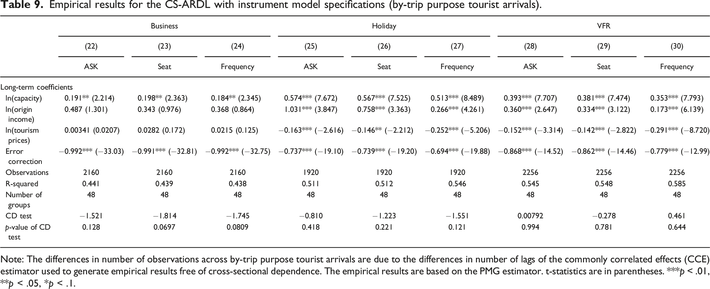
Note: The differences in number of observations across by-trip purpose tourist arrivals are due to the differences in number of lags of the commonly correlated effects (CCE) estimator used to generate empirical results free of cross-sectional dependence. The empirical results are based on the PMG estimator. t-statistics are in parentheses. ***p < .01, **p < .05, *p < .1.

As shown in Table 9, three observations can be highlighted. First, the estimated long-term coefficients of air transport capacity are significant at least at the 5% significance level for all the three measures and for all trip purposes. Specifically, the corresponding coefficient estimates for holiday tourists range between 0.513 and 0.574, the largest amongst all the trip purposes. While VFR tourists are also significantly influenced by air transport capacity to the destination, the size of the effect is smaller than that of holiday tourists, ranging between 0.353 and 0.393. This might be attributed to the fact that destination choices for VFR tourism are influenced by where their friends/relatives reside overseas; thus, increase in air transport capacity to Australia may have small influence on some VFR tourists if their friends/relatives do not live at that destination. Concerning business tourists, the long-term coefficient estimates of air transport capacity are the smallest among the three trip purposes. This makes sense if one accepts that business tourists will not necessarily travel to a destination because it is easy to get to, or simply because air transport is cheaper or available. And they are usually determined by the firm or the need to attend business activities. Unlike holiday or VFR travels which are usually planned several months in advance, business travel decisions may be made within a short time period before the departure date. As a result, the long-term effect of air transport on business tourism demand is also smaller than leisure tourism demand.

Second, as shown in Column (25), the significant long-term coefficient estimates of origin income for holiday tourists is 1.031, implying that holiday travel to Australia is income elastic. In contrast, we do not find a significant positive long-term effect of origin income on business tourists. This observation is consistent with the meta-analysis by Peng et al. (2015), which finds that holiday tourists are usually more influenced by origin income than business tourists. Third, we do not observe any significant effect of tourism prices on business tourists. The unresponsiveness to tourism prices by business tourists might be attributed to the possible situation that the employers fully or partially cover tourism expenditure for business travel. As such, demand for business travel might not be deterred by high tourism prices in the destination.

Discussion and implications

For a geographically remote destination such as Australia, the air transport and tourism industries are usually interdependent and require commonly coordinated and planned integration in the long term (Ivanova, 2017); thus, the long-term cointegrating relationship between them is of interest for facilitating aviation policymaking and understanding whether economic agents of travel sectors optimize behaviors with one another. The finding that there is a non-negligible generative effect of air capacity on demand has implications for competition policy and international air services agreements.

First, policymakers and regulators (e.g., Dept. Transport, the Australian Competition and Consumer Commission or ACCC) should aim to maintain competition in the Australian airline industry through a highly liberalized market, which can ensure a high level of international air transport capacity. It is important to note that there exists an innate misalignment in interest between the tourism destination and airlines. While the former focuses on economic benefits brought by tourist arrivals, the latter pays particular attention to revenue generated from passengers (not necessarily tourist arrivals) and operating costs. Therefore, airlines may restrict capacity and adopt price discrimination (aka yield management) to create as much revenue as possible with maximized load factor (Bergantino and Capozza, 2015; Hsu and Wen, 2003). However, destination policymakers can indirectly influence air transport capacity via the implementation of a relatively open international aviation policy through liberal bilateral air services agreements (Duval, 2008).

Second, air route development activities may involve direct or indirect subsidies to further boost direct air transport capacity for the purpose of developing longer-term tourism. According to Morrison and de Wit (2019), government subsidies have the same effect of lower operating costs, which, in game theoretic terms assuming a Cournot model, lead to a Nash equilibrium with a higher capacity level. However, it is important to note the empirical results of this study are for long-term cointegrating relationship; therefore, air route development activities must ensure consistent service levels for at least several years to observe the effect found in this analysis.

Conclusion

This study is the first attempt to conduct a panel cointegration analysis on the air transport capacity – tourism demand nexus. Cointegration analysis avoids the problem of spurious regression and multicollinearity, which can impact the accuracy and reliability of the empirical results. A panel time series dataset based on large cross-sections and long time horizon enables us to adopt a parsimonious model specification to generate robust coefficient estimates of air transport capacity. We employ the CS-ARDL model, developed by Chudik and Pesaran (2015), to examine the cointegrating relationship between tourist arrivals, air transport capacity, origin income, and tourism prices. We utilize the HHI as an instrument to mitigate the endogeneity problem arising from the commonly recognized bidirectional causality between air transport capacity and tourism demand.

Compared with other commonly used panel econometric techniques, the CS-ARDL model has a number of advantages in examining large-scale panel time series data. First, utilizing the MG/PMG estimator allows for slope heterogeneity across the O-D pairs. Second, by incorporating cross-sectional averages of the studied variables in the regression, the CS-ARDL model can effectively mitigate cross-sectional dependence in residuals. This is particularly important when examining data for tourist flows from a sample of origins to a common destination/country (Dogru et al., 2021). The results highlight that accounting for cross-sectional dependence changes income elasticity from elastic to inelastic. Thus, accounting for cross-sectional dependence when examining panel time series is necessary; otherwise, the practical implications generated from the empirical results might be misleading. Third, utilizing HHI as an instrument under the CS-ARDL model enables us to mitigate the endogeneity problem arising from the bidirectional causality between air transport capacity and tourism demand. As discussed earlier, coefficients of air transport capacity tend to be underestimated when the endogeneity problem is not adequately corrected for.

In general, the empirical results from the auxiliary regressions show that 10% increase in airline market competition measured by HHI leads to around 7% increase in air transport capacity. Then, using the predicted values of the air transport capacity obtained from the auxiliary regressions, we estimate the cointegrating relationship between tourism demand, air transport capacity, origin income, and tourism prices. Our study empirically demonstrates that 1% increase in ASK, seat capacity, or flight frequency results in 0.416%–0.713% increase in tourist arrivals to Australia in the long term. This estimate is more robust to potential biases that may be present in earlier studies. Furthermore, through analyses of tourist arrivals by trip purpose, we find that air transport capacity has greater influences on holiday and VFR tourists than business tourists.

This study can be extended in several ways in the future. First, restricted by the data for tourist arrivals, the cross-sections in our panel time series data refer to the pairs of origin country/market-Australian state, rather than the individual routes serviced by nonstop flights. The aggregation of individual routes assumes the utility functions of tourists are identical across all the routes for a specific O-D pair. Based on Morley et al. (2014), in examining data for tourism demand, high level of segmentation is preferred because it allows for heterogeneity of utility functions across a sample of routes investigated. Second, only pre-COVID observations are included in our panel time series data. Our cointegration analysis of air transport capacity and tourism demand is based on a long period of historical data. The econometric techniques may not capture the large structural change due to the recent unanticipated COVID shocks (Zhang et al., 2021). Future research may reexamine the air transport capacity–tourism demand relations for a sample of routes and integrate the Delphi adjustment method in conjunction with the CS-ARDL model to account for the COVID factor. The current study results, however, are still useful in highlighting the likely relations in the international travel sector under reasonably well-performing market conditions, which is often the type of environment promoted by many governments and destination marketing organizations (certainly in Australia) in regard to international aviation.

Footnotes

Acknowledgements

The authors are grateful to the editor and two anonymous reviewers for helpful comments and suggestions. The authors would like to acknowledge the aviation data provided by Cirium - RELX group. The 1st and 3rd authors wish to acknowledge the funding support of the University of Macau Research Grants (File no. SP2022-00005-DRTM and MYRG2020-00235-FBA).

Declaration of conflicting interests

The author(s) declared no potential conflicts of interest with respect to the research, authorship, and/or publication of this article.

Funding

The author(s) disclosed receipt of the following financial support for the research, authorship, and/or publication of this article: This work was supported by the University of Macau (MYRG2020-00235-FBA and SP2022-00005-DRTM).

Orcid iDs

Rockie U Kei Kuok

Tay T.R. Koo

Notes

Author biographies

Rockie U Kei Kuok obtained his PhD from the Faculty of Business Administration, University of Macau. He is a full-time A320 airline pilot based in Macau and a sessional academic with the School of Aviation, UNSW Sydney, as well as Chartered Financial Analyst (CFA) Level 3 Candidate. His research interests are in aviation and tourism economics/econometrics.

Tay T.R. Koo is Senior Lecturer in the School of Aviation at UNSW Sydney. His academic background is in geography and economics with emphasis on sustainable aviation and travel management. His research interest involves the study of aviation consumers, air route development and research methodologies in spatial impacts of tourism.

Christine Lim is Associate Professor and researcher in tourism demand modeling at the Faculty of Business Administration, University of Macau.

References

Alderighi

Gaggero

(2019) Flight availability and international tourism flows. Annals of Tourism Research 79: 102642.

Alsumairi

Hong Tsui

(2017) A case study: the impact of low-cost carriers on inbound tourism of Saudi Arabia. Journal of Air Transport Management 62: 129–145.

Australian Bureau of Statistics (2020) Overall Arrivals and Departure. Available at: https://data.gov.au/(accessed 16 June 2022).

Balli

Tsui

WHK

(2019) International tourism demand, number of airline seats and trade triangle: evidence from New Zealand partners. Tourism Economics 25(1): 132–144.

Bergantino

Capozza

(2015) One price for all? price discrimination and market captivity: evidence from the Italian city-pair markets. Transportation Research Part A: Policy and Practice 75: 231–244.

Cattaneo

Malighetti

Redondi

, et al. (2018) Changes in frequencies and price variations on point-to-point routes: the case of easyJet. Transportation Research Part A: Policy and Practice 112: 60–70.

Christoffersen

Diebold

(1997) Optimal prediction under asymmetric loss. Econometric Theory 13: 808–817.

Chudik

Pesaran

(2015) Common correlated effects estimation of heterogeneous dynamic panel data models with weakly exogenous regressors. Journal of Econometrics 188(2): 393–420.

Chung

Whang

(2011) The impact of low cost carriers on Korean Island tourism. Journal of Transport Geography 19(6): 1335–1340.

10.

Cirium (2020) Aviation analytics database. Available at: https://www.cirium.com/(accessed 16 August 2021).

11.

Clements

Hendry

(1995) Forecasting in cointegrated systems. Journal of Applied Econometrics 10: 127–146.

12.

Crouch

(1995) A meta-analysis of tourism demand. Annals of Tourism Research 22(1): 103–118.

13.

Demir

Gozgor

Paramati

(2020) To what extend economic uncertainty effects tourism investments? evidence from OECD and non-OECD economies. Tourism Management Perspectives 36: 100758.

14.

Dogru

Bulut

Sirakaya-Turk

(2021) Modeling tourism demand: theoretical and empirical considerations for future research. Tourism Economics 27(4): 874–889.

15.

Douglas

Miller

(1974) Quality competition, industry equilibrium, and efficiency in the price-constrained airline market. The American Economic Review 64(4): 657–669.

16.

Dumitrescu

E-I

Hurlin

(2012) Testing for granger non-causality in heterogeneous panels. Economic Modelling 29: 1450–1460.

17.

Duval

(2008) Regulation, competition and the politics of air access across the Pacific. Journal of Air Transport Management 14: 237–242.

18.

Duval

Schiff

(2011) Effect of air services availability on international visitors to New Zealand. Journal of Air Transport Management 17(3): 175–180.

19.

Engle

Granger

CWJ

(1987) Co-integration and error correction: representation, estimation, and testing. Econometrica 55: 251–276.

20.

Frees

(1995) Assessing cross-sectional correlation in panel data. Journal of Econometrics 69(2): 393–414.

21.

Fuleky

Zhao

Bonham

(2014) Estimating demand elasticities in non-stationary panels: the case of Hawaii tourism. Annals of Tourism Research 44: 131–142.

22.

Gallet

Doucouliagos

(2014) The income elasticity of air travel: a meta-analysis. Annals of Tourism Research 49: 141–155.

23.

Ghosh

(2022) Modelling inbound international tourism demand in Australia: lessons from the pandemics. International Journal of Tourism Research 24(1): 71–81.

24.

Granger

CWJ

(1969) Investigating causal relations by econometric models and cross-spectral methods. Econometrica 37: 424–438.

25.

Granger

CWJ

(2009) Developments in the study of cointegrated economic variables. Oxford Bulletin of Economics and Statistics 48(3): 213–228.

26.

Granger

CWJ

(2004) Time series analysis, cointegration, and applications. American Economic Review 94: 421–425.

27.

Greene

(2003) Econometric analysis. India: Pearson Education.

28.

Gunter

Önder

Smeral

(2019) Scientific value of econometric tourism demand studies. Annals of Tourism Research 78: 102738.

29.

Hausman

(1978) Specification tests in econometrics. Econometrica 46: 1251–1271.

30.

Herzer

(2019) The long-run effect of aid on health: evidence from panel cointegration analysis. Applied Economics 51(12): 1319–1338.

31.

Hsu

Wen

(2003) Determining flight frequencies on an airline network with demand-supply interactions. Transportation Research Part E: Logistics and Transportation Review 39: 417–441.

32.

Pesaran

Shin

(2003) Testing for unit roots in heterogeneous panels. Journal of Econometrics 115(1): 53–74.

33.

Ivanova

(2017) Air Transport–Tourism Nexus: A Destination Management Perspective. Varna: Zangador.

34.

Kao

(1999) Spurious regression and residual-based tests for cointegration in panel data. Journal of Econometrics 90(1): 1–44.

35.

Koo

TTR

Lim

Dobruszkes

(2017) Causality in direct air services and tourism demand. Annals of Tourism Research 67: 67–77.

36.

Koo

TTR

Tan

Duval

(2018) The effect of levels of air service availability on inbound tourism demand from Asia to Australia. In: Airline Economics in Asia. Bingley, UK: Emerald Publishing Limited, pp. 145–167

37.

Koo

TTR

Tan

Duval

(2013) Direct air transport and demand interaction: a vector error-correction model approach. Journal of Air Transport Management 28: 14–19.

38.

Kulendran

Witt

(2001) Cointegration versus least squares regression. Annals of Tourism Research 28(2): 291–311.

39.

Kuok

RUK

Koo

TTR

Lim

(2023) Economic policy uncertainty and international tourism demand: a global vector autoregressive approach. Journal of Travel Research 62(3): 540–562.

40.

Lee

Olasehinde‐Williams

Akadiri

(2021) Geopolitical risk and tourism: evidence from dynamic heterogeneous panel models. International Journal of Tourism Research 23(1): 26–38.

41.

WongYan

SongWei

, et al. (2006) Tourism demand forecasting: a time varying parameter error correction model. Journal of Travel Research 21: 175-178.

42.

Lim

(1997a) An econometric classification and review of international tourism demand models. Tourism Economics 3(1): 69–81.

43.

Lim

(1997b) Review of international tourism demand models. Annals of Tourism Research 24(4): 835–849.

44.

Lim

(1999) A meta-analytic review of international tourism demand. Journal of Travel Research 37(3): 273–284.

45.

Lurkin

Garrow

Higgins

, et al. (2017) Accounting for price endogeneity in airline itinerary choice models: an application to Continental US markets. Transportation Research Part A: Policy and Practice 100: 228–246.

46.

Lutkepohl

Kratzig

(2004) Applied Time Series Econometrics. Cambridge, England: Cambridge University Press.

47.

Mazzola

Cira

Ruggieri

, et al. (2022) Air transport and tourism flows to islands: a panel analysis for southern European countries. International Journal of Tourism Research 24: 639–652.

48.

Mohammadian

Abareshi

Abbasi

, et al. (2019) Airline capacity decisions under supply-demand equilibrium of Australia’s domestic aviation market. Transportation Research Part A: Policy and Practice 119: 108–121.

49.

Morley

Rossello

Santana-Gallego

(2014) Gravity models for tourism demand: theory and use. Annals of Tourism Research 48: 1–10.

50.

Morlotti

Cattaneo

Malighetti

, et al. (2017) Multi-dimensional price elasticity for leisure and business destinations in the low-cost air transport market: evidence from easyJet. Tourism Management 61: 23–34.

51.

Morrison

de Wit

(2019) US open skies agreements and unlevel playing fields. Journal of Air Transport Management 74: 30–38.

52.

Mumbower

Garrow

Higgins

(2014) Estimating flight-level price elasticities using online airline data: a first step toward integrating pricing, demand, and revenue optimization. Transportation Research Part A: Policy and Practice 66: 196–212.

53.

Pedroni

(1999) Critical values for cointegration tests in heterogeneous panels with multiple regressors. Oxford Bulletin of Economics and Statistics 61(S1): 653–670.

54.

Peng

Song

Crouch

(2014) A meta-analysis of international tourism demand forecasting and implications for practice. Tourism Management 45: 181–193.

55.

Peng

Song

Crouch

, et al. (2015) A meta-analysis of international tourism demand elasticities. Journal of Travel Research 54(5): 611–633.

56.

Perera

Tan

(2019) In search of the “Right Price” for air travel: first steps towards estimating granular price-demand elasticity. Transportation Research Part A: Policy and Practice 130: 557–569.

57.

Pesaran

Smith

(1995) Estimating long-run relationships from dynamic heterogeneous panels. Journal of Econometrics 68(1): 79–113.

58.

Pesaran

Shin

Smith

(2001) Bounds testing approaches to the analysis of level relationships. Journal of Applied Econometrics 16(3): 289–326.

59.

Pesaran

Shin

Smith

(1999) Pooled mean group estimation of dynamic heterogeneous panels. Journal of the American Statistical Association 94(446): 621–634.

60.

Pesaran

(2006) Estimation and inference in large heterogeneous panels with a multifactor error structure. Econometrica 74(4): 967–1012.

61.

Pesaran

(2007) A simple panel unit root test in the presence of cross‐section dependence. Journal of Applied Econometrics 22(2): 265–312.

62.

Pesaran

(2021) General diagnostic tests for cross-sectional dependence in panels. Empirical Economics 60: 13–50.

63.

Pitfield

Caves

Quddus

(2010) Airline strategies for aircraft size and airline frequency with changing demand and competition: a simultaneous-equations approach for traffic on the north Atlantic. Journal of Air Transport Management 16: 151–158.

64.

Rey

Myro

Galera

(2011) Effect of low-cost airlines on tourism in Spain. A dynamic panel data model. Journal of Air Transport Management 17(3): 163–167.

65.

Salesi

Tsui

WHK

, et al. (2021) The nexus of aviation and tourism growth in the South Pacific Region. Asia Pacific Journal of Tourism Research 26(5): 557–578.

66.

Seetaram

(2010) Use of dynamic panel cointegration approach to model international arrivals to Australia. Journal of Travel Research 49(4): 414–422.

67.

Shafiullah

Okafor

Khalid

(2019) Determinants of international tourism demand: evidence from Australian states and territories. Tourism Economics 25(2): 274–296.

68.

Spasojevic

Lohmann

(2022) Air route development-Lessons from Australia. Journal of Air Transport Management 104: 102274.

69.

Tano

(1993) The added worker effect: a causality test. Economics Letters 43: 111–117.

70.

Tsui

KWH

Tan

Chow

CKW

, et al. (2019) Regional airline capacity, tourism demand and housing prices: a case study of New Zealand. Transport Policy 77: 8–22.

71.

Hong Tsui

(2017) Does a low-cost carrier lead the domestic tourism demand and growth of New Zealand? Tourism Management 60: 390–403.

72.

Tveteras

Roll

(2014) Nonstop flights and tourist arrivals. Tourism Economics 20(1): 5–20.

73.

Westerlund

(2008) Panel cointegration tests of the Fisher effect. Journal of Applied Econometrics 23(2): 193–233.

74.

Zhang

Song

Wen

, et al. (2021) Forecasting tourism recovery amid COVID-19. Annals of Tourism Research 87: 103149.