Seismic fragility assessment of long-span cable-stayed bridges in China

Abstract

In the existing fragility assessment, most bridges are short-span bridges and a few bridges have long spans such as cable-stayed bridges. In this study, a procedure is proposed to conduct the component and system seismic fragility analysis of long-span cable-stayed bridges. Three critical issues are addressed in the procedure: (1) the optimal intensity measure of cable-stayed bridges, (2) limit state models of various components, and (3) contribution of individual components to the entire system failure of bridges. This study chooses a long-span cable-stayed bridge with the most common configuration in China and builds the numerical model of its multiple components using OpenSEES that can account for their nonlinear response and uncertainties in the ground motion and material properties. Four typical intensity measures are compared with respect to four characteristic properties including efficiency, practicality, sufficiency, and proficiency. Peak ground velocity turns out to be the optimal intensity measure. Limit states of pylon sections are derived by a numerical simulation based on pushover analysis and China’s guidelines. The pushover results indicate that the limit state of their section curvature depends highly on the section type and axial compression coefficient. A joint probabilistic seismic demand model and Monte Carlo simulation are employed to obtain an accurate system fragility estimate of cable-stayed bridges by accounting for the contribution of each component to the overall bridge system. The system fragility curves based on Monte Carlo simulation lie much closer to the upper bound fragilities given small correlation coefficients, implying that seismic demands of various components conditioned on the peak ground velocity are not correlated.

Keywords

cable-stayed bridges component and system fragility intensity measure Monte Carlo simulation probabilistic seismic demand model

Introduction

Seismic risk assessments play a crucial role in analyzing the potential losses and consequence of earthquakes. Outcomes of these assessments provide risk management, mitigation decision-making, and emergency planning and responses (Cornell et al., 2002; Mackie and Stojadinovic, 2001). The most common tool for this risk assessment is to develop fragility curves of structures (Basoz et al., 1999; Choi et al., 2004; Hwang et al., 2001; Nielson, 2005; Padgett and DesRoches, 2008; Pan et al., 2007; Ramanathan, 2012; Shinozuka et al., 2000a, 2000b). The fragility curves are conditional probability statements that give the likelihood that a structure will sustain or exceed a specified level of damage for a given ground motion intensity measure (IM).

In recent decades, cable-stayed bridges have been widely constructed around the world because of their aesthetics, efficient use of construction materials, and fast construction period (Pang et al., 2014; Ren and Obata, 1999). Nevertheless, most of the previous studies have focused on developing the fragility curve of short-span bridges. A few studies have assessed the seismic vulnerability of cable-stayed bridges. Pang et al. (2014) generated seismic fragility curves of a cable-stayed bridge based on the uniform design method. Barnawi and Dyke (2013) developed fragility curves of a benchmark cable-stayed bridge equipped with response modification systems. Casciati et al. (2008) evaluated the seismic vulnerability of a cable-stayed bridge with passive hysteretic devices in terms of damage exceedance probability. However, Barnawi and Dyke (2013), Casciati et al. (2008), and Pang et al. (2014) used the existing fragility modeling methodology developed for highway bridges with small span lengths without any modification for cable-stayed bridges. For example, these authors (1) adopted an optimal IM used in previous studies focusing on highway bridges for this class of bridges, (2) assumed the capacity-based limit state of pylon section in cable-stayed bridges as that of columns in highway bridges, and (3) did not address the contribution of all major bridge components to the system vulnerability because of more complex behavior of cable-stayed bridges.

This study proposes a procedure for developing the seismic fragility of long-span cable-stayed bridges. A long-span cable-stayed bridge with the most common configuration in China is chosen and a numerical model of multiple components is built using OpenSEES (McKenna et al., 2010) that can account for their nonlinear response and the uncertainties in the ground motion and material properties. Three critical issues are addressed by comparing the fragility curve of highway bridges and cable-stayed bridges: the optimal IM, limit states of various components, and the contribution of individual components to the overall bridge system damage states. Finally, the component and system fragility of cable-stayed bridges reflecting these critical issues are generated.

Methodology of component and system fragility approach

This study uses probabilistic seismic demand models (PSDMs) and capacity-based limit state models to derive the fragility function of bridge components using the results obtained from nonlinear time-history analyses. The fragility can be simply defined as the conditional probability that the seismic demand (D) placed upon the structure exceeds its capacity (C) for a given IM level. Practically, the fragility function can be expressed assuming that both the demand and capacity follow lognormal distributions

P [D ⩾ C | IM] = Φ (\frac{\ln (S_{D}) - \ln (S_{C})}{\sqrt{β_{D | IM}^{2} + β_{C}^{2}}})

(1)

where S_D and β_D|IM are the median value and dispersion, respectively, of the demand as a function of an IM; S_C and β_C are the median value and dispersion, respectively, of the structural capacity; and Φ[·] is the cumulative distribution function of the standard normal distribution. The demand model (S_D) is conventionally defined as a linear regression model for IM–D pairs in a log-transformed space, obtained from the simulations

S_{D} = aI M^{b}

(2)

where a and b are regression coefficients.

The dispersion of the demand model can be expressed as

β_{D | IM} = \sqrt{\frac{\sum {[\ln (d_{i}) - \ln (S_{D})]}^{2}}{(n - 2)}}

(3)

where d_i is the ith realization of the demands obtained from the simulations and n is the number of the simulations.

Limit state models reflect multiple levels of structural functionality associated with observed damage. As mentioned before, each limit state model follows a lognormal distribution with two parameters, S_C and β_C, which can be typically estimated based on the experimental results, an expert-opinion survey, simulated responses, and/or a combination thereof. However, the experimental results for pylon sections have not been performed because of its complex section geometry and high compression axial coefficient, and the expert opinion is not as accurate as expected. Thus, this study uses moment–curvature curves obtained from pushover analysis to determine the limit states for the pylon sections.

The general assessment of seismic vulnerability for the bridge system as a whole must be made by combining the effects of various bridge components. Joint probabilistic seismic demand model (JPSDM) and Monte Carlo simulation (MCS) are employed to obtain the system-level fragility of cable-stayed bridges. Although the development of bridge system fragility curves has been addressed by Nielson and DesRoches (2007), new contributions are made in this study to develop an analytical fragility procedure compatible with cable-stayed bridges. The generation of the fragility curves for components of long-span cable-stayed bridges in this study follows the procedure as outlined below:

Assemble a suite of N ground motions that can represent a broad range of values for the chosen IM.

Sample N statistical models of a case-study cable-stayed bridge. Treat material uncertainties as random variables to generate N statistically different OpenSEES models of cable-stayed bridges using a Latin hypercube sampling (LHS) technique.

Carry out nonlinear time-history analyses for N ground motion–bridge pairs. For each analysis, peak responses are recorded throughout the analysis.

Select an optimal IM from PSDMs for bridge components. Various optimal IM candidates are compared in terms of efficiency, practicality, sufficiency, and proficiency.

Generate PSDMs for the selected optimal IM using equations (2) and (3).

Determine limit state models for each bridge component.

Calculate the probability of exceeding each limit state at different levels of IM using equation (1) to obtain component fragility curves.

JPSDM is developed in a log-transformed state by considering the correlation between transformed demands of various bridge components.

MCS is performed in which N random samples are generated from both the JPSDM and limit state model. Each sampling demand is evaluated in the sampling failure domain and tracked by an indicator function (I_F). The indicator function of n components is presented in equation (4)

I_{F} = {\begin{matrix} 1 if (x_{1}, x_{2}, \dots, x_{n}) \in F_{1, 2, \dots, n} \\ 0 if (x_{1}, x_{2}, \dots, x_{n}) \notin F_{1, 2, \dots, n} \end{matrix}

(4)

where $(x_{1}, x_{2}, \dots, x_{n})$ is the sampling of the n components demand and, $F_{1, 2, \dots, n}$ is the failure domain defined by the limit state of various components.

10. At a given IM, the probability of being in the failure domain is estimated as

P [F r_{system} | IM = a] = \frac{\sum_{i = 1}^{N} I_{F_{i}}}{N}

(5)

By performing the MCS from a wide range of IM, the entire curve of the system fragility can be obtained.

Case study

Bridge description and numerical model

This study selects Polonggou bridge, which is the most common type of cable-stayed bridge constructed in China. It has three spans; the main and side spans are 430 and 156 m, respectively. The 17 stays are arranged in a fan configuration. The detailed geometry of the cable-stayed bridge is seen in Figure 1.

Figure 1.

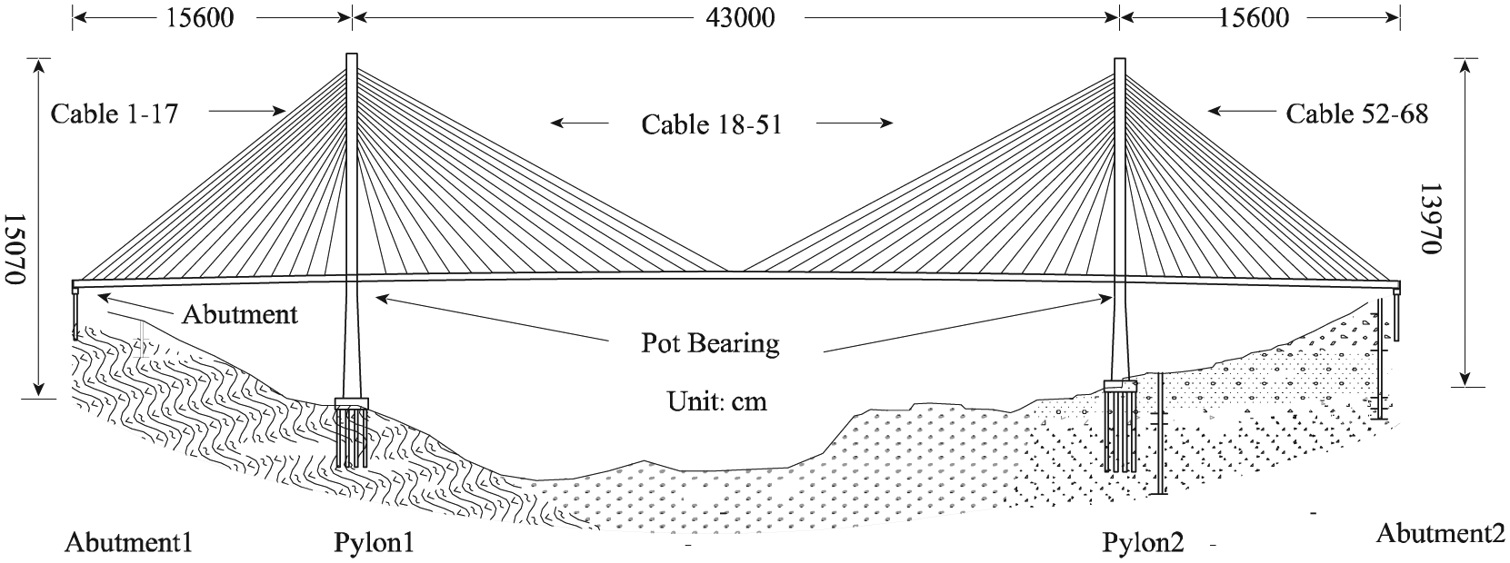
Configuration of Polonggou cable-stayed bridge.

Using the OpenSEES analysis platform (McKenna et al., 2010), which is an open source collaborative software framework for simulating the seismic response of structural and geotechnical systems, a detailed nonlinear three-dimensional model is created for the subject bridge. The superstructure is expected to remain linear and is thus modeled using elastic beam–column elements. A distributed plasticity fiber model is used to represent sections of pylons to account for the axial force–moment interaction and material nonlinearity. Each fiber is modeled with an appropriate stress–strain relationship depending on whether it represents confined concrete, unconfined concrete, or longitudinal reinforcement, as illustrated in Figure 2(d) and (e). Foundations of the pylons are modeled using six spring elements. The response of each cable is simulated using a nonlinear tension-only element, which is modeled as a large-displacement truss element using the Ernst method or modified elastic modulus method as a result of the easy usage and the capability to account for the sag effect (Pang et al., 2014). The initial stress of the cable is also considered in the model (Figure 2(d)). The abutment diagram shown in Figure 3 consists of the abutment element, the pounding element, and the bearing element. The abutment element comprising passive, active, and transverse actions is modeled by the stiffness of the passive resistance of the backfill soil (Figure 2(a)) and the stiffness of the piles (Figure 2(b)) (Choi et al., 2004; Nielson, 2005; Padgett and DesRoches, 2008). The pounding effect (Figure 2(e)) between the superstructure and abutment is modeled using the contact element approach developed by Muthukumar and DesRoches (2006), which includes hysteretic energy loss. The longitudinal response of the pot bearing (Figure 2(c)) is simulated using a nonlinear bilinear element, while the transverse response of the bearing is assumed to be constrained.

Figure 2.

Force–deformation relations of various components: (a) abutment passive, (b) abutment active, (c) pot bearing, (d) cables, and (e) pounding.

Figure 3.

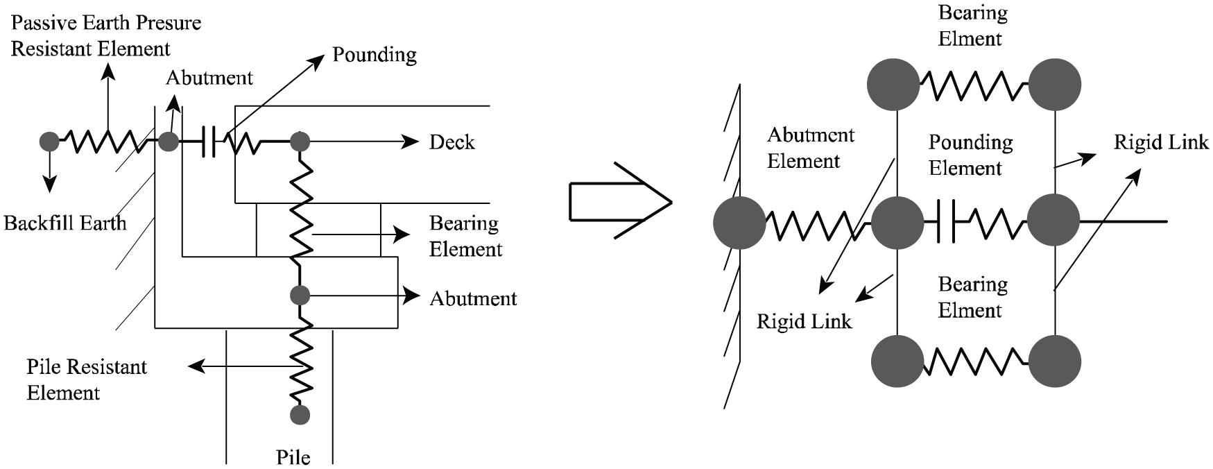
Diagram of abutments.

Uncertainty treatment

LHS approach is used to account for modeling uncertainties in the simulation of the cable-stayed bridge. Both the concrete compressive strength and rebar yield strength follow normal distribution. The compressive strength of concrete C50, which is widely used for bridges built in China, is 45.1 MPa. This value is adopted as its mean value and its coefficient of variation (COV) is 0.137. Based on the statistic, the compressive strength varies from 32.5 to 57.5 MPa for a cumulative distribution between 5% and 95%. The yielding strength of steel HRB400 can be obtained in the same way. The distribution parameters are listed in Table 1. The coefficient of friction of the pot sliding bearing is assumed to follow a uniform distribution in the range of 0.02–0.04. Rayleigh damping is used in the model but treated as a random variable. The damping ratio of concrete cable-stayed bridges is assigned as 0.03 per the Guidelines for Seismic Design of Highway Bridges in China (MOT, 2008). Thus, the damping ratio is assumed to follow the normal distribution with a mean value of 0.03 and a COV of 0.15.

Table 1.

Uncertainty parameters incorporated in analytical bridge models.

Modeling parameter	Probability distribution	Mean	COV	Units	Lower level	Upper level
Steel yield strength	Normal	435.0	0.0645	MPa	388.0	491.0
Concrete compressive strength	Normal	45.1	0.1374	MPa	32.5	57.5
Bearing coefficient of friction	Uniform	0.03	0.33	−	0.02	0.04
Passive stiffness of abutments	Uniform	20.2	0.43	kN/mm/m	11.5	28.8
Active stiffness of abutments	Uniform	16.31	0.33	kN/mm/pile	10.9	21.7
Abutment–deck gaps	Uniform	375	0.2	mm	300	450
Damping ratio	Normal	0.03	0.15	−	0.026	0.036
Deck mass (Nielson, 2007)	Uniform	1	0.1	−	0.9	1.1

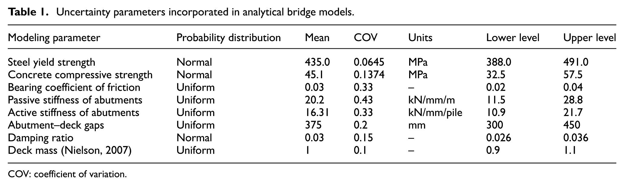
COV: coefficient of variation.

Input ground motions

This study selects the suite of ground motions used in Shafieezadeh et al. (2012), which comprises 80 ground motions extracted from the Pacific Earthquake Engineering Research Center (PEER) Strong Motion Database (Medina and Krawinkler, 2003) and 20 ground motions pertinent to Los Angeles selected from the SAC project database. The 80 PEER ground motions have an even selection of recorded time-histories from four bins that include combinations of low and high moment magnitudes as well as large and small epicentral distances. The distribution of peak ground accelerations (PGAs) related to magnitudes (M) and epicentral distance (R) is shown in Figure 4. The 20 SAC ground motions have 10 pairs with 2% and 10% probability of exceedance in 50 years. Figure 5 is the response spectra of 100 ground motions for the longitudinal and transverse directions along with the associated mean response spectrum (black line in Figure 5).

Figure 4.

Distribution of PGA related to magnitudes and epicentral distance: (a) longitudinal direction and (b) transverse direction.

Figure 5.

Response spectra of 100 ground motions: (a) longitudinal direction and (b) transverse direction.

Engineering demand parameters

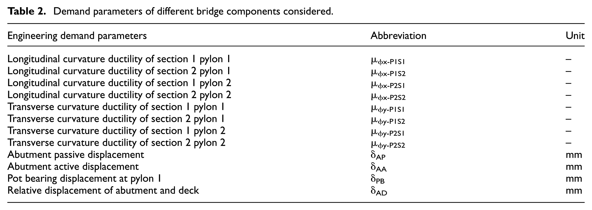
Demands placed on critical components are taken into account for the vulnerability assessment of bridges. In this study, peak demands of components are adopted as engineering demand parameters (EDPs), and the critical components are the pylons, bearings, abutments, and the relative displacement of abutment and deck, as listed in Table 2.

Table 2.

Demand parameters of different bridge components considered.

Engineering demand parameters	Abbreviation	Unit
Longitudinal curvature ductility of section 1 pylon 1	µ_ϕx-P1S1	−
Longitudinal curvature ductility of section 2 pylon 1	µ_ϕx-P1S2	−
Longitudinal curvature ductility of section 1 pylon 2	µ_ϕx-P2S1	−
Longitudinal curvature ductility of section 2 pylon 2	µ_ϕx-P2S2	−
Transverse curvature ductility of section 1 pylon 1	µ_ϕy-P1S1	−
Transverse curvature ductility of section 2 pylon 1	µ_ϕy-P1S2	−
Transverse curvature ductility of section 1 pylon 2	µ_ϕy-P2S1	−
Transverse curvature ductility of section 2 pylon 2	µ_ϕy-P2S2	−
Abutment passive displacement	δ_AP	mm
Abutment active displacement	δ_AA	mm
Pot bearing displacement at pylon 1	δ_PB	mm
Relative displacement of abutment and deck	δ_AD	mm

IM selection

Selecting an optimal IM for seismic fragility assessment is not a trivial matter and has been focused on in numerous studies (Padgett et al., 2008; Ramanathan, 2012; Shafieezadeh et al., 2012). In some of the pioneering work, various IMs were selected as optimal IM, including Modified Mercalli Intensity Scale (Applied Technology Council (ATC), 1985), PGA (Federal Emergency Management Agency (FEMA), 1997), peak ground displacement (PGD), spectral acceleration at a period of 1 s (Ramanathan, 2012), fundamental period (Sa-f) (Shome, 1999), and vector-based IMs (Baker and Cornell, 2005; Luco and Cornell, 2007).

However, almost all the optimal IM selection work was focused on highway bridges with small span lengths. The observations for highway bridges may not be applied to cable-stayed bridges because of their structural flexibility and high modal complexity. Even between different cable-stayed bridges, the optimal IM may vary. Thus, prior to performing the fragility analysis, an optimal IM should be selected for a specific cable-stayed bridge. Following the selection process proposed by Padgett et al. (2008), various optimal IM candidates are compared by examining four characteristic properties including efficiency, practicality, sufficiency, and proficiency. To determine an optimal IM, this study selects four typical IM candidates such as PGA, peak ground velocity (PGV), spectral acceleration at 0.2 s (Sa02), and Sa10.

Efficiency, practicality, and proficiency

The identification of an optimal IM can be performed using ln(IM)–ln(D) pairs obtained from a set of simulations (PSDM). An efficient IM reduces the amount of variation in the estimated demand for a given IM value (Giovenale et al., 2004). Practicality refers to whether there is any direct correlation between an IM and the seismic structure demand or not which is measured by the parameter b in equation (2).

Proficiency is a composite measure of efficiency and practicality, which is defined as

ζ = \frac{β_{D | IM}}{b}

(6)

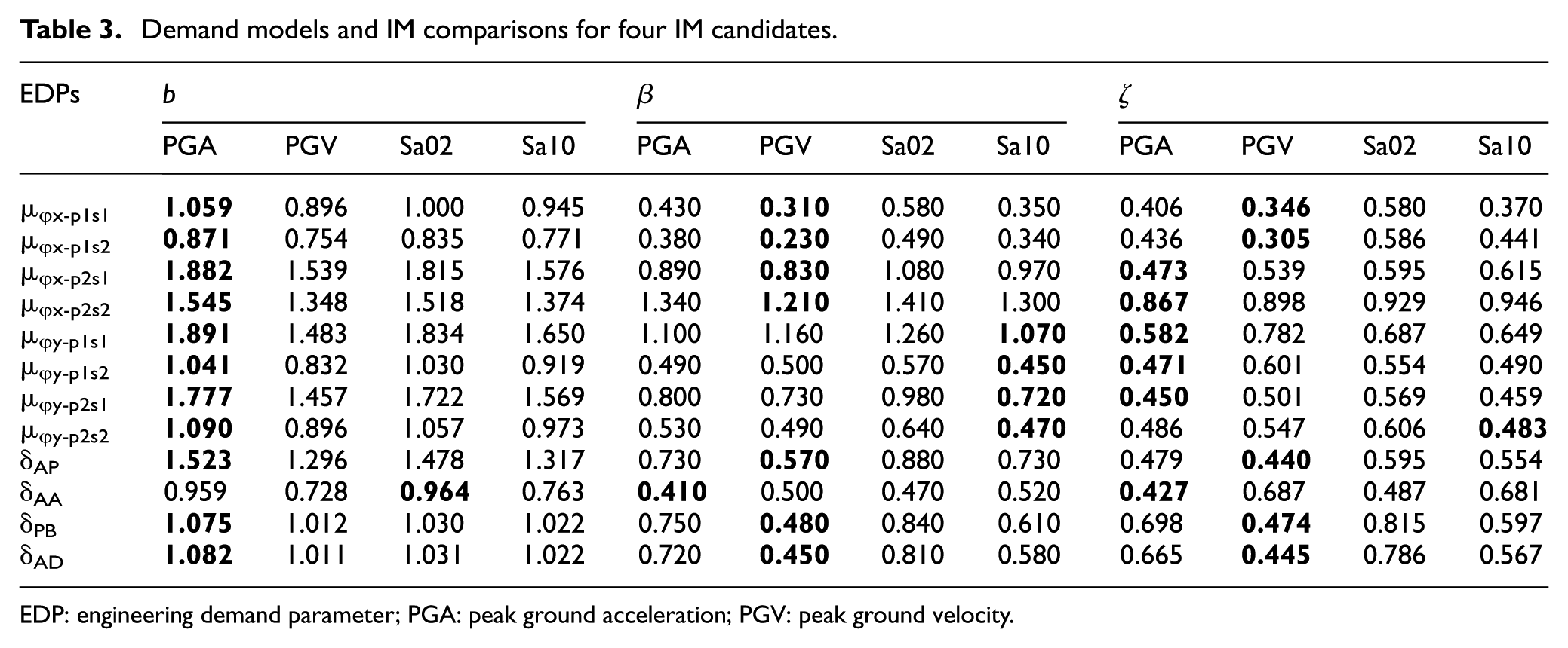
Thus, an optimal IM would be characterized by smaller values of β_D|IM and ζ and larger values of b and R². Figure 6 shows the linear regression lines of µ_ϕx-P1S1 for PGA, PGV, Sa02, and Sa10. Table 3 summarizes the characteristic properties of the four IMs for the 12 EDPs. Also, the controlling values of the aforementioned parameters b, β_D|IM, and ζ of various IMs for each EDP are highlighted in Table 3. The table reveals that PGA is the most practical IM, followed by Sa02. PGV is the most efficient IM, followed by Sa10 and Sa02 is the least efficient. Both PGA and PGV are the most proficient IMs. In conclusion, PGA and PGV tend to be the optimal IMs in terms of efficiency, practicality, and proficiency.

Figure 6.

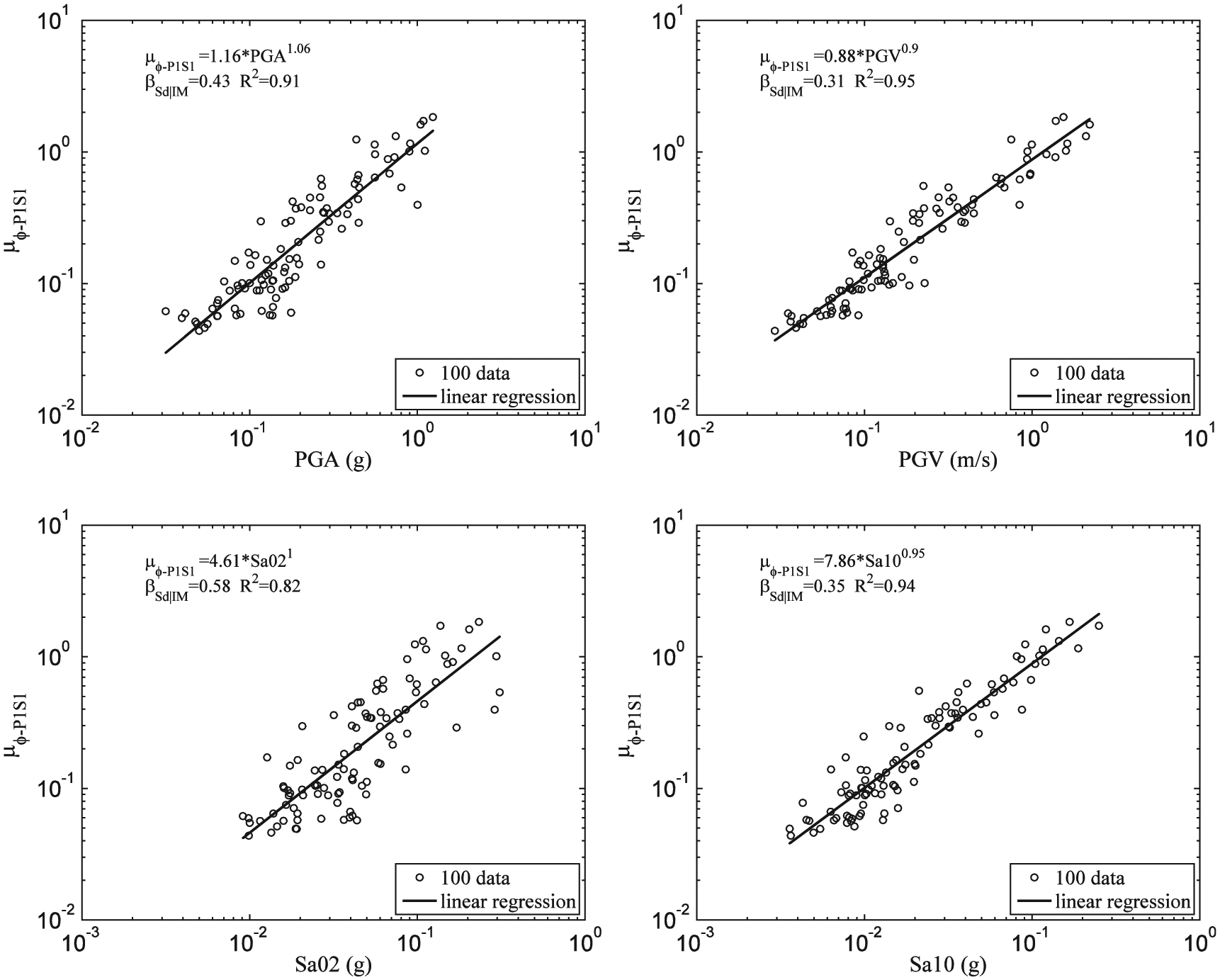
Probabilistic seismic demand models for PGA, PGV, Sa02, and Sa10.

Table 3.

Demand models and IM comparisons for four IM candidates.

EDPs	b				β				ζ
EDPs	PGA	PGV	Sa02	Sa10	PGA	PGV	Sa02	Sa10	PGA	PGV	Sa02	Sa10
µ_φx-p1s1	1.059	0.896	1.000	0.945	0.430	0.310	0.580	0.350	0.406	0.346	0.580	0.370
µ_φx-p1s2	0.871	0.754	0.835	0.771	0.380	0.230	0.490	0.340	0.436	0.305	0.586	0.441
µ_φx-p2s1	1.882	1.539	1.815	1.576	0.890	0.830	1.080	0.970	0.473	0.539	0.595	0.615
µ_φx-p2s2	1.545	1.348	1.518	1.374	1.340	1.210	1.410	1.300	0.867	0.898	0.929	0.946
µ_φy-p1s1	1.891	1.483	1.834	1.650	1.100	1.160	1.260	1.070	0.582	0.782	0.687	0.649
µ_φy-p1s2	1.041	0.832	1.030	0.919	0.490	0.500	0.570	0.450	0.471	0.601	0.554	0.490
µ_φy-p2s1	1.777	1.457	1.722	1.569	0.800	0.730	0.980	0.720	0.450	0.501	0.569	0.459
µ_φy-p2s2	1.090	0.896	1.057	0.973	0.530	0.490	0.640	0.470	0.486	0.547	0.606	0.483
δ_AP	1.523	1.296	1.478	1.317	0.730	0.570	0.880	0.730	0.479	0.440	0.595	0.554
δ_AA	0.959	0.728	0.964	0.763	0.410	0.500	0.470	0.520	0.427	0.687	0.487	0.681
δ_PB	1.075	1.012	1.030	1.022	0.750	0.480	0.840	0.610	0.698	0.474	0.815	0.597
δ_AD	1.082	1.011	1.031	1.022	0.720	0.450	0.810	0.580	0.665	0.445	0.786	0.567

EDP: engineering demand parameter; PGA: peak ground acceleration; PGV: peak ground velocity.

Sufficiency

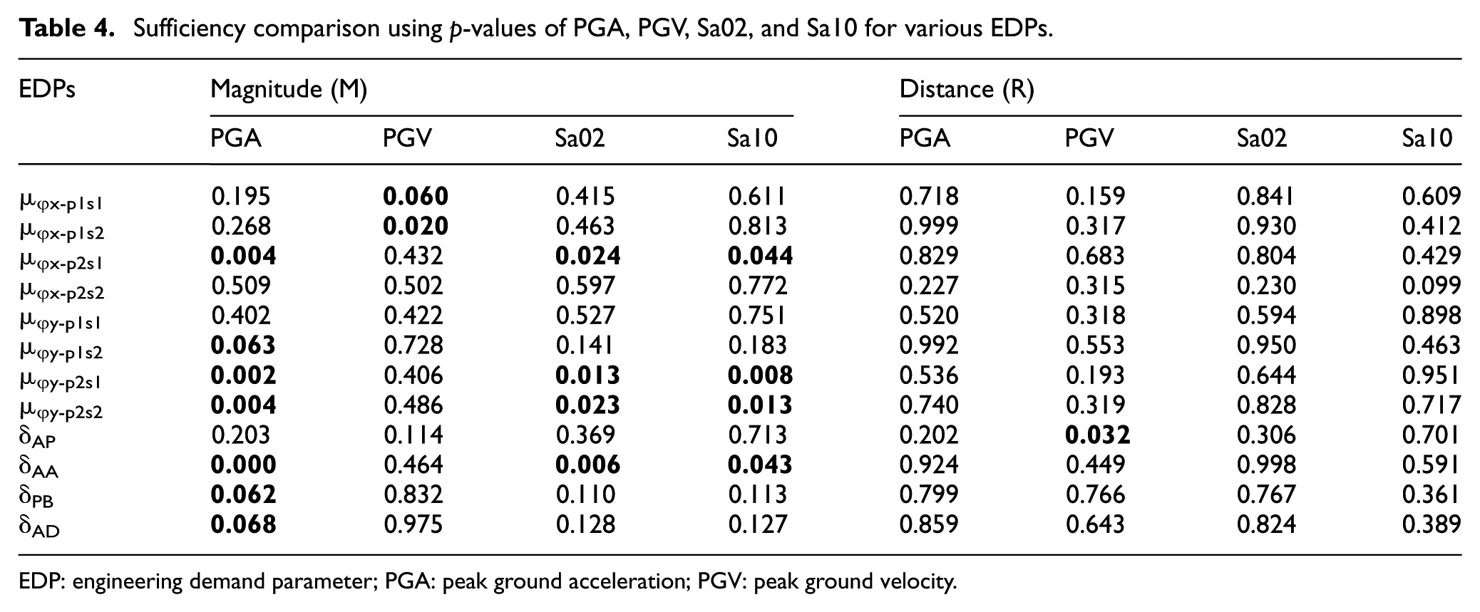
Sufficiency refers to the property where an IM is independent of ground motion characteristics such as magnitude (M) and epicentral distance (R). The sufficiency of an IM is evaluated by performing a regression analysis on the residuals ( $ε | IM = \ln (d_{i}) - [\ln (a) + b \ln (IM)]$ ) from the PSDM relative to the ground motion characteristic, M or R. The null hypothesis is that the coefficient of regression is 0 (the IM is independent of M or R). Larger p-values imply stronger evidence for accepting the null hypothesis and evidence of sufficient IM. Smaller p-values (the cutoff is considered as 0.1) indicate that IM is dependent on the M or R. Table 4 presents the p-values for PGA, PGV, Sa02, and Sa10. In the table, the p-values less than 0.1 are highlighted. In general, the majority of the IMs are independent of R. However, the IMs are examined to be less sufficient with respect to M. Seven EDPs (µ_φx-p2s1, µ_φy-p1s2, µ_φy-p2s1, µ_φy-p2s2, δ_AA, δ_PB, and δ_AD) conditioned on PGA are dependent on M (with the p-values less than 0.1), while two EDPs conditioned on PGV depend on M. Thus, PGV is more sufficient than PGV. Therefore, PGV is the most efficient, proficient, and sufficient IM among the four IMs for the cable-stayed bridge. Therefore, PGV is selected as the optimal IM for this study (Figure 7).

Table 4.

Sufficiency comparison using p-values of PGA, PGV, Sa02, and Sa10 for various EDPs.

EDPs	Magnitude (M)				Distance (R)
EDPs	PGA	PGV	Sa02	Sa10	PGA	PGV	Sa02	Sa10
µ_φx-p1s1	0.195	0.060	0.415	0.611	0.718	0.159	0.841	0.609
µ_φx-p1s2	0.268	0.020	0.463	0.813	0.999	0.317	0.930	0.412
µ_φx-p2s1	0.004	0.432	0.024	0.044	0.829	0.683	0.804	0.429
µ_φx-p2s2	0.509	0.502	0.597	0.772	0.227	0.315	0.230	0.099
µ_φy-p1s1	0.402	0.422	0.527	0.751	0.520	0.318	0.594	0.898
µ_φy-p1s2	0.063	0.728	0.141	0.183	0.992	0.553	0.950	0.463
µ_φy-p2s1	0.002	0.406	0.013	0.008	0.536	0.193	0.644	0.951
µ_φy-p2s2	0.004	0.486	0.023	0.013	0.740	0.319	0.828	0.717
δ_AP	0.203	0.114	0.369	0.713	0.202	0.032	0.306	0.701
δ_AA	0.000	0.464	0.006	0.043	0.924	0.449	0.998	0.591
δ_PB	0.062	0.832	0.110	0.113	0.799	0.766	0.767	0.361
δ_AD	0.068	0.975	0.128	0.127	0.859	0.643	0.824	0.389

EDP: engineering demand parameter; PGA: peak ground acceleration; PGV: peak ground velocity.

Figure 7.

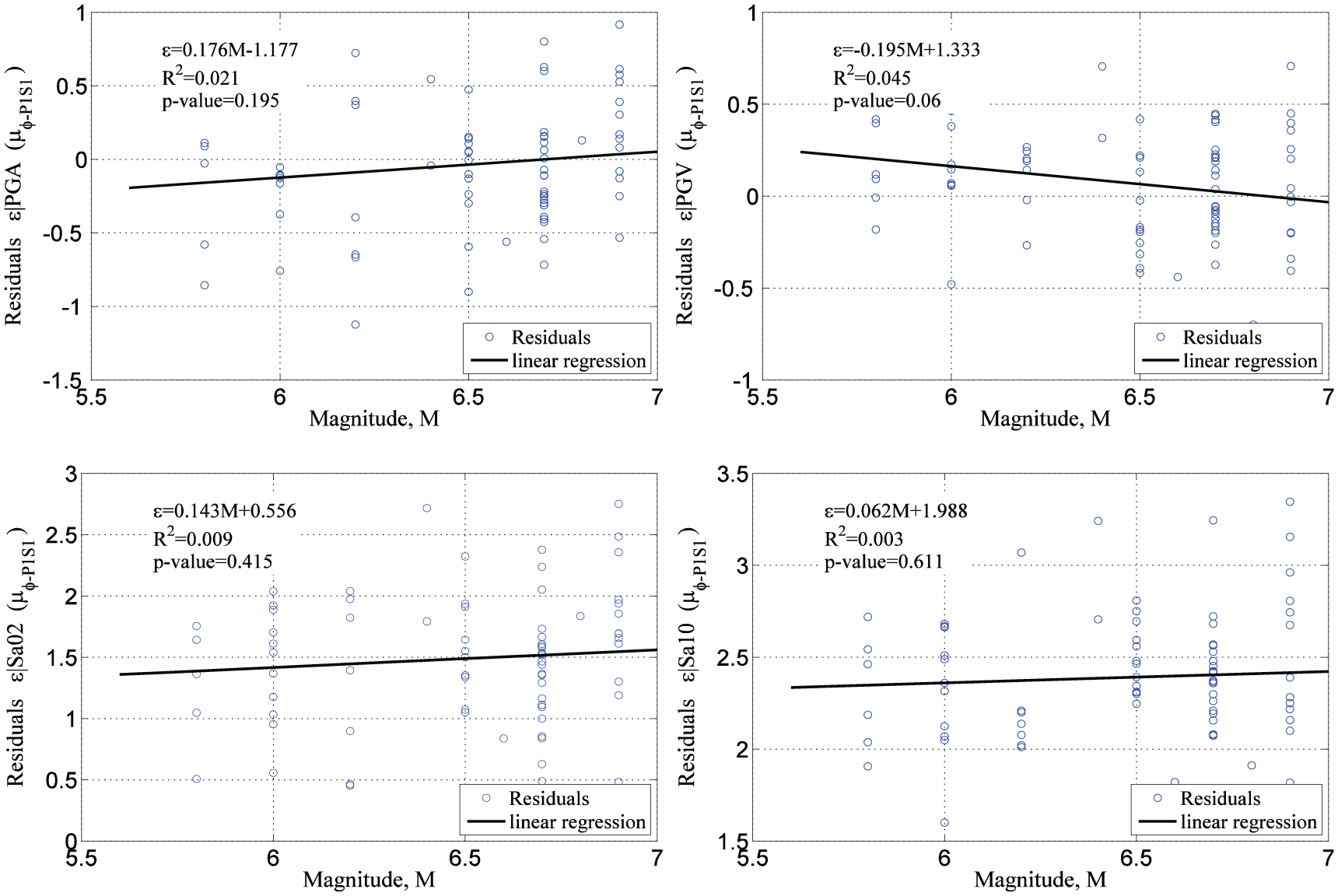
Comparison of the sufficiency of four IMs for µ_ϕx-p1s1 by examining the conditional statistical independence from magnitude.

Component classification and limit state definition

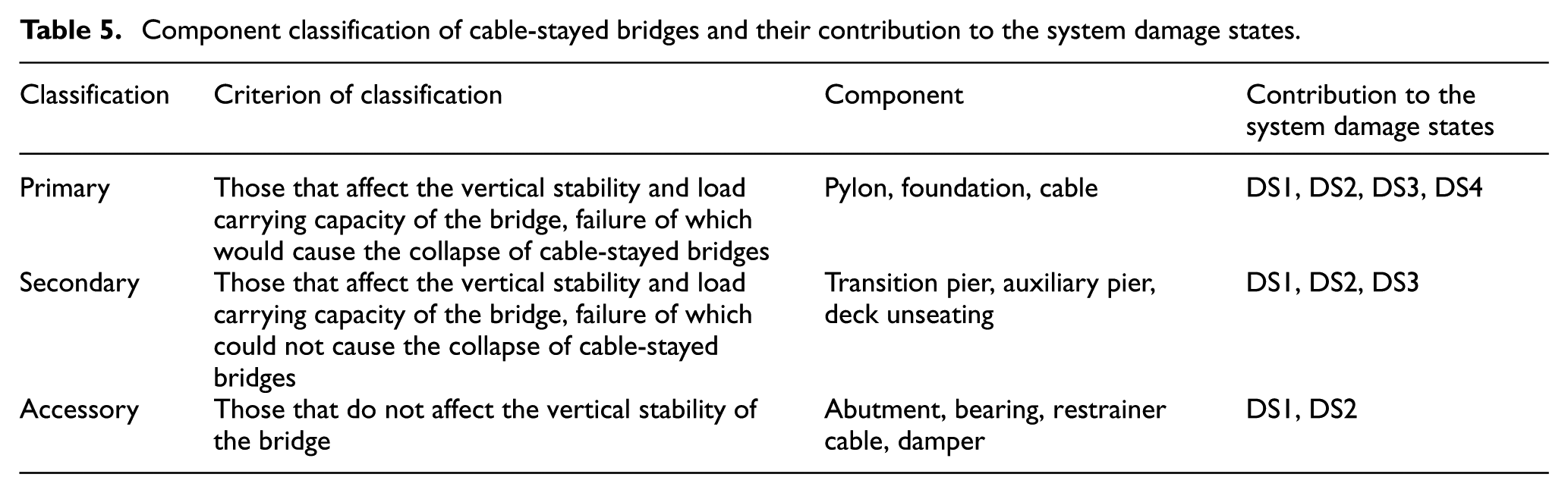
Ramanathan (2012) derives limit states for various components of highway bridges compatible with the California Department of Transportation (Caltrans) seismic design code (Caltrans, 1999) and operational experience. The limit state facilitates the evaluation of repair-related decision variables (repair cost and repair time), which are the final products in a regional risk assessment procedure. Learning from the component classification for buildings by Structural Engineers Association of California (SEAOC, 1995), FEMA (1996), ACT (2006), and for highway bridges by Ramanathan (2012), the classification of components in cable-stayed bridges is proposed in this study. The components are considered as primary, secondary, or accessory, which are indicated in Table 5. The superstructure unseating is regarded as a primary component in ordinary highway bridges while it is referred to as a secondary component in cable-stayed bridges because its local failure would not be expected to cause the collapse of cable-stayed bridges. In the table, DS1–DS4 represent the slight, moderate, extensive, and complete damage state, respectively.

Table 5.

Component classification of cable-stayed bridges and their contribution to the system damage states.

Classification	Criterion of classification	Component	Contribution to the system damage states
Primary	Those that affect the vertical stability and load carrying capacity of the bridge, failure of which would cause the collapse of cable-stayed bridges	Pylon, foundation, cable	DS1, DS2, DS3, DS4
Secondary	Those that affect the vertical stability and load carrying capacity of the bridge, failure of which could not cause the collapse of cable-stayed bridges	Transition pier, auxiliary pier, deck unseating	DS1, DS2, DS3
Accessory	Those that do not affect the vertical stability of the bridge	Abutment, bearing, restrainer cable, damper	DS1, DS2

As seen in equation (1), the fragility function requires capacity-based limit state models representing the extent of damage on structural component or system. This study partially employs the existing models or definitions of limit states used in previous studies. The limit states for the abutments follow the work of Ramanathan (2012). The design displacement of the pot bearing is ±300 mm. Thus, two limit states are defined for the pot bearing: LS1 is 300 mm and LS2 is 600 mm. Limit states for the abutment seat are intimately linked to the unseating of superstructure. This study uses the moderate (LS₂) and extensive (LS₃) limit states for the abutment seat determined per the definition of Avşar et al. (2011), which is illustrated in Figure 8. Table 6 lists the values of limit states for the above-mentioned components. The LS3 and LS4 of the abutment and bearing are not defined because these components are regarded as accessory components, and thus contribute only to the slight and moderate damages of cable-stayed bridges.

Figure 8.

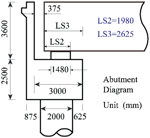
Limit states of abutment seat.

Table 6.

Limit state models for various EDPs.

EDPs	LS1		LS2		LS3		LS4
EDPs	S_C	β_C	S_C	β_C	S_C	β_C	S_C	β_C
µ_φx-p1s1	1.00	0.35	1.33	0.35	4.52	0.35	24.8	0.35
µ_φx-p1s2	1.00	0.35	−	−	1.37	0.35	6.27	0.35
µ_φx-p2s1	1.00	0.35	1.33	0.35	4.52	0.35	24.8	0.35
µ_φx-p2s2	1.00	0.35	−	−	1.37	0.35	6.27	0.35
µ_φy-p1s1	1.00	0.35	1.17	0.35	4.57	0.35	24.4	0.35
µ_φy-p1s2	1.00	0.35	−	−	1.33	0.35	4.9	0.35
µ_φy-p2s1	1.00	0.35	1.17	0.35	4.57	0.35	24.4	0.35
µ_φy-p2s2	1.00	0.35	−	−	1.33	0.35	4.9	0.35
δ_AP	48.8	0.35	170.8	0.35	−	−	−	−
δ_AA	46.5	0.35	155.0	0.35	−	−	−	−
δ_PB	300	0.10	600	0.10		−	−	−
δ_AD	−	−	1980	0.10	2625	0.10	−	−

EDP: engineering demand parameter.

The column is the most critical component of bridges when performing the fragility analysis of the highway bridges. Several previous studies (Nielson and DesRoches, 2007; Pan et al., 2007; Ramanathan, 2012; Zhang and Huo, 2009) defined different limit states for columns and achieved different conclusions. However, the limit states are related to the geometry of the section, material, volumetric percentage of the confining steel, and axial compression ratio (ACR) of the section. Due to the large geometric size and high ACR of the pylon section, there exists a great difference in the section capacity between the column of highway bridges and pylon of cable-stayed bridges. Thus, it is necessary to define the limit states for each section of interest of the pylon.

First, a fiber section is created using OpenSEES (McKenna et al., 2010), and a pushover analysis is then performed to obtain the moment–curvature curve of the section. Following the flow chart shown in Figure 9, various limit states for the pylon section are determined.

Figure 9.

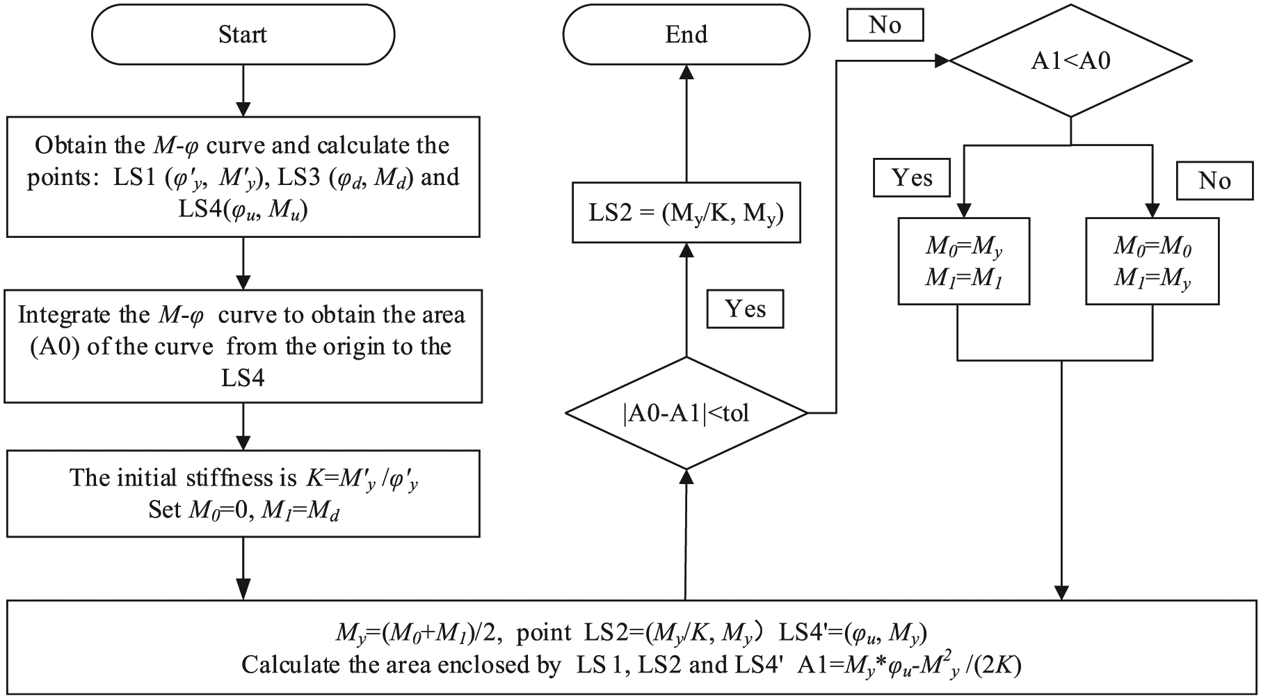
Flow chart to determine the limit states of the pylon section: (a) along transverse direction and (b) along longitudinal direction.

The Kent–Scott–Part model (Park and Paulay, 1975; Scott et al., 1982) is employed to simulate the C50 (MOT, 2008) concrete of the fiber section in this study (Figure 10(c)). For the confined concrete, the crushing strain and corresponding stress of the core concrete are $ε_{cu}$ and $0.2 K f'_{c}$ , respectively. The ultimate stress and the corresponding strain are $K f'_{c}$ and 0.002 K, respectively. Here, $K = 1 + ρ_{s} f_{yh} / f'_{c}$ and $ε_{cu} = 0.004 + 0.9 ρ_{s} f_{yh} / 300$ . $ρ_{t}$ is the volumetric ratio of the stirrup, $f_{yh}$ is the yield strength of the stirrup, and $f'_{c}$ is the compressive strength of the cover concrete.

Figure 10.

Configuration and fiber model of the pylons of cable-stayed bridge (cm): (a) configuration of pylons, (b) fiber section of sections 1 and 2, (c) force–deformation relationship of core and cover concrete and (d) force–deformation relationship of longitudinal bar.

Figure 10(b) illustrates the structural geometry of sections 1 and 2. L1 and W1 are the length and width, respectively, of the outside of the section; L2 and W2 represents the length and width, respectively, of the hole inside the section. The ACR is designed as 0.235 for section 1 and 0.35 for section 2. HRB335 (MOT, 2008) is used as the stirrup and the volumetric stirrup ratio ( $ρ_{t}$ ) is 1.2%. HRB400 (MOT, 2008) is used as the longitudinal rebar and the longitudinal reinforcement ratio ( $ρ_{l}$ ) is 1.5.

Four different limit states for the curvature ductility of the pylon sections are determined following the descriptions in Table 7. As presented in the table, LS1, LS3, and LS4 can be easily derived from the pushover analysis results for the fiber section. The state of LS2 corresponding to the moderate damage state is calculated by the equal area rule based on the Guideline for Seismic Design of Highway Bridges (MOT, 2008), which is outlined in Figure 9. Figures 11 and 12 depict the moment (M)–curvature (φ) curves generated by the pushover analyses and associated equivalent bilinear curves, respectively. The curvature at the turning point of the bilinear curves (marked as φ₁ in the figures) is the limit state corresponding to the moderate damage. Comparison of the M–φ curves of sections 1 and 2 indicates that the curvature of section 1 with two holes and an ACR of 23.5% is much larger than that of section 2 with one hole and an ACR of 35%. For section 2, the plastic hinge is formed before the first yield of reinforcing rebars due to the higher ACR, which is not true in reality. Thus, only three limit states are defined for section 2 (φ₁, φ₃, and φ₄,) along the longitudinal and transverse directions. The normalized values of the curvature with respect to φ₁ are listed in Table 6.

Table 7.

Physical description of limit states of curvature ductility of pylon section.

Limit state	Slight damage, φ₁	Moderate damage, φ₂	Extensive damage, φ₃	Complete damage, φ₄
Description	First yield of reinforcing bars	Formation of plastic hinge in the column	Ultimate stress of corner concrete	Crushing of corner concrete

Figure 11.

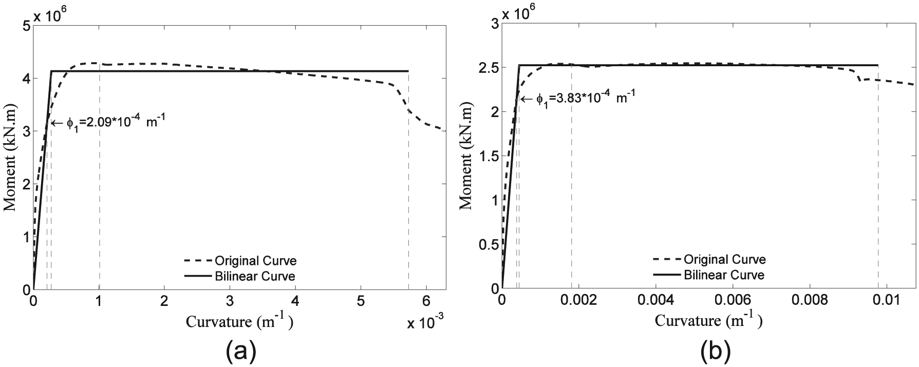
M–φ curves and limit states of pylon section 1: (a) along transverse direction and (b) along longitudinal direction.

Figure 12.

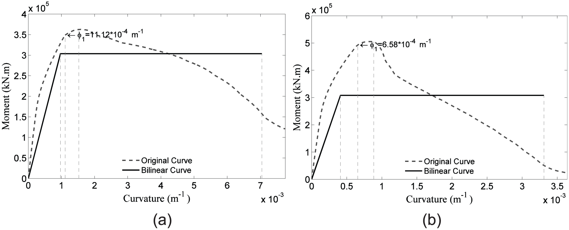
M–φ curves and limit states of pylon section 2: (a) along transverse direction and (b) along longitudinal direction.

Bridge component fragility

Using the PSDM and the limit states in the framework of equation (1), fragility curves for each of bridge components are easily calculated and plotted in Figure 13. The pot bearing (δ_PB) appears to be the most vulnerable component at the slight damage state, followed by the abutments (δ_AP and δ_AA). For the moderate damage state, the pot bearing (δ_PB) is still the most vulnerable component, but followed by section 1 of pylon 2 (µ_φx-p2s1). However, section 2 of pylon 2 (µ_φx-p2s2) and section 1 of pylon 2 (µ_φx-p2s1) are the most vulnerable components at the extensive damage state and complete damage state, respectively. For all the damage states, pylon 2 is more vulnerable than pylon 1. This is associated with the fact that pylon 1 is longer and more flexible than pylon 2, and thus, pylon 2 experiences larger seismic demands than pylon 1. Additionally, section 1 for both pylons is more vulnerable than section 2 for the longitudinal direction, but less vulnerable for the transverse direction.

Figure 13.

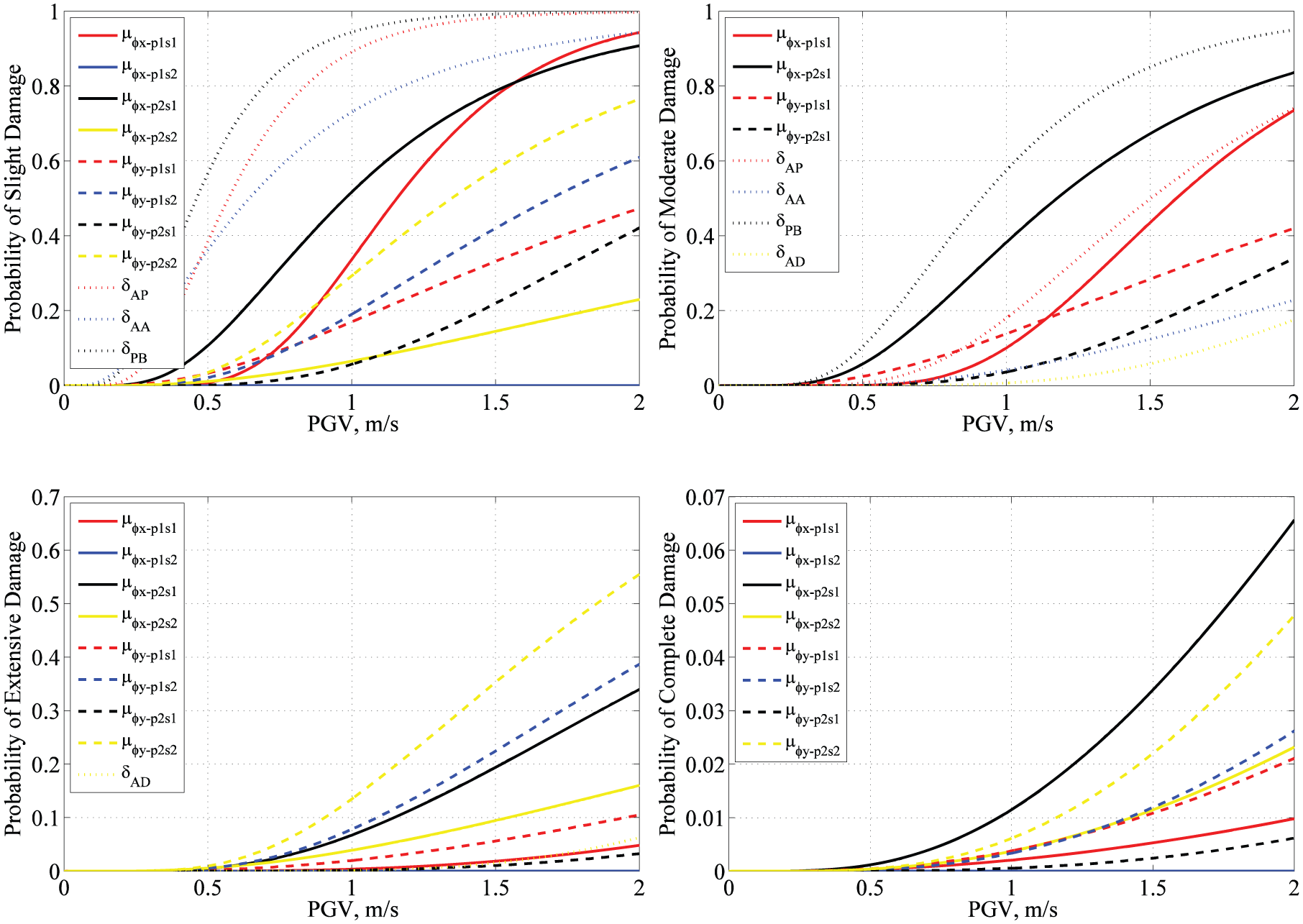
Component fragility curves for the cable-stayed bridge.

Bridge system fragility

X = (X₁, X₂,…, X₁₂) represents the vector of demands, placed on the EDPs of the cable-stayed bridge, and Y = ln(X) is the vector of demands in the log-transformed space. JPSDM is then formulated in the log-transformed space by assembling the vector of means $μ_{Y} (PGV = pgv)$ and the covariance matrix $σ_{Y}$ . The correlation coefficient matrix of the demand of 12 EDPs is listed in Table 8. MCS is used to compare realizations of the demand and capacity of components to calculate the failure probability of the system using equation (5). Finally, a system fragility curve can be determined as a lognormal cumulative distribution function with two parameters (median and dispersion) by performing a regression analysis (hereafter, called MCS-based system fragility curve). Assuming the bridges as a serial system, the upper and lower bounds of the bridge system can be calculated in equation (7)

max [F r_{i}] ⩽ F r_{system} = ⋃_{i = 1}^{n} F r_{i} ⩽ 1 - Π_{i = 1}^{n} [1 - Fr (i)]

(7)

where Fr_i is the failure probability of the ith component and Fr_system is the failure probability of the system. The upper bound of the system fragility curves means full relevant of the components, while the lower bound means completely irrelevant of the components. Thus, the lower bound is associated with the fragility of the most vulnerable component.

Table 8.

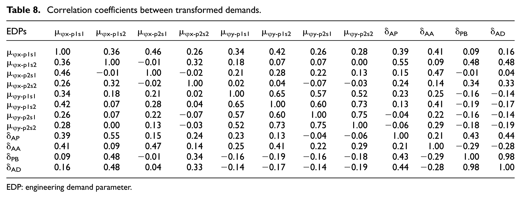
Correlation coefficients between transformed demands.

EDPs	µ_φx-p1s1	µ_φx-p1s2	µ_φx-p2s1	µ_φx-p2s2	µ_φy-p1s1	µ_φy-p1s2	µ_φy-p2s1	µ_φy-p2s2	δ_AP	δ_AA	δ_PB	δ_AD
µ_φx-p1s1	1.00	0.36	0.46	0.26	0.34	0.42	0.26	0.28	0.39	0.41	0.09	0.16
µ_φx-p1s2	0.36	1.00	−0.01	0.32	0.18	0.07	0.07	0.00	0.55	0.09	0.48	0.48
µ_φx-p2s1	0.46	−0.01	1.00	−0.02	0.21	0.28	0.22	0.13	0.15	0.47	−0.01	0.04
µ_φx-p2s2	0.26	0.32	−0.02	1.00	0.02	0.04	−0.07	−0.03	0.24	0.14	0.34	0.33
µ_φy-p1s1	0.34	0.18	0.21	0.02	1.00	0.65	0.57	0.52	0.23	0.25	−0.16	−0.14
µ_φy-p1s2	0.42	0.07	0.28	0.04	0.65	1.00	0.60	0.73	0.13	0.41	−0.19	−0.17
µ_φy-p2s1	0.26	0.07	0.22	−0.07	0.57	0.60	1.00	0.75	−0.04	0.22	−0.16	−0.14
µ_φy-p2s2	0.28	0.00	0.13	−0.03	0.52	0.73	0.75	1.00	−0.06	0.29	−0.18	−0.19
δ_AP	0.39	0.55	0.15	0.24	0.23	0.13	−0.04	−0.06	1.00	0.21	0.43	0.44
δ_AA	0.41	0.09	0.47	0.14	0.25	0.41	0.22	0.29	0.21	1.00	−0.29	−0.28
δ_PB	0.09	0.48	−0.01	0.34	−0.16	−0.19	−0.16	−0.18	0.43	−0.29	1.00	0.98
δ_AD	0.16	0.48	0.04	0.33	−0.14	−0.17	−0.14	−0.19	0.44	−0.28	0.98	1.00

EDP: engineering demand parameter.

Figure 14 compares the upper and lower bound fragility curves and MCS-based fragility curves of the bridge system for four limit states. The MCS-based system fragility curve lies in the upper and lower bounds, but much closer to the upper bound fragility curve. This is mainly due to the fact that the correlation coefficients between the transformed demands of components are small, as listed in Figure 5. The median value of the MCS-based, lower bound, and upper bound fragility curves of the bridge system is calculated and presented in Table 9. This table also presents the percentage difference between the median values of the lower or upper bound fragility curves and MCS-based fragility curves. As expected, the percentage difference between the median values of MCS-based and upper bound fragility curves is much smaller due to the small correlation coefficients.

Figure 14.

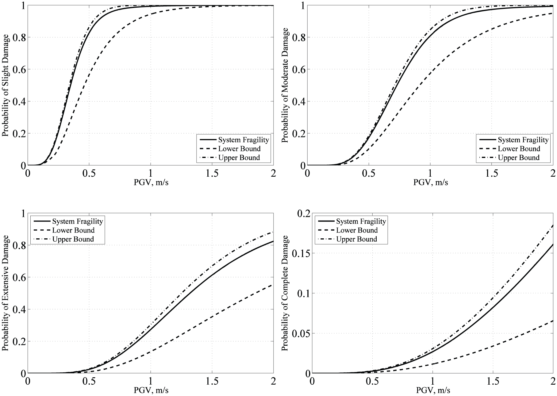
Comparison of system fragility curves for four different limit states.

Table 9.

Comparison of the median value (PGV) of the MCS-based, lower, and upper bound fragility curves for the bridge system.

Damage state	MCS-based	Lower bound		Upper bound
Damage state	Median (m/s)	Median (m/s)	Difference (%)	Median (m/s)	Difference (%)
Slight damage	0.35	0.47	34.3	0.34	2.9
Moderate damage	0.73	0.92	26.0	0.71	2.7
Extensive damage	1.33	1.86	39.8	1.26	5.3
Complete damage	3.92	7.87	100.8	3.53	9.9

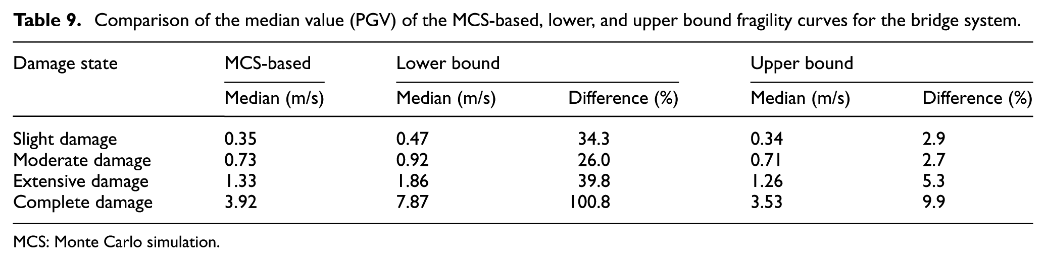
MCS: Monte Carlo simulation.

Conclusion

This study presents an analytical method to formulate component and system fragility curves of long-span cable-stayed bridges. The analytical method includes the selection of the optimal IM and the definition of limit states of various components, which are compatible with long-span cable-stayed bridges. All major components are taken into account to obtain the system fragility of cable-stayed bridges using JPSDMs and MCS. To achieve this goal, this study selects Polonggou cable-stayed bridge located in Sichuan, China, as a case-study. A set of numerical bridge models are probabilistically generated in OpenSEES by accounting for the uncertainty in the material properties. To determine an optimal IM for this subject bridge, four typical IM candidates (PGA, PGV, Sa02, and Sa10) are selected and are compared by examining four characteristic properties including efficiency, practicality, sufficiency, and proficiency. This comparison indicates that PGV is the most efficient, proficient, and sufficient IM among four IM candidates for the cable-stayed bridge. Additionally, the limit state model of the components except for pylons is modified using the existing models and model definitions used in previous studies. Due to the limitation of experimental data and expert opinion for the pylons, their limit state models in terms of curvature ductility are defined using a pushover analysis and idealized bilinear fitting. The ductility of section 1 with two holes and an ACR of 23.5% is much larger than that of section 2 with one hole and an ACR of 35%. For section 2, the plastic hinge is formed before the first yield of rebars due to the higher ACR, and thus, only three limit states are defined.

Using the demand models based on optimal IM and limit state models, component fragility curves of the cable-stayed bridge are developed and then its system fragility curves are derived using joint probabilistic demand models and MCS. The pot bearing is the most vulnerable component at the slight and moderate damage states. Section 2 and section 1 of pylon 2 are the most vulnerable component at the extensive and complete damage state, respectively. Pylon 2 is more vulnerable than pylon 1 due to its higher stiffness. Section 1 for both pylons is more vulnerable than section 2 for the longitudinal direction, but less vulnerable for the transverse direction. In addition to the MCS-based system fragility functions, the upper and lower bound fragility curves are computed assuming no and full correlation, respectively, between seismic demands of various components. The accurate (MCS-based) system fragility is formulated by considering actual correlation coefficients between them. The results show that the percentage difference between the accurate and upper bound fragilities is much smaller than that between the accurate and lower bound fragilities as a result of small correlation coefficients.

Footnotes

Declaration of Conflicting Interests

The author(s) declared no potential conflicts of interest with respect to the research, authorship, and/or publication of this article.

Funding

The author(s) disclosed receipt of the following financial support for the research, authorship, and/or publication of this article: This study was supported by State Key Laboratory of Disaster Reduction in Civil Engineering under Grant No. SLDRCE14-B-14; the National Natural Science Foundation of China under Grant Nos 51478339, 51278376, and 91315301; and Science Technology Plan of JiangXi Province under Grant No. 20151BBG70064. The supports are gratefully acknowledged.

References

Applied Technology Council (ATC) (1985) Earthquake Damage Evaluation Data for California. Redwood City, CA: ATC.

Applied Technology Council (ATC) (2006) FEMA 445. Next-Generation Performance-Based Seismic Design Guidelines—Program Plan for New and Existing Buildings. Redwood City, CA: ATC.

Avşar

Yakut

Caner

(2011) Analytical fragility curves for ordinary highway bridges in Turkey. Earthquake Spectra 27(4): 971–996.

Baker

Cornell

(2005) A vector-valued ground motion intensity measure consisting of spectral acceleration and epsilon. Earthquake Engineering & Structural Dynamics 34(10): 1193–1217.

Barnawi

Dyke

(2013) Seismic fragility relationships of a cable-stayed bridge equipped with response modification systems. Journal of Bridge Engineering 19: A4013003.

Basoz

Kiremidjian

King

. (1999) Statistical analysis of bridge damage data from the 1994 Northridge, CA, earthquake. Earthquake Spectra 15(1): 25–54.

California Department of Transportation (Caltrans) (1999) Caltrans Seismic Design Criteria. Sacramento, CA: (Caltrans).

Casciati

Cimellaro

Domaneschi

(2008) Seismic reliability of a cable-stayed bridge retrofitted with hysteretic devices. Computers & Structures 86(17–18): 1769–1781.

Choi

DesRoches

Nielson

(2004) Seismic fragility of typical bridges in moderate seismic zones. Engineering Structures 26(2): 187–199.

10.

Cornell

Jalayer

Hamburger

. (2002) Probabilistic basis for 2000 SAC Federal Emergency Management Agency steel moment frame guidelines. Journal of Structural Engineering: ASCE 128(4): 526–533.

11.

Federal Emergency Management Agency (FEMA) (1996) FEMA 273. NEHRP Guidelines for the Seismic Rehabilitation of Buildings. Washington, DC: FEMA.

12.

Federal Emergency Management Agency (FEMA) (1997) FEMA 274. NEHRP Commentary on the Guidelines for the Seismic Rehabilitation of Buildings. Washington, DC: FEMA.

13.

Giovenale

Cornell

Esteva

(2004) Comparing the adequacy of alternative ground motion intensity measures for the estimation of structural responses. Earthquake Engineering & Structural Dynamics 33(8): 951–979.

14.

Hwang

Liu

Chiu

(2001) Seismic Fragility Analysis of Highway Bridges. Memphis, TN: MAEC, Center for Earthquake Research and Information, The University of Memphis.

15.

Luco

Cornell

(2007) Structure-specific scalar intensity measures for near-source and ordinary earthquake ground motions. Earthquake Spectra 23(2): 357–392.

16.

McKenna

Scott

Fenves

(2010) Nonlinear finite-element analysis software architecture using object composition. Journal of Computing in Civil Engineering 24(1): 95–107.

17.

Mackie

Stojadinovic

(2001) Probabilistic seismic demand model for California highway bridges. Journal of Bridge Engineering 6(6): 468–481.

18.

Medina

Krawinkler

(2003) Seismic Demands for Nondeteriorating Frame Structures and Their Dependence on Ground Motions. Stanford, CA: The John A. Blume Earthquake Engineering Center, Stanford University.

19.

MOT (2008) Guidelines for Seismic Design of Highway Bridges. Beijing, China: MOT.

20.

Muthukumar

DesRoches

(2006) A Hertz contact model with non-linear damping for pounding simulation. Earthquake Engineering & Structural Dynamics 35(7): 811–828.

21.

Nielson

(2005) Analytical fragility curves for highway bridges in moderate seismic zones. PhD Dissertation, Georgia Institute of Technology, Atlanta, GA.

22.

Nielson

DesRoches

(2007) Seismic fragility methodology for highway bridges using a component level approach. Earthquake Engineering & Structural Dynamics 36(6): 823–839.

23.

Padgett

DesRoches

(2008) Methodology for the development of analytical fragility curves for retrofitted bridges. Earthquake Engineering & Structural Dynamics 37(8): 1157–1174.

24.

Padgett

Nielson

DesRoches

(2008) Selection of optimal intensity measures in probabilistic seismic demand models of highway bridge portfolios. Earthquake Engineering & Structural Dynamics 37(5): 711–725.

25.

Pan

Agrawal

Ghosn

(2007) Seismic fragility of continuous steel highway bridges in New York state. Journal of Bridge Engineering 12(6): 689–699.

26.

Pang

Shen

. (2014) Seismic fragility analysis of cable-stayed bridges considering different sources of uncertainties. Journal of Bridge Engineering 19(4): 04013015.

27.

Park

Paulay

(1975) Reinforced Concrete Structures. New York: Wiley.

28.

Ramanathan

(2012) Next generation seismic fragility curves for California bridges incorporating the evolution in seismic design. PhD Dissertation, Georgia Institute of Technology, Atlanta, GA.

29.

Ren

Obata

(1999) Elastic-plastic seismic behavior of long span cable-stayed bridges. Journal of Bridge Engineering 4(3): 194–203.

30.

Scott

Park

Priestley

(1982) Stress-strain behavior of concrete confined by overlapping hoops at low and high strain rates. ACI Structural Journal 79(6): 13–27.

31.

Shafieezadeh

Ramanathan

Padgett

. (2012) Fractional order intensity measures for probabilistic seismic demand modeling applied to highway bridges. Earthquake Engineering & Structural Dynamics 41(3): 391–409.

32.

Shinozuka

Feng

Kim

. (2000a) Nonlinear static procedure for fragility curve development. Journal of Engineering Mechanics: ASCE 126(12): 1287–1295.

33.

Shinozuka

Feng

Lee

. (2000b) Statistical analysis of fragility curves. Journal of Engineering Mechanics: ASCE 126(12): 1224–1231.

34.

Shome

(1999) Probabilistic Seismic Demand Analysis of Non-linear Structures. Ph.D. Thesis, Stanford University.

35.

Structural Engineers Association of California (SEAOC) (1995) Vision 2000: Conceptual Frame Work for Performance-Based Seismic Design. Sacramento, CA: SEAOC.

36.

Zhang

Huo

(2009) Evaluating effectiveness and optimum design of isolation devices for highway bridges using the fragility function method. Engineering Structures 31(8): 1648–1660.