Model test for the tensioning construction process of a large-span prestressed suspended dome

Abstract

Before being tensioned, the stiffness of the upper reticulated shell of a prestressed suspended dome is small, and the lower cable–strut system is completely flexible. The shape and stiffness of the structure constantly change during the construction process; therefore, a construction experiment needed to be performed to ensure the success and safety of the tensioning process for practical engineering. A tensioning experiment was performed on a reduced scale model of a large-span suspended dome. The safety, internal forces, joint displacements, and cable tensions during the tensioning process were studied. The effects of the sequence, times, and magnitudes of the loop cable tensioning were studied. The unfavorable factors of friction loss at the cable–strut joint, tensioning sequence loss, and out-of-sync tensioning on the tensioning points were evaluated, and measures to reduce the friction loss were then proposed. Two tensioning schemes were tested, compared, and used to predict the potential difficulties in practical engineering construction. An optimized tensioning scheme was developed for practical engineering.

Keywords

cable–strut joint friction construction simulation prestressed steel structure suspended dome tensioning scheme tensioning test

Introduction

A suspended dome structure is a type of prestressed steel structure that combines rigid and flexible components. The upper part of the structure is a single-layer reticulated shell with a small stiffness, and the lower part is a flexible cable–strut system (Kawaguchi et al. 1999; Kawaguchi et al. 1994). Kawaguchi proposed a suspended dome and studied the design, model test, and engineering construction; two medium-span buildings, Hikarigaoka Dome and Fureai Dome, with spans of 35 and 46 m, respectively, have been constructed in Japan. Because these two suspended domes are not large-span structures, construction simulation was not performed on them (Kawaguchi et al. 1999). An outermost-ring-stiffened suspended dome roof was built in Tianjin with a 35.4-m span and 4.6-m rise of the dome structure, using a five-loop cable–strut system. Nonlinear static, dynamic, and buckling analyses were conducted using ANSYS software, but construction simulation was not performed (Kang et al. 2003). A large-span suspended dome was not built until the badminton gymnasium for the 2008 Olympic Games was built in the year 2007 with a span of 93 m; for this first large-span suspended dome, considerable analysis, optimization, model tests, and construction simulations were performed (Zhang et al. 2007a, 2007b, 2007c, 2007d, 2007e; Zhang and Liu, 2007).Zhang et al. (2007b) performed a theoretical numerical simulation and model tests of the suspended dome of the 2008 Olympic Games badminton gymnasium. Zhang et al. (2007e) performed a construction simulation process of the same structure using the killing and activating element method. Over the next 8 years, nine large-span suspended domes were built in China. The steel roof of the Changzhou Municipal Gymnasium is an elliptic paraboloid suspended dome with a span of 120 m, which consists of a Levy cable–strut system and a single-layer reticulated shell (Luo et al. 2009). Wang et al. (2006) performed an entire process tracing computation of the suspended dome and analyzed the structural deformation and variation of the internal forces during the tensioning process. Some tension constructions of cable-supported reticulated shells have been simulated, particularly using the hoop cable tension method (Wang et al. 2008). The span of the suspended dome for the gymnasium of the Ji Nan Olympic Sports Center is 122 m; the grid of the dome is a mixture of Kiewitt and Lamella types, and a simulation analysis of the whole construction procedure was performed before structural tensioning (Guo et al. 2008; Li et al. 2012; Zhang et al. 2008). A 76-m-span suspended dome was adopted in the gymnasium of Sanya Sports Centre (Wang et al. 2009). A 78-m-span suspended dome was used in the roof of the gymnasium of Lianyungang (Wu et al. 2008; Zhang et al. 2010), and construction simulation results were compared with data measured on site by elasto-magnetic sensors (Zhang et al. 2010). The Dalian Gymnasium adopted a giant grid for a suspended dome with a span of 145.5 m × 116 m, which is the largest suspended dome structure in Asia. The construction simulations and reduced scale model tests of different schemes were performed on a suspended dome structure based on the Dalian Gymnasium structure (Nie et al. 2012, 2013). An elliptic paraboloid suspended dome with a span of 110 m × 80 m and a height of 9.4 m was used in the roof of the Houjie Gymnasium (Jiang et al. 2013). A Lamella grid suspended dome was used in the Pingshan Basketball Gymnasium for the 2011 Universiade Shenzhen with a span of 72 m; both construction simulation and construction scheme analysis were performed (Meng et al. 2011). A rounded triangular suspended dome with a span of 81 m was adopted in Yubei Gymnasium in Chongqing City. The construction simulation and monitoring were carried out over the course of the prestressing construction (Wang et al. 2012). A new type of suspended structure consisted of quadrilateral hoop cables, vertical steel tubes, oblique steel sticks, and a top cylindrical reticulated shell was applied in the canopy of the Shenzhen North Railway Station, which had a span of 28 m × 42 m (Fu et al. 2015). The simulation algorithm and construction scheme were proposed for this structure and verified by a reduced scale model test; the control principle and scheme of the prestressing of the canopy on the platform were confirmed (Sun et al. 2015). The roof of the bicycle gymnasium in the Tianjin Sports Center adopted a double-layer reticulated shell in the suspended dome with a span of 126 m × 100 m and a height of 18 m (Wang et al. 2015). An elliptic parabolic suspended dome was adopted for the roof of the Qingyang Gymnasium, with a span of 99.521 m × 70.693 m (Yan et al. 2015). A 108-m-span suspended dome with seven circles of cables was used for Chiping Stadium. Tensioning and static tests were conducted on the reduced scale model, and the cable tension of each loop cable during the tensioning process was measured using a new cable tension measurement device (Chen et al. 2015).

Other than the construction simulations and model tests for practical engineering, several scholars and engineers have implemented construction simulation for prestressed structures with cables, which can be used by suspended domes (Jose et al. 2013). Guo Jiamin proposed a simple approach for the force finding analysis of suspended domes based on the superposition principle and presented a construction simulation method based on the length difference of each element under no stress in the initial state and the zero state. Each radial cable was tensioned in sequence on a reduced scale model with an 8-m span to validate the construction simulation method (Guo and Dong, 2011; Guo et al. 2014).Liu and Chen (2012) and Liu et al. (2012, 2014) proposed a precision control method for the prestressing construction of suspended domes that considered the effect of prestressing loss, the sliding friction, and the temperature change during prestressing construction. These studies mainly focused on finite element construction simulations, while the tensioning model tests for a large-span suspended dome based on practical engineering are fewer because of their high cost. Comparisons of different tension schemes are also less common.

Before the shape is formed by tensioning, the stiffness of the upper shell is smaller, while the lower cable–strut system is completely flexible. Before and after tensioning, the load-carrying system is completely different, and the load-carrying system constantly changes during the tensioning process. As the span of a suspended dome increases, the stiffness decreases accordingly, and the difficulty and danger of the construction significantly increase. Therefore, the finite element simulation and construction scheme tests become more important before engineering construction. Moreover, the steel cost of a suspended dome is much smaller than that of a traditional reticulated shell. The construction safety of a large-span suspended dome under construction load should be studied during the tensioning process; the influence of the cable–strut friction, the loss of tensioning sequence, and out-of-sync tensioning on the tensioning points should also be studied. The objective of this research is to predict and solve possible difficulties in tensioning before construction. The construction scheme obtained using finite element analysis (FEA) should be verified against the test results from the reduced scale model before being used for engineering construction.

Based on a large-span suspended dome with a span of 93 m, a 1:10 scale model was built. Four tensioning schemes were simulated using FEA, and two tensioning schemes were considered in the model tests. The variation of the internal forces of the components, the displacements of the joints in the upper shell, and the variation of the cable tension in the construction process were studied; then, the experimental and simulation results of different tensioning schemes were compared. The influence of the tensioning sequence, times, and range was studied. Methods for reducing the friction of cable–strut joints were proposed, which can be used in practical engineering. Additionally, several adverse effects that may occur during tensioning construction were studied, including friction loss of cable–strut joints, sequence loss caused by the cable tensioning sequence, and out-of-sync tensioning on different tensioning points. Considering many factors, the difficulties and dangers that may occur during practical engineering were predicted by the FEA and model tests. The results of the study provide a reference for practical engineering construction.

Test design

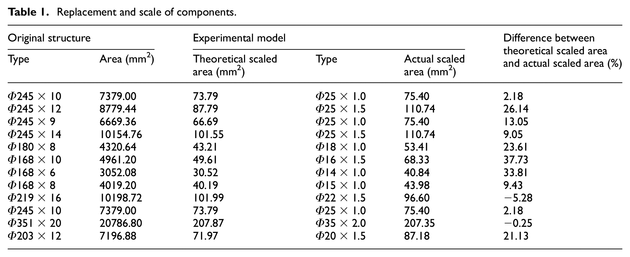
Because the components of the suspended dome are mainly subjected to axial forces, according to the principle of equal axial stress, a 1:10 scale test model of the original suspended dome with a span of 93 m was designed. To verify the test model, a 1:10 scale finite element model and a full-scale finite element model were built, and the analysis results were compared. The loads were applied on the joint of the upper reticulated shell, and the load ratio of the test model to the full-scale building was 1:100. The FEA results showed that the axial stress ratio was 1:1, the joint displacement ratio was 1:10, and the cable tension ratio was 1:100. However, some components are not available on the market at a 1:10 scale, so the test model was not scaled precisely at 1:10. The details of these replaced components are presented in Table 1. The 1:10 scale finite element model was amended according to the real dimensions of the components. The analysis results of the amended 1:10 scale finite element model were close to the 1:10 precisely scaled finite element model. The results of the amended 1:10 scale finite element model were used for comparison with the model test. The stress of the components, the global stability coefficient, and the ultimate bearing capacity coefficient (i.e. the ratio of the ultimate bearing capacity to the design load) of the test model and the actual structure were all approximately equal. The ratios of the joint displacements and cable tensions were 1:10 and 1:100, respectively.

Table 1.

Replacement and scale of components.

Original structure		Experimental model			Difference between theoretical scaled area and actual scaled area (%)
Type	Area (mm²)	Theoretical scaled area (mm²)	Type	Actual scaled area (mm²)
Φ245 × 10	7379.00	73.79	Φ25 × 1.0	75.40	2.18
Φ245 × 12	8779.44	87.79	Φ25 × 1.5	110.74	26.14
Φ245 × 9	6669.36	66.69	Φ25 × 1.0	75.40	13.05
Φ245 × 14	10154.76	101.55	Φ25 × 1.5	110.74	9.05
Φ180 × 8	4320.64	43.21	Φ18 × 1.0	53.41	23.61
Φ168 × 10	4961.20	49.61	Φ16 × 1.5	68.33	37.73
Φ168 × 6	3052.08	30.52	Φ14 × 1.0	40.84	33.81
Φ168 × 8	4019.20	40.19	Φ15 × 1.0	43.98	9.43
Φ219 × 16	10198.72	101.99	Φ22 × 1.5	96.60	−5.28
Φ245 × 10	7379.00	73.79	Φ25 × 1.0	75.40	2.18
Φ351 × 20	20786.80	207.87	Φ35 × 2.0	207.35	−0.25
Φ203 × 12	7196.88	71.97	Φ20 × 1.5	87.18	21.13

Design of components and joints

The test model was scaled according to the engineering design drawings. Because the size of the welded hollow balls was too small to connect components if they were scaled at 1:10, the diameter of the welded hollow ball was enlarged by 1–2 cm to avoid too many components penetrating each other and to ensure welding quality. To simplify the support joint, the reinforced concrete columns located at the support joint were replaced by steel pipe columns with the same lateral stiffness. The bottom of the column was welded on a H200 × 200 × 10 × 12 steel loop beam. The column foot was considered to be rigid because the bending stiffness of the steel beam was sufficiently large. The support of the hollow ball was directly welded onto the top of the steel pipe column because the suspended dome is a self-balancing force system, and the reaction of the support is smaller. As shown in Figure 1, the joint on the top of the strut not only connected the radial and loop components in the upper shell but also connected the strut and radial cables. This configuration may produce a large stress concentration and welding residual stress if all of the components are welded onto the joint ball due to too many weld seams. Therefore, an integral solid cast-steel joint including ball, short pipes, and ear plates was used for the original structure to avoid too many weld seams (Figure 1(a)). The welding position between the components and joints was moved away from the ball to avoid the adverse effects of welding. Because the force of the reduced scale model is smaller than that of the original structure, the welded hollow ball was used to replace the solid cast-steel ball in the test, and the pipes and ear plates were welded onto the ball. The welded hollow ball is sufficiently strong to resist the force without plastic deformation. The joint was not destroyed and showed large deformation during the test, which verified the simplification. A connection device with an adjustable strut from a patent (Zhang et al. 2006) was adopted by the upper joint of the struts in the test model, which could not only release the joint moment of the strut but also apply and adjust the prestress by adjusting the length of the strut. As shown in Figure 2, the top joint of the strut was composed of the following: (1) a hollow ball, (2) the upper fastening of the cardan joint, (3) the lower fastening of the cardan joint, (4) a universal ball with a screw rod, and (5) a steel pipe with an internal thread. The strut could be elongated and shortened by screwing the universal ball with a screw rod to apply or release the force of the strut.

Figure 1.

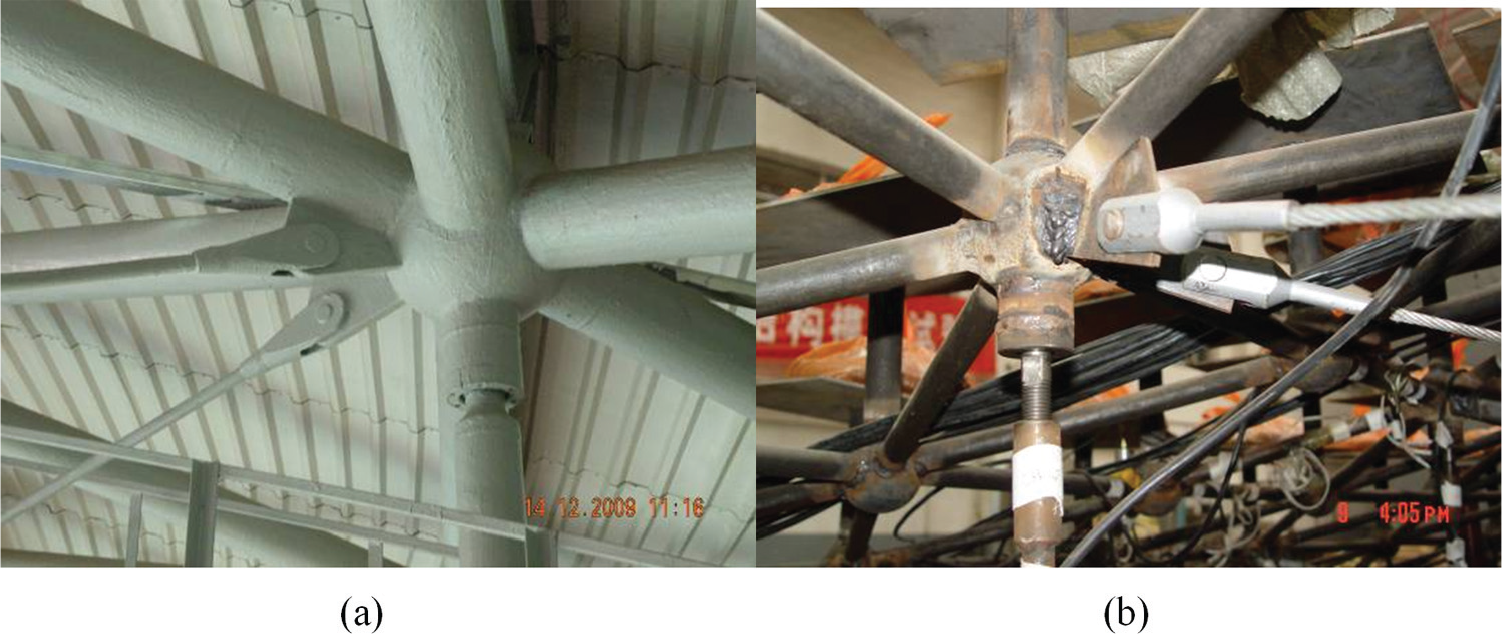
Top joint of strut: (a) joint of original structure and (b) joint of test model.

Figure 2.

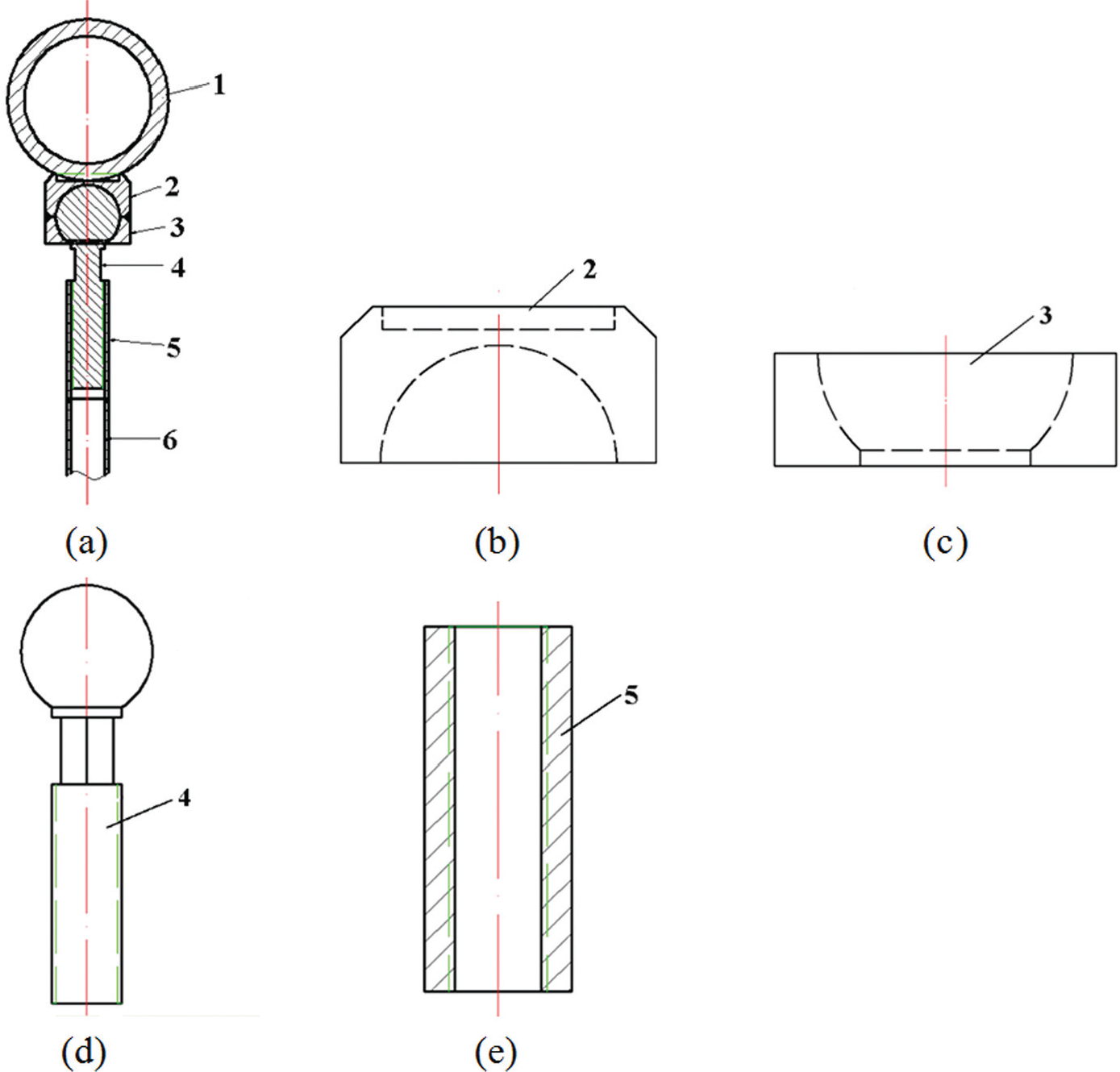
Adjustable top joint of strut: (a) assembly drawing, (b) upper fastening of cardan joint, (c) lower fastening of cardan joint, (d) universal ball with screw rod, and (e) steel pipe with internal thread.

The loop cables were tensioned to apply prestress to the structure. The friction between the cable and the cable–strut joint should be sufficiently small to ensure good sliding performance of the loop cable when the loop cable is tensioned, reducing the prestressing loss in the cables. After tensioning, the loop cable and cable–strut joint were fixed together without sliding under an external load to ensure good global structural stability. As shown in Figure 3, the cable–strut joint of the practical structure is a cast-steel joint. The upper part of the joint was welded to the strut, and one pair of radial steel bars was hinged to the joint by dowels and ear plates. The loop cable passed through the center of the joint; a polytetrafluoroethylene (PTFE) membrane was adhered to the internal surface of the cast-steel joint, and the outside surface of the loop cable was covered by a PTFE membrane, which demonstrated that the friction coefficient at the interface between the loop cable and cast-steel joint was below 0.03. After tensioning, the loop cable was tightly fixed to the cable–strut joint with lower and side bolts.

Figure 3.

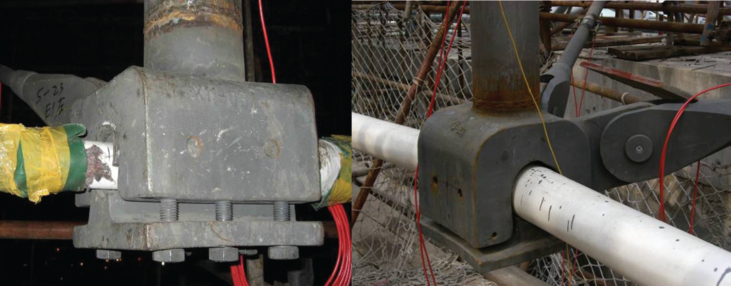
Cable–strut cast-steel joint.

As shown in Figure 4, based on the mechanical properties of the original structure, the cable–strut joint of the test model consisted of a thick steel plate named plate 1 and a thin steel plate named plate 2. There was an arc groove in the middle of plate 1, and the loop cable passed through it. The arc groove was tangent to the loop cable on the planar graph, which ensured good sliding performance between the loop cable and the cable–strut joint. A steel strip was welded onto plate 2, and the plate protruded into the groove to firmly compress the loop cable into the groove after tensioning. The loop cable was wrapped with two layers of PTFE membranes to form three contact interfaces: the interfaces between the loop cable and PTFE membrane, between PTFE membrane and PTFE membrane, and between PTFE membrane and the groove of the cable–strut joint. The friction coefficient between the two PTFE membranes was only 0.03, which caused the two pieces to slide during the tensioning process. The arc groove was tangent to the loop cable, which allowed smooth sliding and significantly reduced the prestressing loss. After tensioning, the PTFE membranes were taken out of the joint, and the steel strip was used to firmly clamp the loop cable into the groove by screwing the three bolts.

Figure 4.

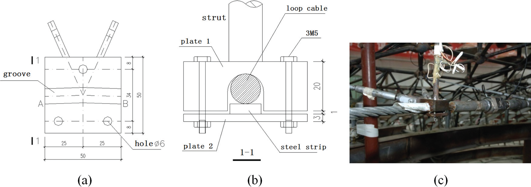
Cable–strut joint used in the model test: (a) plan, (b) profile, and (c) photograph.

The diameter and thickness of the components in the upper shell were generally scaled at 1:10. When the scaled pipe was not available on the market, the components were scaled according to the principle of equal section areas because the forces in the components of the upper reticulated shell were mainly axial forces. However, some components were still not available on the market at 1:10 scale, so the actual replacements of these components are presented in Table 1. As presented in this table, the difference in areas was as high as 37.73% after replacement. However, these were components of the loop truss and struts, which were not the main focus of the experiment. Moreover, these components were designed with a high safety margin and were not damaged before or after the reticulated shell lost global stability. The increased area of these components did not adversely affect the purpose of the test. The difference between the actual scaled area and the precise scaled area for the other components was small after replacement, so they had little effect on the test results.

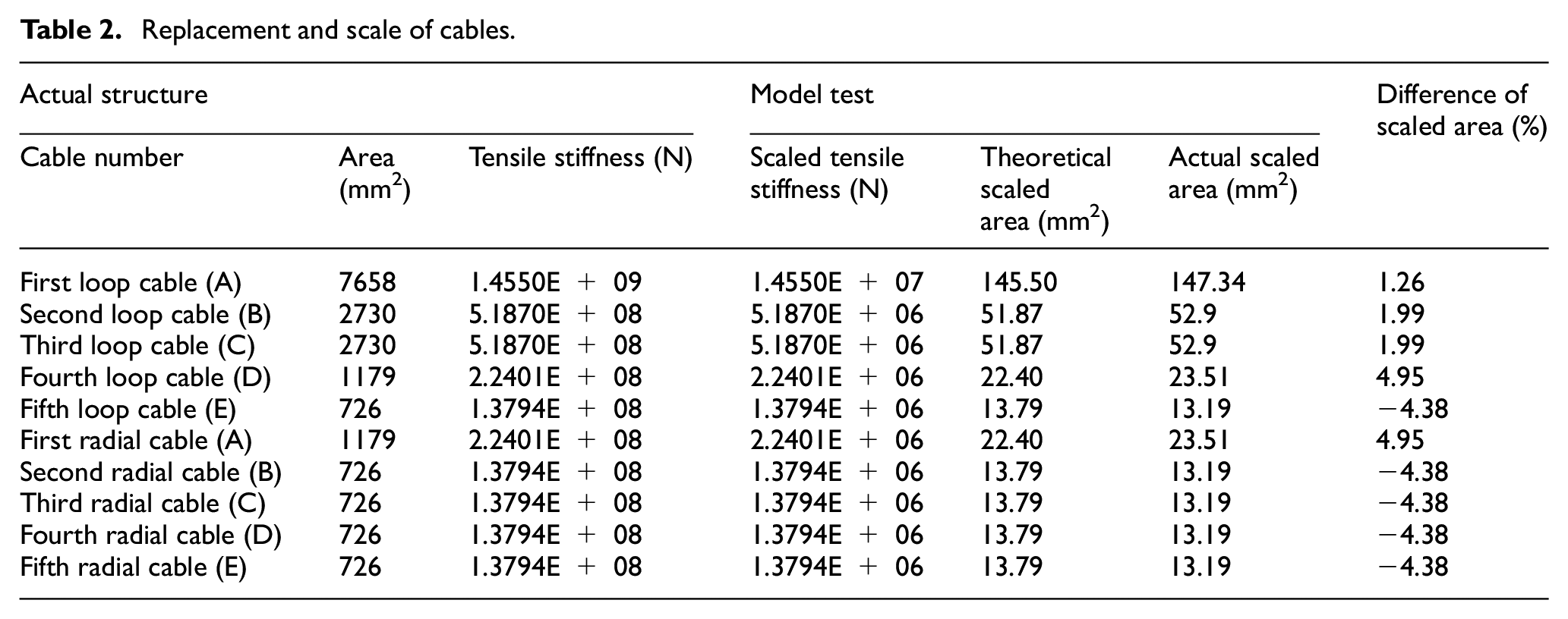
High-strength steel cables were used in the actual structure, but there are no corresponding cables when the area is scaled at 1:100. To ensure that the test model accurately showed the mechanical properties of the actual structure, a steel wire rope was used to replace the steel cable based on the principle that the product of the elastic modulus and area of the cable are equal, that is, the tension stiffness of the cable is equal. The steel wire rope has more dimensions, and its elastic modulus is smaller than that of the high-strength steel cable. The replacement and scale of the cables are presented in Table 2, which shows that the maximum difference between the theoretical scaled area and actual scaled area of the test model is <5% based on the principle of equal tension stiffness.

Table 2.

Replacement and scale of cables.

Actual structure			Model test			Difference of scaled area (%)
Cable number	Area (mm²)	Tensile stiffness (N)	Scaled tensile stiffness (N)	Theoretical scaled area (mm²)	Actual scaled area (mm²)
First loop cable (A)	7658	1.4550E + 09	1.4550E + 07	145.50	147.34	1.26
Second loop cable (B)	2730	5.1870E + 08	5.1870E + 06	51.87	52.9	1.99
Third loop cable (C)	2730	5.1870E + 08	5.1870E + 06	51.87	52.9	1.99
Fourth loop cable (D)	1179	2.2401E + 08	2.2401E + 06	22.40	23.51	4.95
Fifth loop cable (E)	726	1.3794E + 08	1.3794E + 06	13.79	13.19	−4.38
First radial cable (A)	1179	2.2401E + 08	2.2401E + 06	22.40	23.51	4.95
Second radial cable (B)	726	1.3794E + 08	1.3794E + 06	13.79	13.19	−4.38
Third radial cable (C)	726	1.3794E + 08	1.3794E + 06	13.79	13.19	−4.38
Fourth radial cable (D)	726	1.3794E + 08	1.3794E + 06	13.79	13.19	−4.38
Fifth radial cable (E)	726	1.3794E + 08	1.3794E + 06	13.79	13.19	−4.38

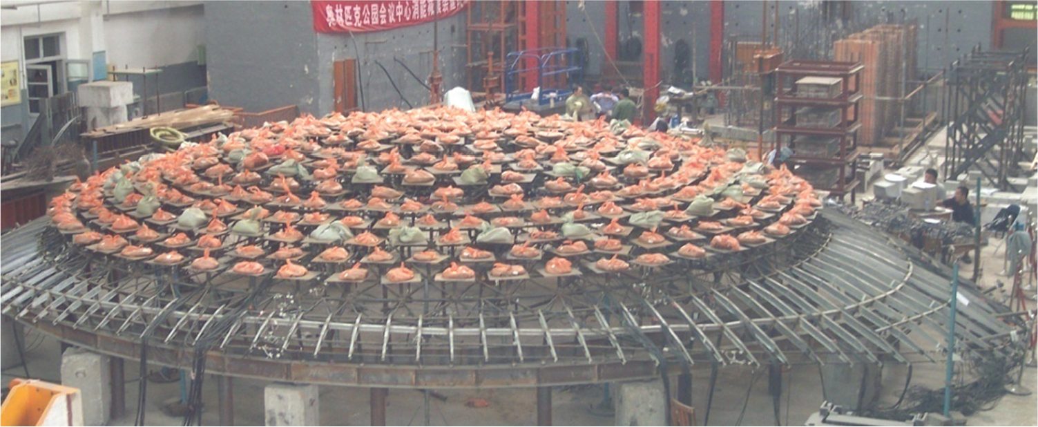
The test model with a span of 9.3 m was built according to the above principle and data. As shown in Figure 9, the top part of the model was a single-layer reticulated shell, which was divided into 13 grids in the radial direction and 56 grids in the hoop direction. There was a circular truss around the single-layer reticulated shell, with web members hinged at both ends resisting axial tension–compression and with chord members fixed at both ends resisting bending and axial forces. The single-layer reticulated shell and circular truss consisted of circular steel tubes; the material was Q345B, and the design tensile strength was 310 MPa. The support system consisted of five-loop cables, radial cables, and struts at the lower part of the model. The axis compressed struts were hinged at both ends and were made of circular steel tubes with Q345B steel. The material of the cables was high-strength cold-drawn zinc-coated wire; the tensile strength was 1870 MPa, and the design strength was 935 MPa.

Load

Because the model was constructed at a scale of 1:10, the length of the component decreased to 0.1 times the original length, the area decreased to 0.01 times the original area, and the weight of the structure decreased to 0.001 times the original weight. When the structure was scaled, assuming that the actual weight of the structure was A, the weight of the scaled model was A/1000. According to the principle of equal stress, the weight of the scaled model should be A/100, so the load was reduced by 9A/1000 when the model was scaled down. Hence, the load that was equal to nine times the weight of the test model was loaded onto the model as an external load to compensate for the reduced 9A/1000 load to reflect the real stress condition of the original structure. A steel plate was placed at each joint in the reticulated shell, without touching each other, to eliminate the mutual influence between each joint load, and some small sandbags were applied on the plate to compensate for the weight. Then, the large sandbags were placed on the plate to load the structure.

Finite element model

The finite element model was built using ANSYS according to the above principles and data with the same dimensions as the test model. The BEAM189 element was used to simulate components in the reticulated shell. The BEAM189 element is suitable for analyzing slender to moderately stubby or thick beam structures. The element is based on the Timoshenko beam theory, which includes shear–deformation effects. The element is a three-dimensional (3D) quadratic three-node beam element. A total of 6 degrees of freedom occur at each node; these include translations in the x, y, and z directions and rotations about the x-, y-, and z-axes. The element is suitable for linear, large rotations and large-strain nonlinear applications. The axial compressive strut and the cable were simulated using the LINK180 element. The LINK180 element simulates the tension-only component to accurately simulate the static character of the cable. The point-to-point contacting element CONTAC178 and the joint coupling technology were used at the lower joint of the strut to consider the friction between the loop cables and cable–strut joint. The CONTA178 represents the contact and sliding between any two nodes of any types of elements. The element has two nodes with 3 degrees of freedom at each node, with translations in the x, y, and z directions. The element is capable of supporting compression in the contact normal direction and Coulomb friction in the tangential direction. The Newton–Raphson iterative method was used for static calculations, considering the geometric nonlinearity and material nonlinearity with the stress stiffening effect.

Tensioning methods and procedures

Tensioning method

Because there are only five loops of cables in the structure, named A, B, C, D, and E, the loop cables were tensioned to apply prestress. There are four tensioning points named A-1, A-2, A-3, and A-4 on the A loop cables. There are four tensioning points named B-1, B-2, B-3, and B-4 on the B loop cables. There are four tensioning points named C-1, C-2, C-3, and C-4 on the C loop cables. There are four tensioning points named D-1, D-2, D-3, and D-4 on the D loop cables. There are two tensioning points named E-1 and E-2 on the E loop cables. The tensioning device of each tensioning point was a turn buckle, and the loop cables were shortened by simultaneously screwing the turn buckles on the same loop cable to apply the prestress. The loop cable was cut near the turn buckle to connect a tension sensor, which could directly read the cable tension, ensuring precise cable tension measurements. The layout of the tensioning points is shown in Figure 5(a), and a picture of a tensioning point is shown in Figure 5(b).

Figure 5.

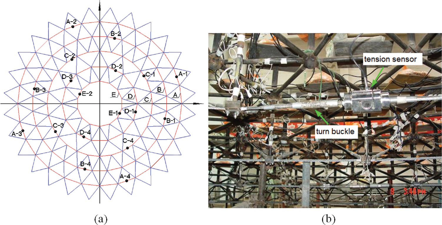
Layout drawing and picture of the tensioning points: (a) Layout drawing and (b) picture of the tensioning points.

Tensioning procedure

Before tensioning, the average friction coefficient of the cable–strut joints for loop cables A, B, C, D, and E was obtained by measuring the test model. While simultaneously tensioning A-1 and A-3, the tensions of A-2 and A-4 were measured, so the force difference between them was caused by the friction at the joint. Therefore, the friction could be derived for the five loops of cables; the friction coefficients of cables A, B, and C were 0.012, and those of cables D and E were 0.006. Before tensioning, all of the measuring devices were set to zero (Figure 6), and a weight load was applied to the structure (Figure 7). Then, different construction schemes were tested on the model. The controlling cable tensions shown in Figure 8 were applied to the tensioning points in sequence.

Figure 6.

Before applying the weight load.

Figure 7.

After applying the weight load.

Figure 8.

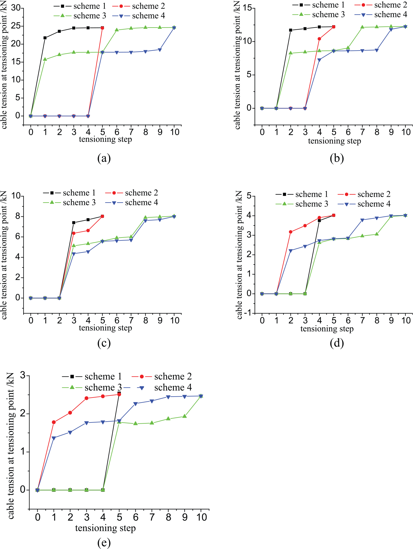
Comparison of the control cable tensions of the loop cables: (a) loop cable A, (b) loop cable B, (c) loop cable C, (d) loop cable D, and (e) loop cable E.

The cable tensions shown in Figure 8 were obtained from construction simulation using the finite element software ANSYS with the following principle and procedure. The initial strain of each tensioning point was calculated based on the principle that the total shortening length of the tensioning points on the same cable loop was equal to the sum of the design values of all of the segments of the same loop cable, and that the design initial strains were uniformly applied on the loop cables in the design stage (Liu et al. 2015). First, the initial strain of each tensioning point was calculated as follows: the design initial strain of a loop cable was multiplied by the total length of the loop cable, divided by the number of tensioning points and then divided by the length of the segment of loop cable where the tensioning point was located. Second, the initial strain of each tensioning point was converted to a negative temperature by dividing it by the linear expansion coefficient. Then, the negative temperatures were applied to the tensioning points according to the tensioning sequence.

Four tensioning schemes were studied in the model. The loop cables were tensioned in the sequence of A-B-C-D-E in scheme 1. First, the four tensioning points A-1, A-2, A-3, and A-4 on loop cable A were tensioned simultaneously, and the tensioning was paused when the cable tensions reached the control values. Rubber hammers were used to knock the loop cables and cable–strut joints, which helped to make the cable tension in the whole loop cable uniform. The cable tension sharply decreased at the first knock and smoothly decreased after several knocks. Then, the tensioning points were tensioned again so that the force at each tensioning point reached the control value again, and the loop cables and cable–strut joints were knocked again. The process was repeated several times until the cable tension stabilized. At that moment, the cable tension of each segment of loop cable was assumed to be the same. Generally, the uniform cable tension obtained after the process was repeated three times. Second, the four tensioning points on cable B were tensioned using the same method. Third, the four tensioning points on cable C were tensioned. Fourth, the four tensioning points on cable D were tensioned. Fifth, the two tensioning points on cable E were tensioned.

The loop cables were tensioned in the sequence E-D-C-B-A in scheme 2 using the same method. In scheme 3, the loop cables were tensioned to 70% of the control cable tension in sequence A-B-C-D-E and then they were tensioned to 100% of the control cable tension in sequence A-B-C-D-E. In scheme 4, the loop cables were tensioned to 70% of the control cable tension in sequence E-D-C-B-A and then they were tensioned to 100% of the control cable tension in sequence E-D-C-B-A.

Figure 8 shows the control cable tension of the tensioning points on each loop cable at each tensioning step of the four tensioning schemes, obtained by FEA. As shown in this figure, schemes 3 and 4 had two tensioning stages, which required more tensioning sequences and higher labor costs than schemes 1 and 2, but the cable tensions changed smoothly. The structure was always in the elastic state during tensioning for each tensioning scheme. Moreover, the friction of the cable–strut joints was small, so the cable tensions of each tensioning scheme were very close at the end of the tensioning process. Because the tensions were applied from the inside to the outside loop cables in schemes 2 and 4, the maximum control cable tensions of the loop cables were larger than that of schemes 1 and 3. In conclusion, the maximum control cable tension in scheme 1 was the smallest, and the tensioning sequence and labor cost were the least, making this the most economical tensioning scheme. Therefore, scheme 1 was the best scheme followed by scheme 2, and these two schemes were selected to be studied in the model test.

Test results

Joint displacement in reticulated shell

As shown in Figure 9, the displacements of only six representative joints, A-3, 1-6, 1-10, 1-15, 43-6, and 43-10, were analyzed because the extra load applied to the structure during the tensioning process was only the weight load, and the structural layout was axisymmetrical.

Figure 9.

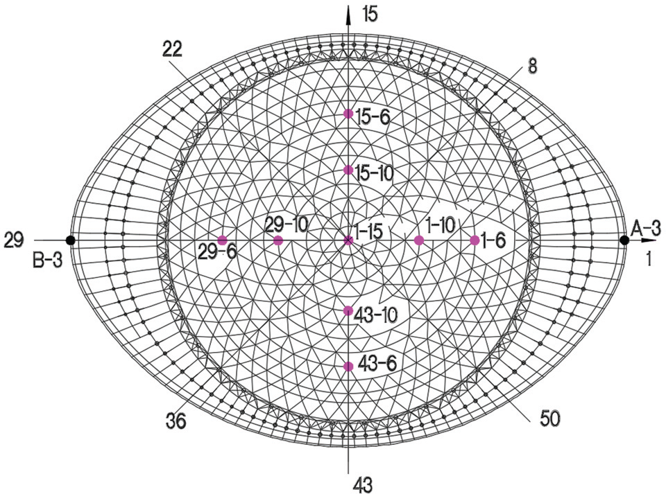
Layout of the vertical displacement measurement points.

Finite element predictions of displacement

Figure 10 shows that finite element predictions of displacement and the experimental vertical displacements of the model were very small during the tensioning process in schemes 1 and 2. The maximum displacement was approximately 1/930 of the span and <10 mm, and geometrical nonlinearity was not obvious. For joints 1-6 and 43-6, the displacements increased in the first two tensioning steps and then decreased in the next three steps in scheme 1, while the displacements decreased in the first three steps and then increased in the next two steps in scheme 2. For joints 1-10 and 43-10, the displacements increased in the first four tensioning steps and then decreased in the last steps in scheme 1, while the displacements decreased in the first step and then increased in the next four steps in scheme 2. For the middle joint 1-15, the displacement increased in the whole tensioning process in scheme 1 but decreased in the first step and then increased in the next four steps in scheme 2. The displacement of joint A-3, which was located on the end of the cantilever beam, was very small for both tensioning schemes, which showed that the cable tensions of the suspended dome had little effect on the surrounding beams. This proved that the suspended dome is a self-balancing force system. In brief, as shown in Figure 10, the vertical displacements of the FEA and test were close, which verified the accuracy of the finite element simulation and showed that the model test and finite element simulation accurately reflected the varying displacements of the joints during the tensioning process. The simulated displacements of the joints of the two tensioning schemes were the same at the end of the tensioning process (tensioning step 5) because the structure was always in the elastic state during tensioning; therefore, the shape of the structure at the end of the tensioning process was the same regardless of the tensioning sequence. However, the situation for the test values was different because of inelasticity and other factors in the tensioning process; therefore, the mechanical characteristics of the structure at the end of tensioning process were dependent on the tensioning sequence. These factors include the nonlinear deformation of the supports, joints, and components; the prestress relaxation of the cables; the friction loss of the cable–strut joints; unequal strut lengths; and initial imperfections and asymmetry in the structural stiffness and force. Measurement error was also a factor. Alls these factors could not be considered in the finite element simulation. The difference between the FEA and experimental displacements indicated that the finite element simulation could not replace the constructional model test for a large-span suspended dome.

Figure 10.

Displacements of the joints: (a) joint A-3, (b) joint 1-6, (c) joint 1-10, (d) joint 1-15, (e) joint 43-6, and (f) joint 43-10.

Axial stresses of components

Because the suspended dome is a self-balancing force system and there was a strong loop truss between the cantilever beams and the suspended dome, although the whole structure was only double-axis symmetric, the mechanical properties of the internal suspended dome and external cantilever beams were relatively independent, and the mechanical properties of the internal suspended dome were approximately centrosymmetric. Therefore, the test and FEA axial stress of loop members 2, 4, 6, 8, and 10 and radial members 15, 17, 19, 21, and 23 were compared. The numbers of the members are shown in Figure 11.

Figure 11.

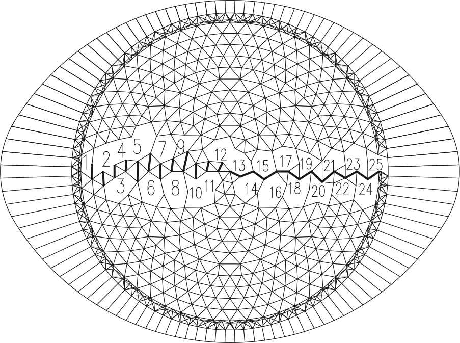
Numbers of the members in the reticulated shell.

Figure 12 shows that the loop members near the loop truss, which were located between loops 1 and 8, had larger stresses during the tensioning process, which were mainly compressive stresses. The finite element predicted values closely match the test values. However, the loop members near the top of the structure, which were located between loops 10 and 13, had smaller stresses during the tensioning process, with a maximum compressive stress of <20 MPa. Although the percentage difference between the finite element predicted and test values was quite large, the absolute difference was smaller. Some radial members had compressive stresses, and some had tensile stresses. The maximum absolute value of the stress during the tensioning process was <30 MPa, which was far below the design strength of the steel of 310 MPa. As shown in Figure 12, during the tensioning process, the maximum stress was in the range of −100 to 35 MPa, which was considerably less than the yield strength of the steel, which was 345 MPa. Therefore, the model was always in the elastic state during the whole tensioning process. The test and finite element predicted values of most members match well.

Figure 12.

Axial stresses of members: (a) member 2, (b) member 4, (c) member 6, (d) member 8, (e) member 10, (f) member 15, (g) member 17, (h) member 19, (i) member 21, and (j) member 23.

Figure 12 shows that the finite element predicted values of the axial stresses of the components in the two schemes were similar but not equal at the end of the tensioning process. As observed in the stress variation curve of the members, the structure was in the elastic state during the whole tensioning process, but the friction of the cable–strut joint was nonlinear and irreversible; therefore, the state of the structure at the end of the tensioning process (i.e. final state) was dependent on the tensioning sequence. However, because the axial stress of the components in the reticulated shell was small and the stress difference between scheme 1 and scheme 2 was small, the final state of the structure was almost not affected by the two schemes, even though they had some effect on the final state in theory. The test values of the stress of the members at the end of the tensioning process in the two schemes were different, and the difference was larger than the finite element predicted values, which indicated that other factors affected the stress in addition to the friction of the cable–strut joint. These factors resulted in the structural performance in the final state associated with the tensioning sequence, including the nonlinear deformation of the supports, joints, and components; the loss of prestressing forces in the cables; the unequal length of the struts; the asymmetry of the structural stiffness and force; and the model fabricating errors. Measurement error was also a factor. All these factors could not be included in the FEA. The difference between the finite element predicted and test values showed that the simulation analysis could not completely replace the model test, although ignoring these factors would not affect the safety of the construction because the structural displacements and stresses were small.

Conclusion

Based on the 1:10 scale finite element model and test model of a large-span suspended dome, four tensioning schemes were studied using finite element simulation. The two better performing tensioning schemes were considered in the model tests. The key conclusions were as follows:

During tensioning, two layers of PTFE membranes were placed between the loop cables and the cable–strut joints, which significantly reduced the friction of the cable–strut joints because slipping was changed from those between steel-and-steel interfaces to those between PTFE membranes. The loop cables can be fixed with the cable–strut joints by bolts and removing or breaking the PTFE membranes after tensioning.

The vertical displacements of the structure were very small during the tensioning, and geometrical nonlinearity was not obvious.

The structure was safe in each tensioning scheme because the maximum stress of the components was small. In scheme 1, in which the loop cables were tensioned from the outside to the inside loop, the maximum tensioning force of the loop cables was minimal, and the loop cable tensions were uniform; therefore, scheme 1 was the best scheme.

The friction of the cable–strut joint was the inelastic factor in the tensioning process that made the cable tension, the force of the components, and the displacement of the joints differ between each scheme at the end of the tensioning process. Therefore, the tensioning process was irreversible. Accurate results for practical engineering can only be obtained considering the inelastic factors in the construction process of the finite element simulation or model test.

In addition to the friction of the cable–strut joints, the nonlinear deformation of the supports, joints, and components; the loss of prestressing forces in the cables; the unequal strut lengths; the asymmetry of the structural stiffness and force; and model fabricating errors were factors that affected the mechanical properties of the structure at the end of the tensioning process. All these factors cannot be considered in the finite element simulation, so the model test was highly necessary. However, these factors did not affect the safety of the structure during tensioning.

Tensioning construction experience of large-span suspended domes is lacking in practical engineering, and finite element simulations of tensioning construction need to be verified by model tests; therefore, a model test is necessary before construction. The model test can precisely predict problems that may occur in construction and ensure the safety and reliability of a large-span suspended dome.

Footnotes

Declaration of Conflicting Interests

The author(s) declared no potential conflicts of interest with respect to the research, authorship, and/or publication of this article.

Funding

The author(s) disclosed receipt of the following financial support for the research, authorship, and/or publication of this article: This work was supported by the National Natural Science Foundation of China (51248009), the Science and Technology Plan of Beijing Municipal Commission of Education (KM201610005012), and the Beijing Natural Science Foundation (8131002).

References

Chen

Yan

Wang

. (2015) Experimental researches of a suspen-dome structure with rolling cable-strut joints. Advanced Steel Construction11(1): 15–38.

Sun

. (2015) New-type suspended structural system design for canopy of Shenzhen North Railway Station. Building Structure4(1): 47–52.

Guo

Dong

(2011) Theoretical and experimental study on tensioning of suspend dome. China Civil Engineering Journal44(2): 65–71.

Guo

Yuan

. (2014) A simple approach for force finding analysis of suspended-domes based on the superposition principle. Advances in Structural Engineering17(11): 1681–1691.

Guo

Wang

Luo

. (2008) Prestressed cable construction of large-span suspended-dome in Ji’nan Olympic Center gymnasium. Construction Technology37(5): 133–135.

Jiang

Wang

Shi

. (2013) Nonlinear buckling analysis of long-span elliptic paraboloid suspended dome structure for Houjie Gymnasium. China Civil Engineering Journal45(2): 21–28.

Jose

AL-G

Ignacio

P-Z

. (2013) Direct simulation of the tensioning process of cable-stayed bridges. Computers & Structures121: 64–75.

Kang

Chen

Lam

H-F

. (2003) Analysis and design of the general and outmost-ring stiffened suspend-dome structures. Engineering Structures25(15): 1685–1695.

Kawaguchi

Abe

Tatemichi

(1999) Design, tests and realization of “suspend dome” system. Journal of the IASS40(131): 179–192.

10.

Kawaguchi

Abe

Hatato

. (1994) Structural tests on the “suspen-dome” system. In:Proceedings of the IASS-ASCE symposium, spatial, lattice and tension structures, conjunction with the ASCE structures Congress XII, 24–28 April 1994, pp. 383–392.

11.

Zhang

Dong

. (2012) Construction sequence simulation of a practical suspen-dome in Jinan Olympic Center. Advanced Steel Construction8(1): 38–53.

12.

Liu

Chen

(2012) Research on effect of sliding between hoop cable and cable-strut joint on behavior of suspen-dome structures. Advanced Steel Construction8(4): 359–365.

13.

Liu

Chen

Zhou

(2012) Research on the process of pre-stressing construction of suspen-dome considering temperature effect. Advanced Steel Construction15(3): 489–493.

14.

Liu

Han

Chen

. (2014) Precision control method for pre-stressing construction of suspen-dome structures. Advanced Steel Construction10(4): 404–425.

15.

Liu

Zhang

(2015) Cable tension preslack method construction simulation and engineering application for a prestressed suspended dome. Advances in Materials Science and Engineering 2015: 651041-1–651041-17.

16.

Luo

Guo

Feng

. (2009) Stability research on elliptic paraboloid suspen-dome of Changzhou Municipal Gymnasium. Journal of Building Structures45(3): 6–9.

17.

Meng

. (2011) Structural design of suspend-dome structure of Pingshan Basketball Gymnasium for Universidad 2011 Shenzhen. Building Structure41(4): 24–28.

18.

Nie

Fan

Zhi

(2013) Test on the suspended dome structure and joints of Dalian Gymnasium. Advances in Structural Engineering16(3): 467–485.

19.

Nie

Zhi

Fan

. (2012) Study of the tension formation and static test of a suspendome for Dalian Gymnasium. China Civil Engineering Journal45(2): 1–10.

20.

Sun

. (2015) Pre-stressing simulation and experimental study of new type suspended roof in platform canopy of Shenzhen North Railway Station. Building Structure45(1): 53–57.

21.

Wang

Zhang

Wang

. (2009) Structure design and research of steel large span suspended dome of the gymnasium in Sanya Sports Centre. Building Structure39(10): 67–72.

22.

Wang

Guo

Luo

(2008) Emulation analysis of hoop cable tension construction of large span cable-supported single-layer elliptical lattice shells. Construction Technology36(6): 58–60.

23.

Wang

Chen

. (2015) Suspend-dome structure design and analysis for steel roof of bicycle gymnasium in Tianjin Sports Center. Building Structure45(5): 6–9.

24.

Wang

Qin

. (2006) Experiment study on two type of cable arrangements of the double ellipse suspend dome. Industrial Construction 36(Suppl.): 477–480.

25.

Wang

Zhang

. (2012) Research on prestress construction technology of Yubei Gymnasium in Chongqing city. Spatial Structures18(3): 60–67.

26.

Ding

. (2008) Structural analysis and design of suspendome roof of gymnasium of Lianyungang. Building Structure38(9): 32–36.

27.

Yan

. (2015) Analysis and design of suspendome structure roof of Qinyang Gymnasium. Building Structure45(3): 6–9.

28.

Zhang

Liu

(2007) Suspen-dome optimal design of Olympic badminton stadium based on integral stability. Building Structure37(21): 1–5.

29.

Zhang

Liu

(2007a) Optimization and determination of prestressed suspend-dome system of the badminton gymnasium for 2008 Olympic Games. Journal of Building Structures28(6): 1–9.

30.

Zhang

Huang

Zhang

(2007b) All course analysis of suspendome construction. Industrial Construction37(4): 55–59.

31.

Zhang

Liu

(2007c) Stability analysis of suspend-dome of badminton gymnasium for 2008 Olympic Games. Industrial Construction37(1): 8–11.

32.

Zhang

Liu

Wang

. (2007) A Kind of Connecting Device of Joint with Adjustable Strut for Prestressing Steel Structure. Patent: CN 200620113789.2.

33.

Zhang

Liu

Wang

. (2007d) Static experimental study on the model of the suspend-dome of the badminton gymnasium for 2008 Olympic Games. Journal of Building Structures28(6): 58–67.

34.

Zhang

Qin

. (2007e) Simulating analysis of prestressing construction process of the suspend-dome of the badminton gymnasium for 2008 Olympic Games. Journal of Building Structures28(6): 31–38.

35.

Zhang

Chen

. (2010) Structural prestress monitoring of Lianyungang gymnasium suspen-dome. Journal of Vibration, Measurement & Diagnosis30(2): 181–183.

36.

Zhang

Dong

. (2008) Structural design of the suspen-dome for the gymnasium of Jinan Olympic Sports Center. Spatial Structures14(4): 8–13.