




Abstract
Due to the complexity involved and limited study on the topic, the equivalent static method, adopted in the current codes for structural design of bridges under ship collisions, does not take into account the dynamic amplification effect correctly. In this article, impact factor method is proposed to estimate the response of bridge’s piers and foundations, as a better alternative of the equivalent static method. Through refined numerical simulations of ship-rigid wall collisions for nine typical ships under various impact velocities, 81 impact force time-histories are obtained. The period-dependent impact factor is defined, and empirical function of it is proposed and parameters in the empirical function are determined by the 81 sample impact force time-histories. Finally, both impact factor method and dynamic time-history method are used to estimate the responses of piers and foundations of two example bridges, and the precision of impact factor method is discussed.
Keywords
Introduction
Vessel–bridge collision demand analysis aims at studying the response of bridge structure under vessel collision. Nowadays, the equivalent static load method, the finite element numerical simulation method, and the simplified dynamic analysis method are mostly used for demand analysis of vessel–bridge collision.
The equivalent static method is employed in most codes and specifications (Knott and Damgaard, 1990; Knott, 2010; Vrouwenvelder, 1998) for vessel collision design of bridges. However, the problem is that code formulas may provide impact force estimations that differ from one another (Wang et al., 2006). In addition, the dynamic characteristics of vessel–bridge collision are ignored.
For more than 10 years, the finite element model (FEM) has been widely used in numerical simulations of ship–bridge collisions (Consolazio and Cowan, 2003, 2005; Ocakli et al., 2004; Wang and Chen, 2007, 2009), and validation verifications of the FEM have been conducted by various academic organizations (Association for Structural Improvement of the Shipbuilding Industry (ASIS) 1993; International Ship and Offshore Structures Committee (ISSC), 2003). Although almost all dynamic characteristics can be considered, higher requirements to the researchers and heavy calculation are required for the finite element numerical simulation method, which is not practical for engineering applications.
Therefore, efforts have been paid to develop the simplified methods to estimate the impact response of bridge under vessel collisions. For example, impact response spectrum analysis method for barge-bridge collision has been proposed (Cowan, 2007; Fan and Yuan, 2012; Wang and Yu, 2014). However, the time duration of vessel–bridge collision is far shorter than the duration of seismic ground motions. Therefore, the concept of seismic response spectra and corresponding modal combination methods might not be suitable to apply to the impact response estimation for vessel–bridge collisions.
In this article, an impact factor method (IFM) for design of bridge piers and foundations under vessel collisions is developed. The period-dependent impact factor (PDIF) is developed based on numerical simulations of vessel–bridge collisions. The response of bridge piers and foundations may be estimated by static response multiplied by the impact factor. Finally, the precision of IFM is verified by two example bridges.
Impact force time-history of ship–bridge collision
In this article, nine typical ships are chosen with deadweight tonnage (DWT) ranging from 500 to 50,000, as listed in Table 1, and the configurations of the ships are illustrated in Figure 1.
Feature data of example ships.

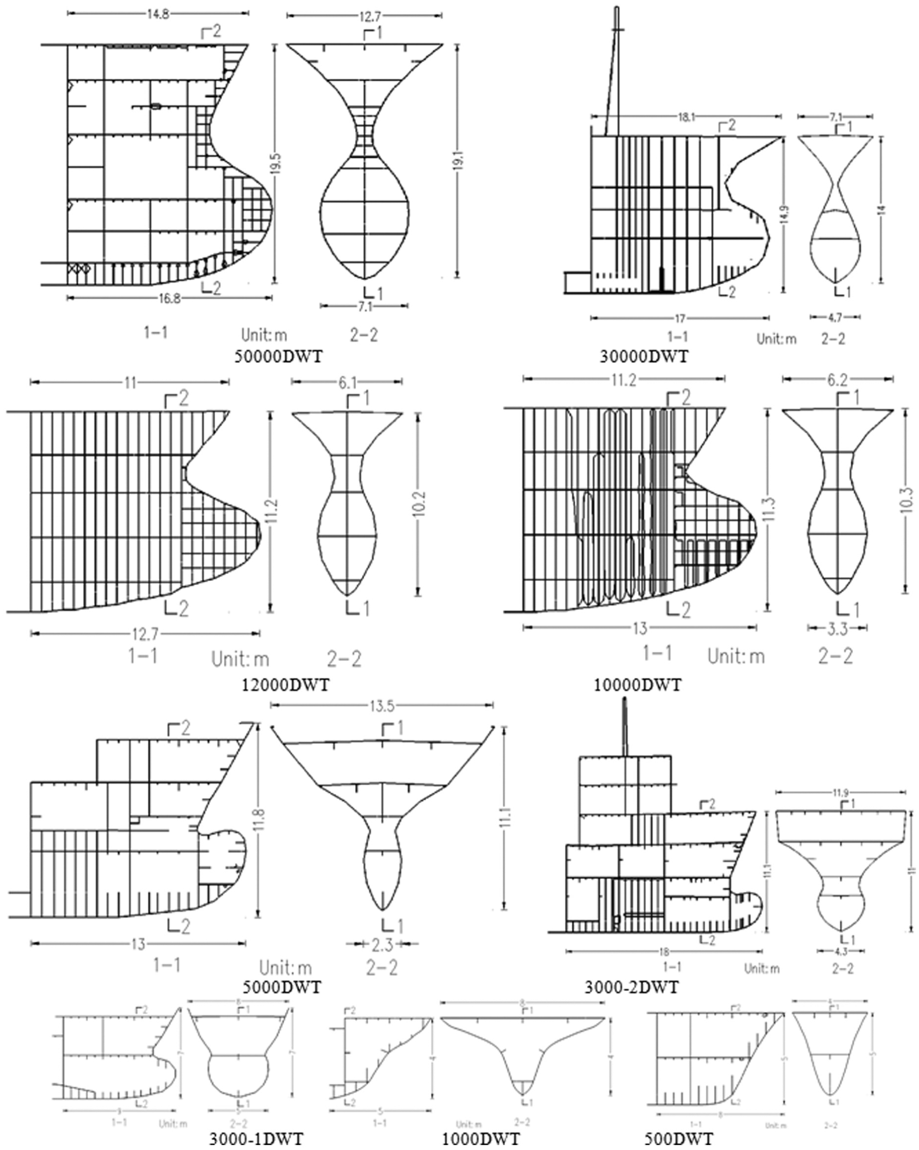
Configurations of typical ships.
To obtain the impact force time-history of ship–bridge collision, the simplified computational model for ship-rigid wall collisions as shown in Figure 2 is used instead of the complex ship–bridge components collision cases. The FEMs of typical ships by software LS-DYNA are illustrated in Figure 3 for the ship-rigid wall head-on collisions. The reliability of the numerical simulation has been well stated in the literatures (Consolazio and Cowan, 2003, 2005; Liu and Gu, 2003; Wang et al., 2013; Wang and Gu, 2001; Yuan and Harik, 2009).
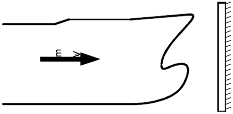
Ship-rigid wall head-on collision model.
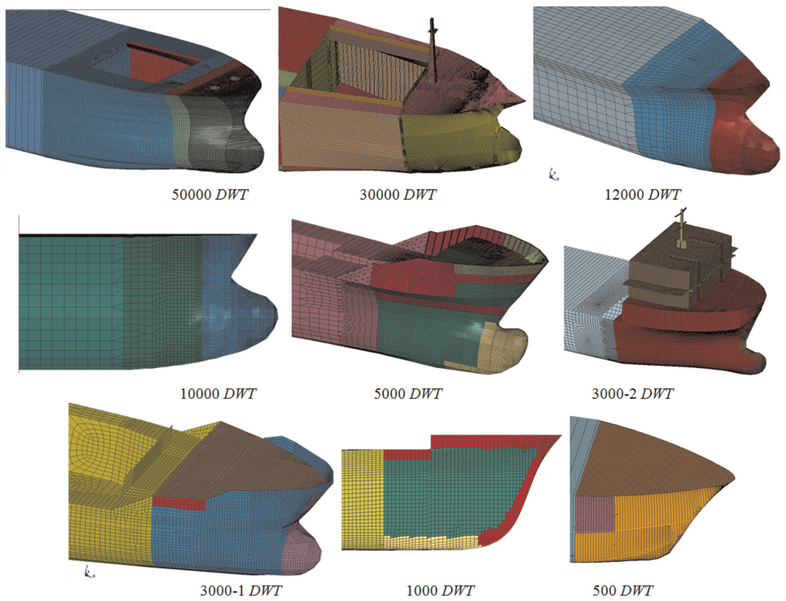
Finite element models of ship bows.
The collision velocity is taken as 1.0, 1.5, 2.0, 2.5, 3.0, 3.5 4.0, 4.5, and 5.0 m/s. The numerical computations for the ship-rigid wall head-on collisions associated with nine ships and nine velocities are finished, and totally 81 samples of impact force time-histories are obtained. Example curves of the impact force time-history are illustrated in Figure 4.
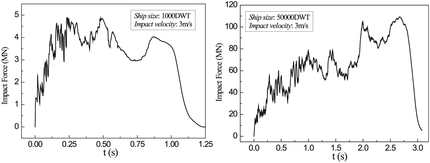
Example curves of the impact force time-history.
Period-dependent impact factor
Definition of PDIF
And the dynamic equation of motion of a single degree-of-freedom (SDOF) system with unity mass can be expressed as follows

where ξ is the damping ratio; ω is the circle frequency of SDOF; δ(t) is the time varying displacement; and
The maximum dynamic response of SDOF system under the impact force time-history can be determined through the combined use of static response calculation and a dynamic magnification factor which is defined as PDIF

where
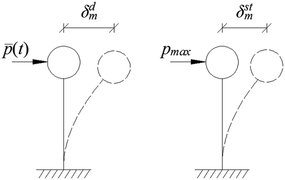
Responses of SDOF system.
The solution of equation (1) can be expressed by Duhamel integration as follows
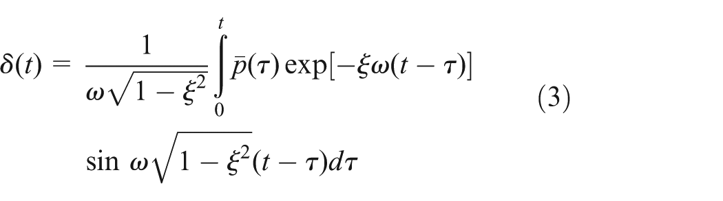
Following the definition of PDIF (equation (2)) and the solution of
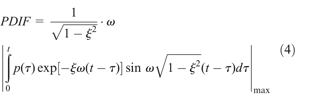
where |.|max means absolute maximum value.
Samples of PDIF
By solving equation (4) excited by impact force time-histories given in section “Impact force time-history of ship–bridge collision,” the 81 PDIFs are obtained, and two examples are shown in Figure 6 with λ = td/T, where td is the equivalent impact duration and T is the free vibration period of SDOF.
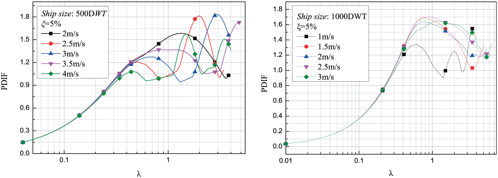
Example curves of the result of PDIF.
It is reasonable to use td/T as the horizontal axis for short-time impact action (Chopra, 2012). To define td, it is assumed that the impact force time-history might be equivalent to a half-sine function, as shown in Figure 7. According to the equal-impulse principle, td is the equivalent duration of the sample impact force time-history and is defined as follows


where I0 is the impulse corresponding to the sample impact force time-history.
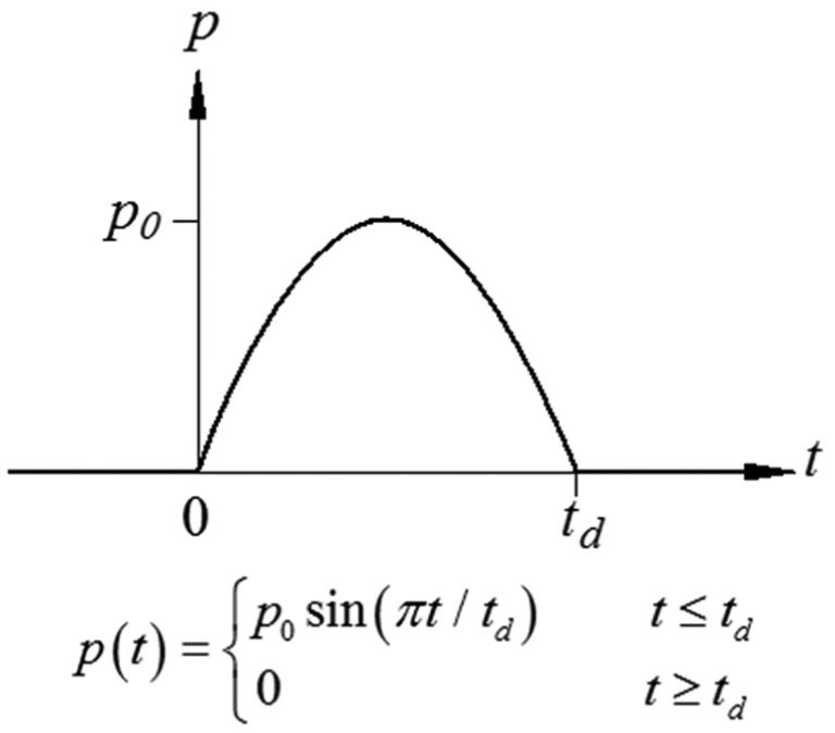
Equivalent duration definition, td.
The 81 samples of PDIF are shown in Figure 8 for damping ratio, ξ, of 0.05. One can observe from Figure 8 that the PDIF is related to the ship’s size, impact velocity, and λ. It is observed that the PDIF might be divided into three phases, the first phase increases significantly with λ, the second phase nearly maintains a constant in average meaning and the third phase approaches to 1.0 as λ increases.
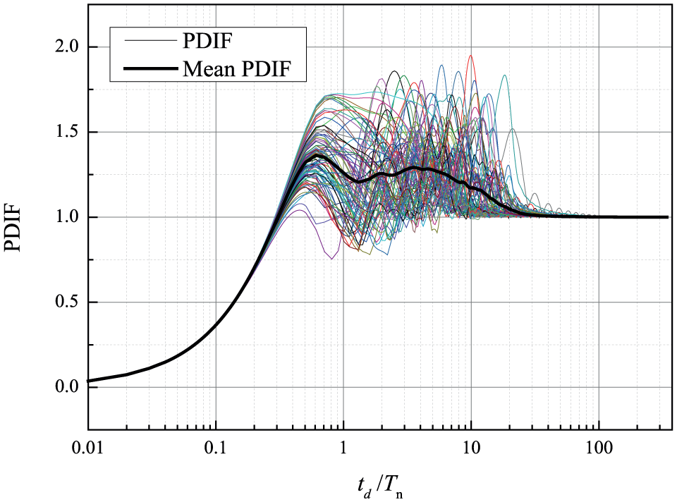
Samples of PDIF.
PDIF for designs
Empirical expression of PDIF
For bridge’s design under ship collisions, an empirical expression of PDIF with statistical meaning is necessary. Generally, contributions of very higher modes (say, natural frequencies higher than 6 Hz) to important structural responses are insignificant as shown in Figure 14 later, that is, rough values for the third phase might not lead to large errors to the structural responses. Therefore, it is proposed that the design value of PDIF (named as DPDIF) takes the following expression

where k and λ1 are the statistical coefficients. The graph of the function corresponding to equation (7) is shown in Figure 9.
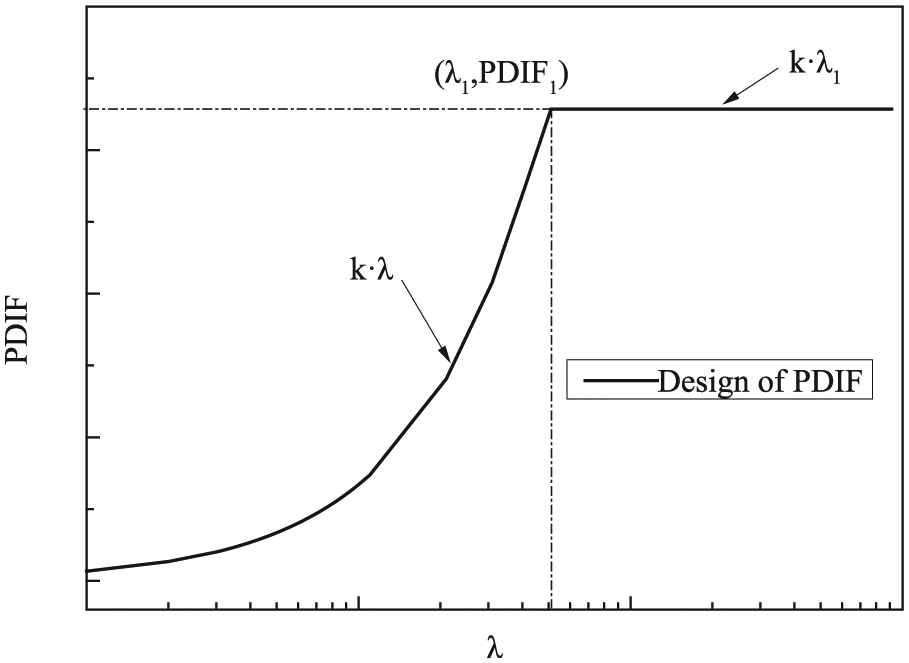
Shape of the DPDIF.
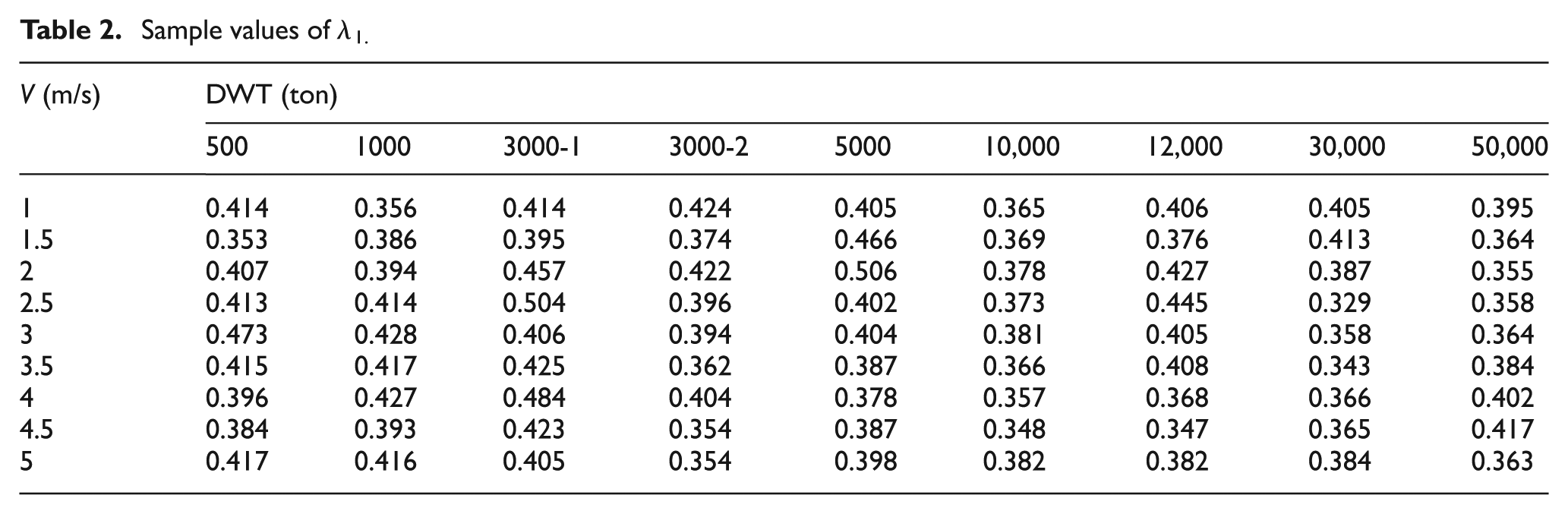
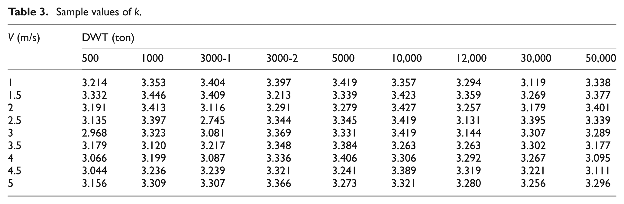
By least square fitting based on the 81 samples of PDIF, the sample values of k and λ1 are obtained as listed in Tables 2 and 3. According to Tables 2 and 3, only small dispersion of k and λ1 is observed, that is, the standard deviations of k and λ1 are small. Therefore, it is proposed that the mean values of k and λ1 may be used in designs, with k = 3.273 and λ1 = 0.396. Two examples of the DPDIF and the corresponding sample PDIF are shown in Figure 10.
Sample values of λ1.
Sample values of k.
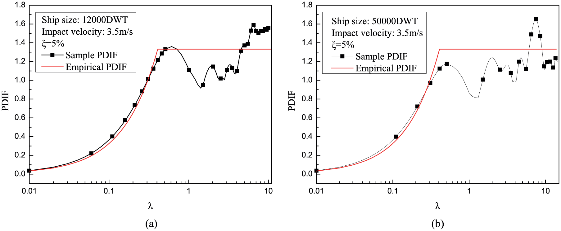
Examples for DPDIF samples: (a) 12,000 DWT and (b) 50,000 DWT.
Empirical expression of pmax and td
According to equations (2) and (7), to use empirical PDIF in designs, it is necessary to know the empirical formulations of pmax and td. For the 81 samples of impact force time-histories, the samples of pmax and td are listed in Tables 4 and 5, respectively.
Sample values of pmax (MN).

Sample values of td (s).
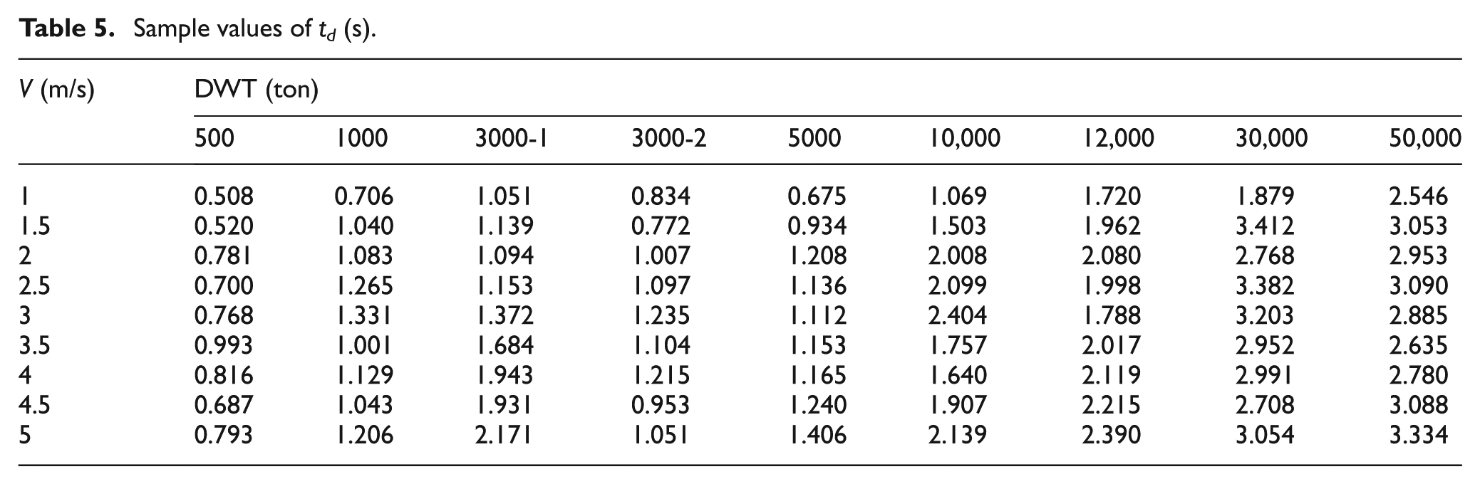
It is observed from Tables 4 and 5 that the pmax and td are related to the loaded displacement of ship and the impact velocity. The following functions are proved to be more accurate when compared with other empirical expressions


where pmax is in MN, td is in second, M is the ship loaded displacement (ton), V is the impact velocity (m/s), and values of α1, α2, β1, β2, and γ1, γ2 are statistical factors.
By statistical analysis of the data of Tables 4 and 5, we obtain that α1 = 0.0224, β1 = 0.8726 and γ1 = 0.6782, and α2 = 0.0578, β2 = 0.3393 and γ2 = 0.1505, respectively. Indexes, ε1 and ε2, are introduced to evaluate the precision of equations (8) and (9), as defined follows,

where

Relative error of empirical values of pmax and td: (a) ε1 and (b) ε2.
IFM for design of bridge piers and foundations
The dynamic equation with multi-degree of freedom for bridge under impact of ships may be expressed as follows

where
Follow the general theory of dynamics of structures (Chopra, 2012), taking linear transform

where

where qj is the generalized coordinates of mode j, ξj is the modal damping ratio of mode j, ωj is the circle frequency of mode j,

where δj is the time varying displacement of SDOF system under
For any response, r(t) of bridge structure may be expressed as (Chopra, 2012) follows

where rj(t) is the response of mode j and
Assuming that the peak values,
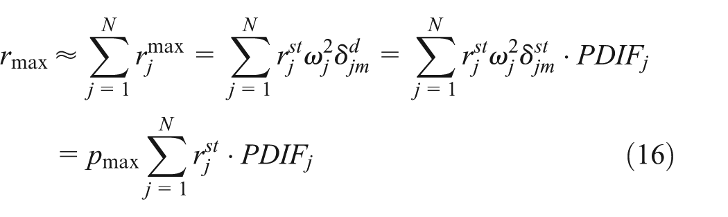
in which
Based on equation (16), it is further assumed that PDIFs for all modes are equal to the value of PDIFmax corresponding to the mode which contributes greatest to the total response, thus
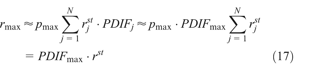
where rst is obtained by solving the following static equation

Equation (17) is called the IFM. To determine PDIFmax, mode contribution ratio, βj, is introduced to evaluate the response contribution of mode j

where
However, it is not practical to use βj to determine PDIFmax, because time-history analysis is necessary to get the modal response. Thus, another index,

where |Γ|max = max{|Γ1|, |Γ2|, … ,|Γ N |}.
The validity of the assumptions adopted by SUM and IFM will be stated in section “Examples and discussions” through two example bridges and the precision of SUM and IFM will be discussed.
Examples and discussions
Basic information and analysis models of the example bridges
To demonstrate the precision of SUM and IFM, both IFM and dynamic time-history method are employed to estimate the responses of two example bridges, one is a cable-stayed bridge and the other one is a continuous girder bridge. Such bridge types are quite common for bridges crossing navigation channels.
The cable-stayed bridge is of a length of 1430 m with five spans and two towers. Its span arrangement is 110 m + 240 m + 730 m + 240 m + 110 m. The group pile foundation of the pylon consists of 60 piles of 104 m long with variable diameters of 2.5 and 3.2 m. The group pile foundations of the auxiliary piers and the side piers are designed with 18 and 12 piles, respectively. The concrete grade of the foundation is C30.
The continuous girder bridge includes five spans each measuring 55 m. The group pile foundation of the pier consists of seven inclined piles with diameter of 1.6 m (Figure 12).
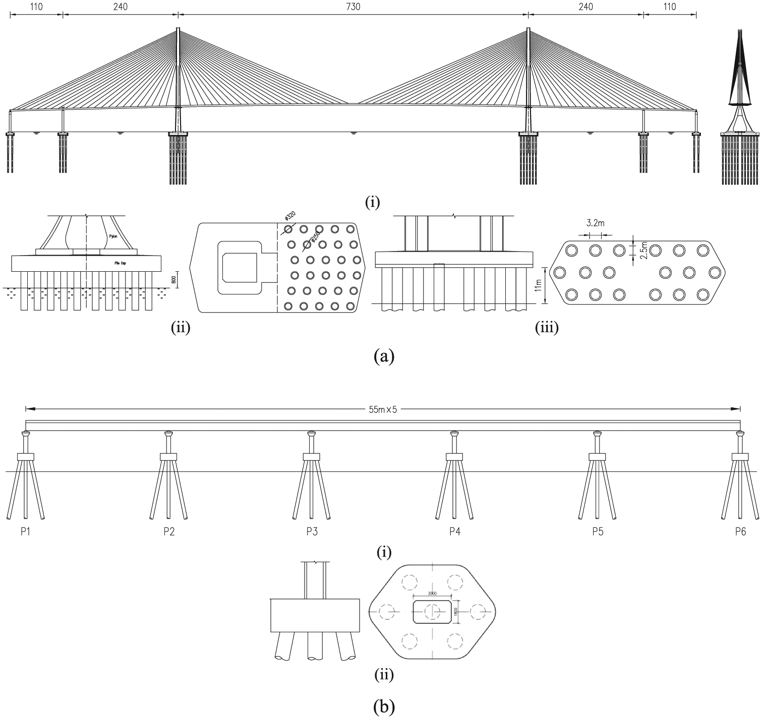
Configurations of the example bridges. (a) The cable-stayed bridge: (i) overall elevation, (ii) tower and group pile foundation, and (iii) auxiliary pier and group pile foundation. (b) The continuous girder bridge: (i) overall elevation and (ii) pier and group pile foundation.
The bridge components are modeled with beam element. In order to accounting for the soil–pile interaction of the cable-stayed bridge, discrete springs are used to simulate the soil. The piles of the continuous girder bridge were fixed at the position of the riverbed. FEMs for static and dynamic analysis are illustrated in Figure 13.
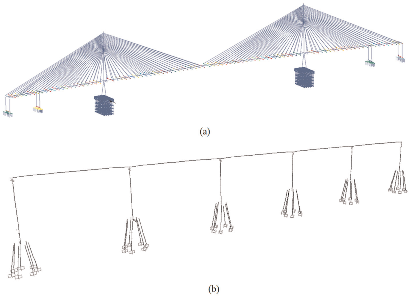
Finite element models of the example bridges: (a) the cable-stayed bridge and (b) the continuous girder bridge.
Impact loads and analysis cases
To demonstrate the precision of SUM and IFM, five kinds of response analysis of example bridges are performed as listed in Table 6.
Analysis cases.
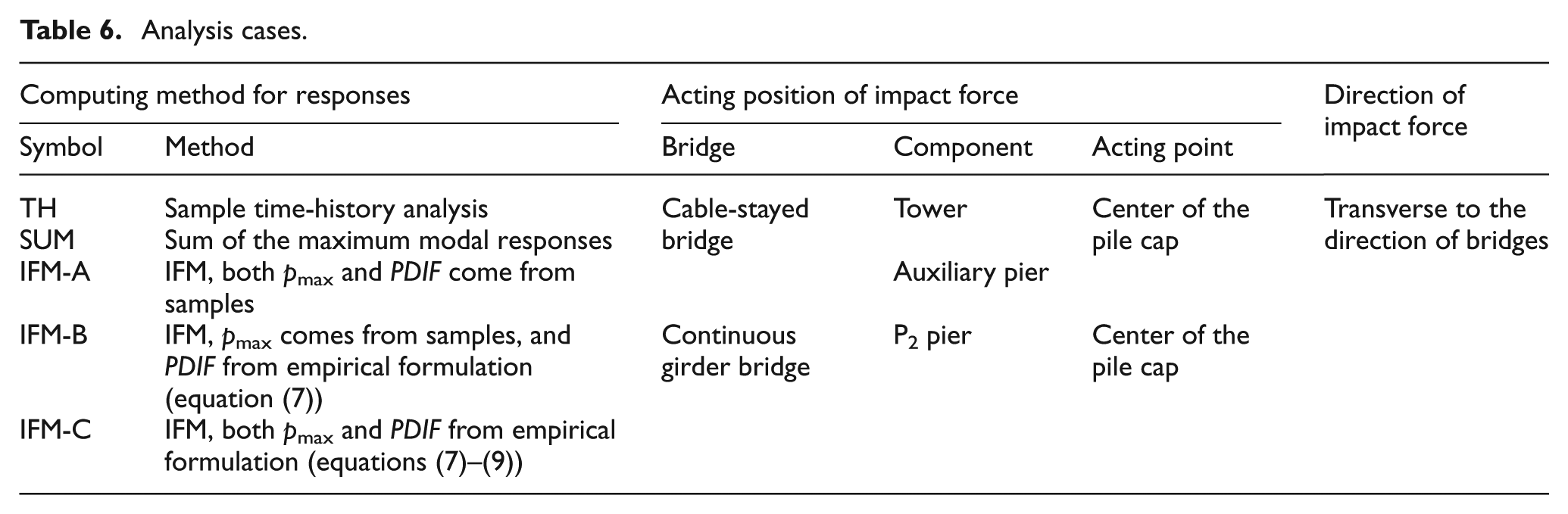
The sample impact force time histories come from ships of 50,000 DWT and 5000 DWT with impact velocity of 3 m/s for the cable-stayed bridge, respectively; 5000 DWT with 3 m/s, 1000 DWT with 4 m/s, and 500 DWT with 2 m/s for the continuous girder bridge, respectively.
Precision of IFM
By conducting calculations in Table 6, βj of the case TH for the two example bridges is shown in Figure 14. f in Figure 14 is the modal natural frequency in Hertz. The symbol meanings of CPCT/5000, CPCAP/5000, and CPCP2/1000 will be explained later in Tables 7 and 8.
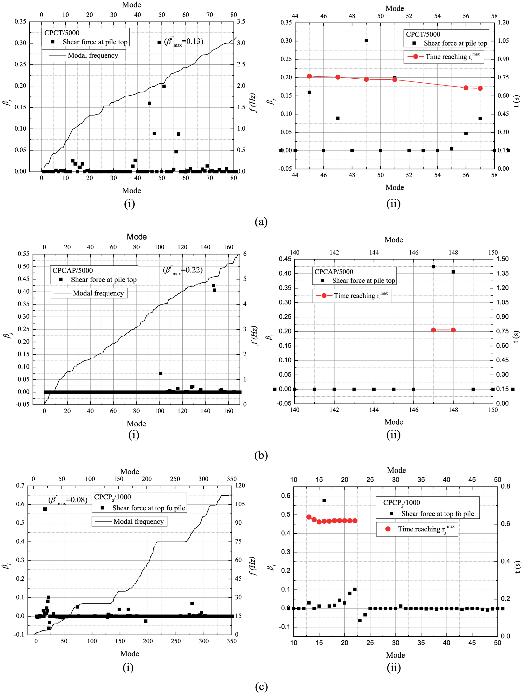
Modal response features. (a) Tower of the cable-stayed bridge: (i) βj and modal frequency and (ii) βj and time reaching
Precision of SUM and IFM impacted at center of pile cap of the cable-stayed bridge.
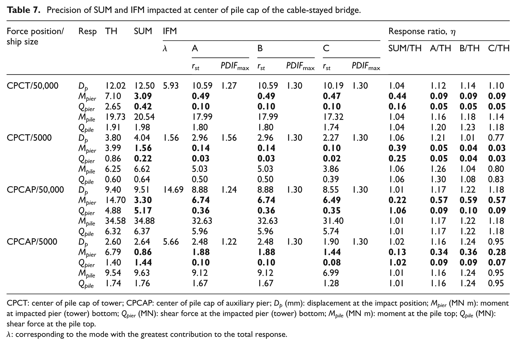
CPCT: center of pile cap of tower; CPCAP: center of pile cap of auxiliary pier; Dp (mm): displacement at the impact position; Mpier (MN m): moment at impacted pier (tower) bottom; Qpier (MN): shear force at the impacted pier (tower) bottom; Mpile (MN m): moment at the pile top; Qpile (MN): shear force at the pile top.
λ: corresponding to the mode with the greatest contribution to the total response.
Precision of SUM and IFM impacted at center of pile cap of continuous girder bridge.
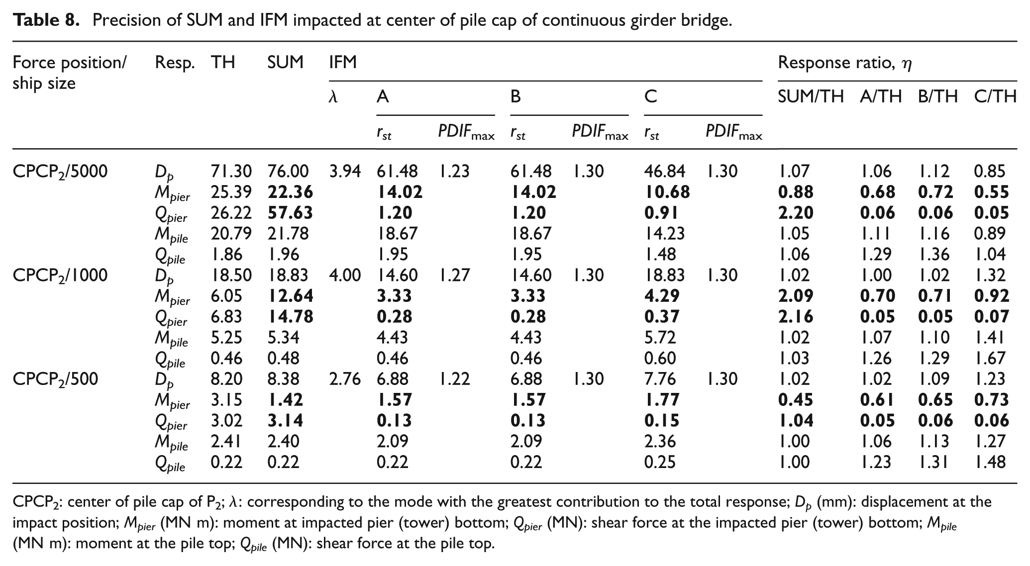
CPCP2: center of pile cap of P2; λ: corresponding to the mode with the greatest contribution to the total response; Dp (mm): displacement at the impact position; Mpier (MN m): moment at impacted pier (tower) bottom; Qpier (MN): shear force at the impacted pier (tower) bottom; Mpile (MN m): moment at the pile top; Qpile (MN): shear force at the pile top.
Figure 14 shows the following valuable information:
Only a few modes contribute the most part to the total response, called “important modes” and the left modes contribute a small part to the total response;
βj of the “important modes” have the same sign. Then, according to equation (19),
The modal natural frequencies, f (in Hz), of the “important modes” are very closely spaced. In other words, these modes reach the peak response nearly at the same time and PDIFs of the “important modes” are nearly the same.
The mode with the greatest contribution to the total response determined by
To evaluate the precision of SUM and IFM, define the following ratio

where rSUM and rIFM represent the response obtained by SUM and IFM, respectively, and rTH represents the peak response by time-history analysis. The responses of the two example bridges are listed in Tables 7 and 8, in which the symbol meanings are explained in Table 6.
From Tables 7 and 8, some observations can be reached as follows:
Both SUM and IFM are suitable to calculate the responses of bridge components below the impact position, but are not suitable for responses above the impact position. Specifically, for responses below the impact position, the relative error does not exceed 7% for SUM and is mostly in the range of ±20% for IFM. However, for responses above the impact position, the precision of SUM and IFM is poor, which is highlighted in bold. For instance, η of Mpier of A/TH for CPCT/50,000 is 0.09 and for CPCP2/5000 is 0.68;
Compared with IFM, SUM could get more accurate results for responses below the impact position. SUM assumes that the peak values of modal response rj(t), j = 1, 2, … , N, have the same sign and occur at the same time. According to Figure 14, for “important modes,” the assumptions of SUM are quite reasonable and lead to minor error (not more than 7% for the two example bridges); IFM assumes that PDIFs for all modes equal to PDIFmax, which is a relatively stronger assumption than SUM. For the two example bridges, the errors of IFM are smaller than ±20% in general, and slightly larger than SUM;
By Comparing the IFM precision of responses below the impact position through the methods of A, B and C, it reveals that neither of these is constantly better than the other two. For instance, η of Dp for CPCT/50,000, CPCT/5000, and CPCP2/5000 gets the best precision by methods C, B, and A, respectively. In fact, the errors of IFM come from two aspects, one is the assumptions of IFM, as stated in section “Impact factor method for design of bridge piers and foundations”; and the other is the statistical errors of equations (7)–(9) for DPDIF, pmax and td. Therefore, it does not mean that the precision of IFM using DPDIF, pmax, and td is always poorer than that using sample values;
Figure 15 shows that the modes with significant contributions to Dp are the same as that to Mpile and Qpile, and even βj of these modes are nearly equal for Dp, Mpile, and Qpile, respectively. Therefore, for different responses of components below the impact position, values of PDIFmax could be taken equal when using sample values for PDIF, as shown in Tables 7 and 8;
According to Table 2, λ1 < 0.5. From Figure 15, it shows that λ of all the modes with non-zero contributions to the total response are larger than λ1. Therefore, DPDIF takes its value at the second part in Figure 9, that is, DPDIF takes a constant value in statistical sense. In this case, IFM is identical to SUM. Furthermore, larger λ might be expected for bridges with smaller spans, and therefore, IFM is suggested to estimate the responses of bridge components below the impact position for design under ship impact.
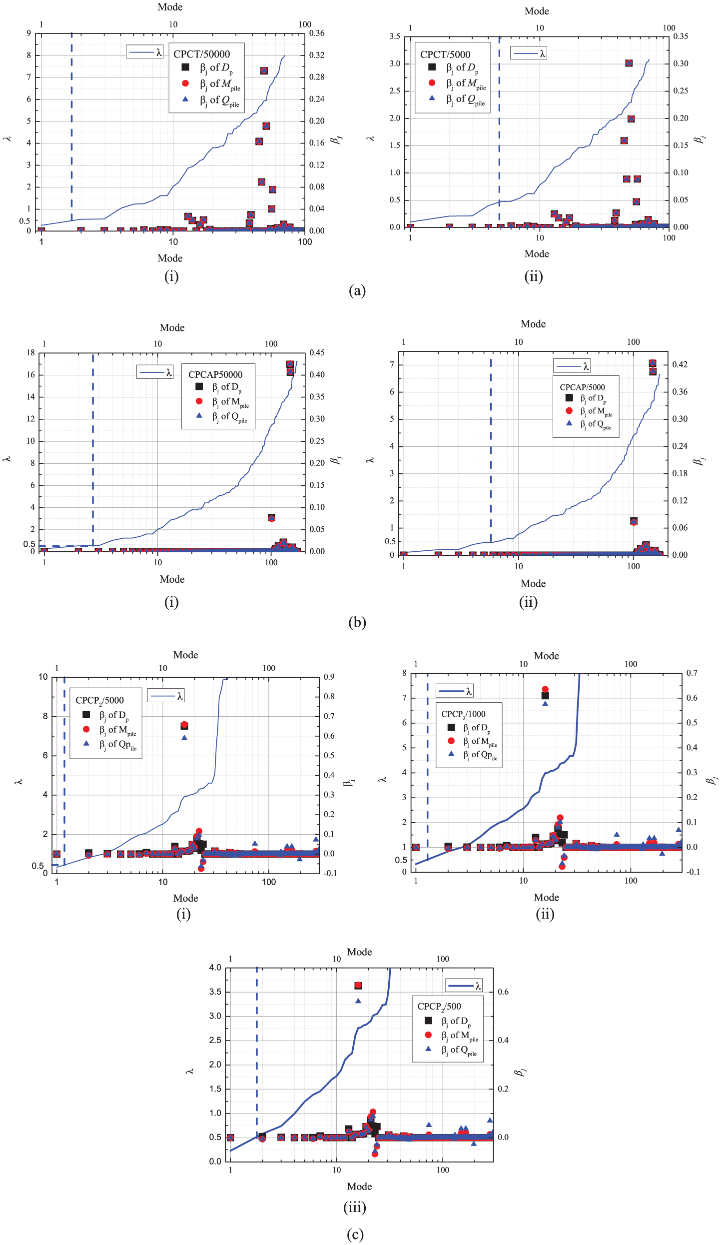
λ for considered modes. (a) Tower of the cable-stayed bridge: (i) CPCT/50,000 and (ii) CPCT/5000. (b) Auxiliary pier of the cable-stayed bridge: (i) CPCAP/50,000 and (ii) CPCAP/5000. (c) P2 of the continuous girder bridge: (i) CPCP2/5000, (ii) CPCP2/1000, and (iii) CPCP2/500.
Conclusion
Based on the ship rigid wall head-on collision models of 9 typical ships, 81 impact force time-history curves are obtained by performing numerical simulations with LS-DYNA. Using the 81 samples of the impact force time-history, 81 PDIFs are developed considering the effect of impact force durations. Through statistical analysis, design DPDIF is developed based on the 81 samples of PDIF. Then, IFM is developed and its precision is discussed by two example bridges. The key points of the article are concluded as follows:
The PDIF might be divided into three phases, the first phase increases significantly with λ, the second phase nearly maintains a constant in average meaning and the third phase approaches to 1.0 as λ increasing. Actually, rough estimates of PDIF for the third phase lead to minor errors to the structural responses. Hence, for convenience of applications, a two-segment expression is used for DPDIF;
IFM and SUM are only suitable for response estimates of bridge components below the impact position;
For the two example bridges, IFM is identical with SUM if DPDIF is used, although SUM is of higher precision than IFM with using sample values for PDIFj;
PDIFmax for different responses of bridge components below the impact position are identical, for instance, Dp, Mpile, and Qpile for the two example bridges analyzed in this article;
Footnotes
Declaration of Conflicting Interests
The author(s) declared no potential conflicts of interest with respect to the research, authorship, and/or publication of this article.
Funding
The author(s) disclosed receipt of the following financial support for the research, authorship, and/or publication of this article: This study was financially supported by the National Natural Science Foundation of China (Project Number: 51438010, 51278373) and the National Key Basic Research Program (Project Number: 2013CB036305).