A simplified model for estimating axial impact forces resulting from debris with non-uniform nonstructural mass

Abstract

The impact forces resulting from the debris strikes during tsunami and flood events can lead to extreme damage to the structures located in inundation zones. It is important to estimate reliably such impact demands in order to design structures safely. This study is aimed to develop a simplified one-dimensional model to predict the impact force and duration for axial impact of the debris with non-uniformly distributed nonstructural mass. The focus herein is on in-air impact. An experimental study is carried out on a 6.1-m rectangular steel tube with different configurations of rigidly attached nonstructural mass under elastic response. A nonlinear dynamic finite element model of a steel tube with nonstructural mass is also developed and validated by comparing with the experimental data. Parametric studies are carried out to investigate the effect of nonlinearity on impact demands. The results reveal that the peak impact force is sensitive to the location of the nonstructural mass. It is also observed that the peak impact force is not affected by the magnitude of nonstructural mass during inelastic response. The experimental and simulation results are also used to assess the applicability of the simplified design-oriented one-dimensional model. It is found that the debris impact demands are well represented by the proposed one-dimensional model.

Keywords

debris impact impact force simulation stress wave propagation tsunami

Introduction

Tsunami site surveys indicated that debris such as trees, shipping containers, and vehicles can pose a significant threat to buildings, vertical evacuation shelters, and port and industrial facilities in the inundation zone (Fraser et al., 2013; Naito et al., 2013; Robertson et al., 2010, 2012). The water-borne debris generated from floods and hurricane storm surges can also pose a similar threat to the structures (Robertson et al., 2007). One of the most common types of debris in coastal regions is a shipping container. Standard 6.10 m (20 ft) shipping containers have a tare weight of 2300 kg and maximum gross weight of 30,500 kg. A fully loaded container has a nominal draft of approximately 1.58 m, and therefore, it can easily float at moderate inundation depths and be a significant impact threat to the structures. The impact force induced by the floating debris is not well understood. Reliable estimation of the impact force demands from the debris strikes is needed to improve the performance of the structural elements against such demands.

The current design guidelines (American Society of Civil Engineers (ASCE) 7, 2010; FEMA P55, 2011; FEMA P646, 2012) use simple approaches to estimate the water-borne debris impact forces. Two approaches are used to estimate the peak impact forces in US design guidelines: impulse–momentum and contact stiffness. The impulse–momentum approach equates the momentum of the debris with the force impulse, and the contact stiffness approach is based on a single-degree-of-freedom spring–mass system where the stiffness of the interaction between the debris and the structure is required (Haehnel and Daly, 2004). Equation (1) presents the peak impact force formula in ASCE 7 (2010), which is based on the impulse–momentum approach and the assumption of half-sine pulse force

F = \frac{π m v}{2 Δ t}

(1)

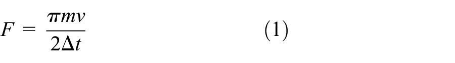
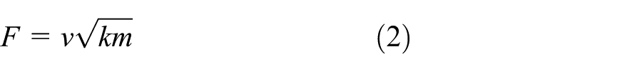
in which m is the total mass of the debris, v is the impact velocity, and Δt is the time to reduce the debris velocity to 0. Based on Haehnel and Daly (2004), FEMA P646 (2012) specifies a peak impact force given in equation (2), using the contact stiffness approach in which k is the effective contact stiffness of the debris and the structure

F = v \sqrt{k m}

(2)

The proper determination of Δt and k values is necessary to provide an accurate estimation of the peak impact force using impulse–momentum and contact stiffness approaches, respectively. Elastic axial debris impact test was conducted, and the experimental results were compared to the estimated values using the current design guidelines (Piran Aghl et al., 2013). The comparison indicated that the current design formulae are not consistent in the estimation of the impact forces, resulting in a lack of consensus on the specification of the design force. Additionally, the estimation methods provided by the current design guidelines do not explicitly account for the effect of magnitude and distribution of nonstructural mass (NSM) on impact demands. However, uniform distribution of mass along the entire length of the debris is unlikely especially for complex debris. Therefore, developing a model that accounts for the NSM is vital to predict accurately the debris impact demands.

In previous studies, the maximum impact forces from flood-borne woody debris were experimentally investigated and empirical formulae were proposed (Haehnel and Daly, 2002, 2004; Matsutomi, 2009). Numerical investigations have been carried out to evaluate the generated forces during shipping container impact on a reinforced concrete column (Madurapperuma and Wijeyewickrema, 2013). Formulae were obtained to estimate impact durations and effective contact stiffness (k) of concrete columns and shipping containers based solely on the simulation results. Previously, full-scale experimental studies have been conducted on a shipping container, wood utility pole, and steel tube to characterize the impact force demands generated during both axial and transverse debris impacts (Piran Aghl et al., 2014b, 2016). Additionally, simple analytical models were developed and validated with data from impact experiments to predict impact demands on the structures.

A one-dimensional (1D) model for impact force estimation of the debris under elastic response was developed based on a uniform bar model (Khowitar et al., 2014; Paczkowski et al., 2012; Piran Aghl et al., 2014b; Riggs et al., 2013). An inelastic response of the debris was also investigated and a simple analytical model was developed for estimation of the impact demands generated during inelastic response of the debris (Piran Aghl et al., 2014a). The estimation model was examined using numerical models and validated with experimental data. The results indicated that as the debris response changes from elastic to inelastic, the duration of the impact event increases and the peak impact force generated reaches a limit.

Previous research studies on the debris impact demands have been mainly focused on the debris without taking into account of the payload mass. Very limited work has been conducted to evaluate the effect of NSM on the debris impact forces. Linear numerical studies were carried out to investigate the effect of uniformly distributed NSM (payload mass) on impact demands of shipping containers under elastic response (Piran Aghl et al., 2014c). It was conservatively assumed that the additional uniform NSM is rigidly attached to the container. An equivalent 1D bar model was developed for the estimation of the elastic impact force in the case that NSM is rigidly attached to the debris.

More recent work was conducted to study the effect that supplemental uniform NSM attached to the debris has on the generated impact demands (Piran Aghl et al., 2015). Both experimental and numerical studies were carried out on a shipping container with uniform NSM mass. The effect of the impact velocity and magnitude of uniform NSM during both elastic and inelastic axial impact was numerically studied. A general approach was also developed using a simplified analytical model to provide an estimation of the axial impact demands of the uniformly loaded container.

Research effort has been previously made to better understand the effect of the uniform NSM on the debris impacts. However, non-uniform distribution of the NSM can significantly affect the debris impacts, and to the authors’ knowledge, there are no peer-reviewed research studies to examine this effect on the debris impact demands.

A small-scale model of the shipping container was tested in a wave flume to investigate the effect of water on the debris impact forces (Ko, 2013; Ko et al., 2014; Riggs et al., 2013). It was found that the contribution of water to the debris impact demands was secondary to the “pure” structural impact.

The objective of this study is to investigate the effect of non-uniform NSM distribution on axial debris impact under elastic and inelastic responses. This article presents an experimental program in which in-air axial impact tests were conducted on a component of a shipping container with rigidly attached non-uniform NSM. A steel tube is used to represent the main axial member of a shipping container and the attached NSM is representative of typical components connected to the member. The results are used to validate nonlinear dynamic finite element (FE) model that is extended for parametric evaluation. A simplified impact model is developed and validated by the experimental and simulation results to estimate the impact demands from the debris with non-uniform NSM.

Simplified 1D impact model

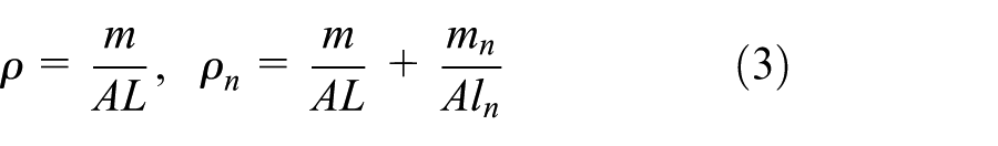
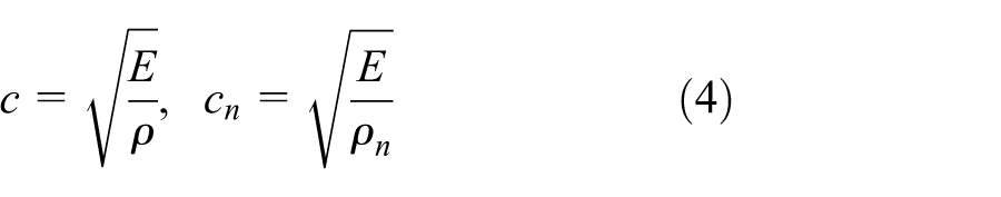
A simplified dynamic model is utilized based on the 1D stress wave theory to provide an accurate estimate of the axial impact demands of the debris with NSM. It is assumed that the longitudinal member of the debris that is subjected to an axial impact has a constant cross-sectional area along its entire length. The debris is modeled as an elastic bar of length L, cross-sectional area A, mass m, and elastic Young’s modulus E, subjected to axial impact at impact velocity v. Figure 1 shows a schematic of the 1D bar model impacting the rigid wall. The NSM m_n is assumed to be uniformly distributed over the length of 0 ≤ l_n ≤ L. The distance between the impact face and NSM is d > 0. The mass densities of the bar at the section without and with NSM (ρ and ρ_n, respectively) are given by equation (3). The elastic wave velocities (i.e. speed of sound) in the bar at the section without and with NSM (c and c_n, respectively) are given by equation (4)

ρ = \frac{m}{A L}, ρ_{n} = \frac{m}{A L} + \frac{m_{n}}{A l_{n}}

(3)

c = \sqrt{\frac{E}{ρ}}, c_{n} = \sqrt{\frac{E}{ρ_{n}}}

(4)

Figure 1.

One-dimensional impact model of debris with nonstructural mass (NSM).

When the debris strikes the wall, an acoustic wave propagates from the impact face to the free end of the debris (see Figure 1). The impact force for the uniform elastic bar is obtained from the solution of the 1D wave equation (Paczkowski et al., 2012). For a bar with varying densities, as presented in Figure 1, when the wavefront reaches the interface, part of the wave is reflected and part transmitted. The proportions of the incident wave that are reflected by the interface and transmitted to the second material are expressed by reflection and transmission coefficients, C_r and C_t, respectively (Achenbach, 1973). The coefficients are given by equation (5) for the bar presented in Figure 1, in which Γ is the ratio of the second material density to the first material density

C_{r} (Γ) = \frac{\sqrt{Γ} - 1}{\sqrt{Γ} + 1}, C_{t} (Γ) = \frac{2 \sqrt{Γ}}{\sqrt{Γ} + 1}

(5)

The initial impact force F₀ at the time t = 0 (when the initial stress wave starts propagating toward the free end of the bar) is

F_{0} = v c ρ A

(6)

The stress wave ratio (R) is defined as a ratio of stress waves returning to the impact face to the initial stress wave σ₀. Figure 2 shows the schematic representation of the propagation of a single wavefront for five different cases and defines the stress wave ratios for each case. Cases 1 and 2 represent the wave path for the first returning wave in compression and tension, respectively. In case 3, the initial wavefront propagates along the entire length of the debris, reflects back at the free end, and returns to the impact face. The stress wave ratios versus density ratios ρ_n/ρ are presented in Figure 3. It is shown that the stress wave ratio in case 1 (R₁) results in a compressive stress. Therefore, for case 1, the magnitude of the impact force increases when the returning wave reaches the impact face. This case represents the first compressive returning waves. The returning waves are fully reflected by the rigid wall (i.e. C_r = 1). Therefore, the reflected wave in case 1 propagates back and forth. In case 1, the impact force due to the reflected waves after the ith reflection from the wall is

^{(i)} F_{r} = 2 v c ρ A [\sum_{n = 1}^{i} {R_{1}}^{n}]

(7)

Figure 2.

Definition of stress wave ratios for different wave paths along the debris length.

Figure 3.

Comparison of stress wave ratios for different cases of returning waves.

Figure 3 indicates that the returning waves in cases 2–5 are tensile stresses, contributing to a reduction in magnitude of the impact force. For case 3, large proportion of the initial stress waves returns to the impact face at the corresponding time t₃ for relatively low values of the density ratio ρ_n/ρ. This results in a debris separation from the wall since the impact force becomes tensile. Figure 3 also shows that the tensile stress due to the returning wave in case 2 is larger than returning stress waves in cases 4 and 5. The first reduction in magnitude of the impact force is due to the returning wave in case 2 and can be determined as 2F₀R₂, where R₂ is the stress wave ratio in case 2. In Figure 4, the total impact force–time history is divided into three force histories: initial impact force F₀(t), the impact force due to returning waves in case 1 F_r(t), and the impact force due to returning waves in other cases F_t(t). The reflection time t_r and transmission time t_t are defined as the time taken to reach the impact face by the first reflected and transmitted waves, respectively (see equation (8)). In other words, t_r and t_t correspond to the traveling time for the wavefront in cases 1 and 2, respectively

t_{r} = \frac{2 d}{c}, t_{t} = 2 (\frac{d}{c} + \frac{l_{n}}{c_{n}})

(8)

Figure 4.

Idealized impact force–time history of debris with nonstructural mass using 1D model.

The peak impact force F_p illustrated in Figure 4 can be determined as

F_{p} = v c ρ A (1 + 2 \sum_{n = 1}^{N} {R_{1}}^{n})

(9)

in which N is the number of occurrences of a wave reflection from the wall within the time duration t_t. When d → 0 and therefore N → ∞, the asymptotic value of F_p is

F_{p} = v c ρ A \sqrt{\frac{ρ_{n}}{ρ}} = v c_{n} ρ_{n} A for N \to \infty

(10)

When the total impact force becomes tensile, the impact is over and the total duration can be computed. The total impact duration for a typical force history shown in Figure 4 is equal to t₃; however, for relatively high values of density ratio ρ_n/ρ,, the impact duration is sensitive to the location of NSM (i.e. d in Figure 1). For the constant values of m_n and t₃, increasing the distance between NSM and impact face leads to an increase in impact duration (Piran Aghl et al., 2014c). Since the 1D model presented in this article is developed for design applications, a simplified approach is used to estimate the impact force history. It is assumed that the impact force decreases at a constant rate after reaching the peak impact force at time t_t, as illustrated in Figure 4. To estimate impact duration, an impulse–momentum approach is used for the simplified 1D model. Since the elastic response is assumed herein, the total momentum of debris is 2(m + m_n)v. By equating the momentum with the area under the force–time history (i.e. impulse) of the simplified model presented in Figure 4, the debris impact duration t_d of the simplified 1D model can be estimated by

t_{d} = \frac{1}{F_{p}} [4 (m + m_{n}) v - 2 \int_{0}^{t_{t}} F (t) dt] + t_{t}

(11)

Experimental program

To investigate the effect of NSM on the debris impact demands, the experiments were conducted on a 6.1-m (20-ft) steel tube with different configurations of rigidly attached NSM under elastic response. A steel tube with approximately the same length and cross-sectional area as the longitudinal members of a standard shipping container was utilized in the experimental program to better understand the impact characteristics of the structural members of the complex debris. The steel tube was a standard American Institute of Steel Construction rectangular hollow structural section (HSS) of 64 × 38 × 4.8 mm with the measured cross-sectional area of 7.68 cm². The mass of the steel tube was 39 kg and the modulus of elasticity was taken to be 200 GPa.

Figure 5 illustrates the experimental impact setup developed to represent the head-on debris impact. The impact was generated using a pendulum system. A predetermined impact velocity was generated by raising the debris to the desired height prior to release. To provide uniform contact between the steel tube and load cell, a 7.6 × 5.1 × 1.3-cm plate was welded to the impact face of the steel tube, as shown in Figure 5.

Figure 5.

Experimental impact setup (cm).

To achieve sufficient resolution to accurately capture an impact event, data from all instrumentation (i.e. load cells, strain gauges, accelerometers, and light sensors) were recorded at 50 kHz. For each trial, impact velocity, force and duration from the load cell, and strain of the steel tube were measured.

A strain-based load cell was used to measure the impact force histories (see Figure 5). The global stiffness and frequency of the load cell provided by the manufacturer were 52,500 MN/m and 32 kHz, respectively. The first natural period of the load cell was well below the steel tube impact durations, resulting in an accurate representation of the impact forces by the load cell reading. The load cell was mounted on vertical members of the grillage and its location was adjusted to ensure axial impact of the steel tube along the center of the load cell. Dynamic analysis of the grillage subjected to the measured impact force histories at the location of the load cells revealed that the displacement of the grillage during debris impact duration is negligible. Therefore, the grillage can be assumed to act as a rigid structure in response to the steel tube impact.

Strain sensors were used to verify the measured impact force at the load cell and to assess stress wave propagation in the steel tube. The steel tube was instrumented with six resistance-based strain gauges at three cross sections along the length: 30 cm from the front, in the middle, and 30 cm from the rear. Each cross section was instrumented with two strain gauges at the top and bottom of the tube, as illustrated in Figure 5.

A light sensor was used to determine the impact velocity at the time of first contact between the steel tube and load cell. A slotted aluminum fin with perforations at a 1.27-cm spacing was attached under the steel tube (see Figure 5). The activation/deactivation of the light sensor was used to determine the time it takes to travel past each 1.27-cm perforation, thus allowing for calculation of the average velocity at impact. The fin was placed to allow for determination of velocity immediately prior to impact. The acceleration was also measured during the same time using accelerometers. The measured average velocity over the last slot and the acceleration averaged over the same time period were used to compute the velocity at impact (assuming constant acceleration).

A total of 63 trials were conducted on the steel tube with and without rigidly attached NSM. Steel plates were clamped along the length of the steel tube representing the rigidly attached NSM, as shown in Figure 5. Distribution of the NSM is achieved using lumped mass attachments. The distribution is described relative to a uniformity distribution index (UI) defined as

U I = 1 - \frac{l_{n} / s}{L}

(12)

in which s is the number of cross sections along the length l_n with assigned lumped mass attachments. L and l_n were previously illustrated in Figure 1. A value of UI = 1.0 indicates that the NSM is uniformly distributed along length l_n. UI = 0 represents a single lumped mass as an NSM distribution along the entire length L. The effect of distribution of NSM on the impact demands was assessed by conducting full and partial distributions of NSM along the length. Table 1 summarizes the test matrix for the steel tube experiments and provides the UI values corresponding to each test series. An NSM percentage, listed in Table 1, is defined as a percentage increase of the debris mass due to the additional NSM.

Table 1.

Test matrix for elastic axial impact of steel tube with NSM.

Test number	NSM distribution	Nonstructural mass^a (kg)	NSM %	s	UI	Impact velocity range (m/s)	Number of trials
T1	N/A	0	0	N/A	N/A	0.16–2.76	17
T2	Uniform—full length	20.6	53	4	0.75	0.56–2.85	11
T3	Uniform—full length	41.2	105	8	0.88	0.59–2.15	10
T4	Uniform—full length	75.0	192	10	0.90	0.9–2.24	5
T5	Uniform—full length	135.0	345	18	0.94	0.77–1.93	6
T6	Uniform—front half	20.6	53	4	0.88	0.84–2.59	10
T7	Uniform—back half	20.6	53	4	0.88	0.47–2.77	4

NSM: nonstructural mass; UI: uniformity distribution index; N/A: not available.

Nonstructural mass includes the total mass of the plates and clamping hardware.

FE modeling of steel tube impact

Numerical model

Three-dimensional nonlinear FE model of the steel tube with NSM was developed using ABAQUS Explicit 6.13 (Dassault Systems, n.d.) to investigate the effect of NSM distribution and nonlinearity on the impact demands. The impact simulations involved axial impact of the steel tube against a load cell, as illustrated in Figure 6. The impact force from FE analysis is determined from the contact force between the load cell model and the steel tube impact face.

Figure 6.

Steel tube and load cell mesh details and steel tube responses at 0.3 ms after impact.

The internal structure of the load cell body was not known. Consequently, the load cell body was modeled as a fictitious solid cylinder with a length equal to the overall load cell length. The constitutive properties were adjusted to result in the same fundamental frequency and stiffness reported by the manufacturer. The six-node solid wedge element (C3D6) is used for the load cell FE model.

An FE model of the steel tube specimen was created using the eight-node solid brick element (C3D8R). The point mass was defined at the locations of the clamping hardware to model the rigidly attached NSM along the length of the steel tube. The UI of 0.95 was used for NSM distribution in the parametric study. The location of lumped mass is shown in Figure 6. The material properties of the steel tube were mass density of 7850 kg/m³, Young’s modulus of 200 GPa, and Poisson’s ratio of 0.3. To assess the effect of nonlinearity on impact force, the measured plastic properties (true stress and true strain data) of the axial members of a standard shipping container (Piran Aghl et al., 2014a) were incorporated into the steel tube model; the yield strength and tensile strength were 381 and 519 MPa, respectively; the fracture strain was 25%. A contact definition was defined between the load cell and steel tube impact face using a Coulomb friction value of 0.21, which is a frictional coefficient for steel sliding on steel (Yuan et al., 2008). The self-contact was also defined in the steel tube model since the elements could be in contact under large deformations. Additionally, the steel tube model included strain rate effects by considering 10% increase in the strength of steel at the strain rate of 1/s (Piran Aghl et al., 2014a). The inelastic behavior of the FE model of steel components was previously validated against the full-scale shipping container experiments in Piran Aghl et al. (2014a).

Validation of numerical models

The impact force–time histories and strain–time histories from the elastic axial impact experiments are used to determine the accuracy of the impact simulations of the steel tube with NSM. The comparisons of force–time histories between the experiments and simulations with an impact velocity of 2 m/s for different NSM distributions are shown in Figure 7. It is seen that the peak impact force, duration, and overall force history response from the experiments and simulations are similar. Additionally, the measured strain–time histories from steel tube experiment T5 with 345% NSM at impact velocity of 2 m/s were compared to the strain–time histories from FE simulation, as shown in Figure 8. The comparisons indicate that the results of FE simulation of the steel tube with NSM correlate well with the experimental results.

Figure 7.

Comparison of impact force–time histories from experiments and simulations for steel tube with impact velocity of 2 m/s.

Figure 8.

Comparison of experimental data and simulation results for steel tube with 345% NSM at 2 m/s.

Experimental and numerical results

The peak impact force, impact duration, and impulse from the steel tube impact experiments and simulations are presented to investigate the effect of NSM magnitude and distribution on the impact demands. The results of FE simulations with impact velocities up to 3 m/s are described in this section to evaluate elastic response.

Figure 6 illustrates the stress wave propagation through the steel tube with and without NSM distribution at impact velocity of 4 m/s. Both stress distributions are shown at 0.3 ms after impact. As illustrated, the NSM distribution on the steel tube contributes to the reduction in stress wave speed. In addition, the reflected waves due to the presence of NSM lead to an increase in stress near the impact region. This behavior is consistent with the concept used for the 1D model presented in Figure 1.

To assess the effect of NSM on speed of sound through the steel tube, the wave speed was computed from the measured strain histories at two cross sections along the specimen (rear and front); the difference between the stress wave arrival time at strain gauge locations divided by the distance between two cross sections. Figure 9 compares the elastic wave speed from the experiments with different NSM magnitudes. It is evident that the increase in magnitude of rigidly attached NSM leads to a reduction in speed of sound.

Figure 9.

Effect of NSM on wave speed along the steel tube.

The relationship between the peak impact force and impact velocity for the steel tube with full and partial distributions of NSM are presented in Figures 10 and 11, respectively. The peak force varies linearly with the impact velocity for the steel tube with NSM. It can also be seen that the peak force increases as the magnitude of NSM increases, but it is sensitive to the location of NSM. For the given magnitude of NSM, the peak force increases as the NSM is distributed closer to the impact face.

Figure 10.

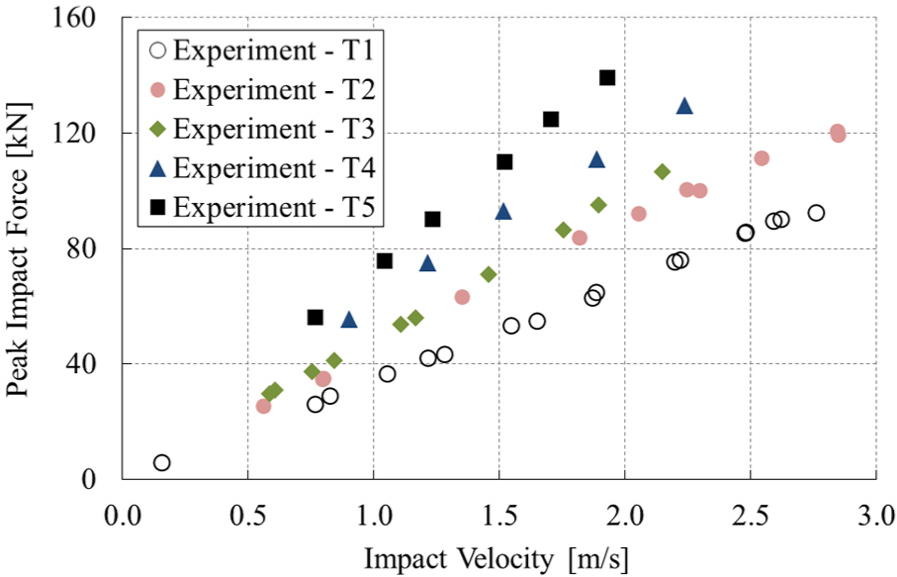
Peak impact force versus impact velocity for steel tube with full distribution of NSM.

Figure 11.

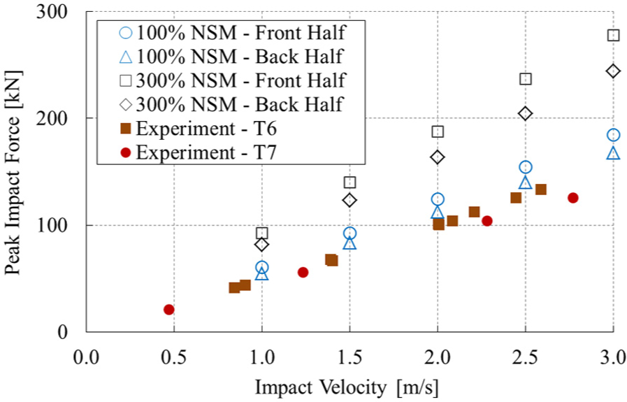
Peak impact force versus impact velocity for steel tube with partial distribution of NSM (front half and back half).

The impact duration of the steel tube experiments and simulations is defined as the time between the initial contact of the steel tube with the load cell and the end of the contact (i.e. when impact force becomes 0). The impact durations of steel tube versus impact velocity for full and partial distributions of NSM are shown in Figures 12 and 13, respectively. For all cases of NSM distribution, the impact duration remains constant over the range of impact velocities. The impact duration increases as the NSM increases. Figure 13 shows the effect of the location of NSM on impact duration. Both the experimental results (T6 and T7) and the simulation results show that the duration increases as the distance between the NSM and the impact face (i.e. d in Figure 1) increases.

Figure 12.

Impact duration versus impact velocity for steel tube with full distribution of NSM.

Figure 13.

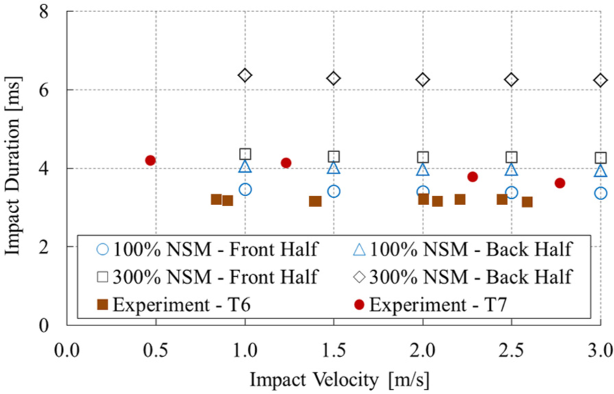
Impact duration versus impact velocity for steel tube with partial distribution of NSM.

The impulse (I) is defined as the area under the force–time history over the defined impact duration. The impulse values for the steel tube with different NSM distributions are plotted against the initial momentum (i.e. (m + m_n)v), as shown in Figure 14. The results are compared to the assumption used in the simplified 1D model (i.e. I = 2(m + m_n)v). The comparison indicates that the simplified 1D model provides a good approximation for the impulse.

Figure 14.

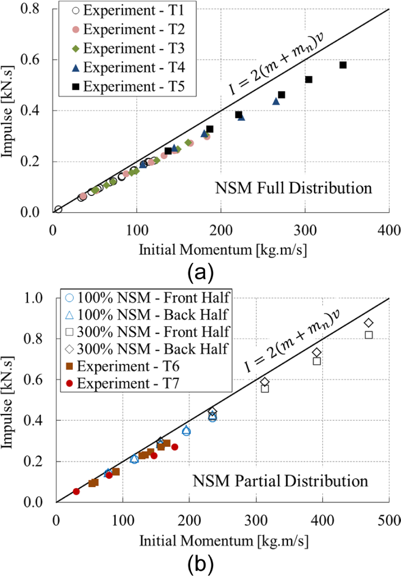
Relationship between impulse and momentum for steel tube with fully and partially distributed NSMs.

Impact force–time history estimation

In this section, the procedure outlined in Figure 4 for the simplified 1D model was used to estimate the impact demands. The lumped mass distribution along the full or partial length of the tube in the experiments and simulations provides a non-uniform distribution of NSM. However, to estimate impact demands using the 1D model, it is assumed that the NSM is distributed uniformly along the length l_n (see Figure 1). The accuracy of the 1D model is evaluated by comparison of the estimated values with the measured and simulated results. The measured and simulated peak impact force and impact duration have been nondimensionalized by the peak impact force and duration from the 1D model (equations (9) and (11), respectively). Note that equation (10) is used to estimate the peak force for impact cases with full and front half distributions of NSM (d ≈ 0).

The nondimensional peak impact force versus impact velocity is shown in Figure 15. The estimated values have been found to be in good agreement with the experimental and simulation results for steel tube with full and partial distributions of NSM.

Figure 15.

Nondimensionalized peak impact force versus impact velocity for steel tube tests and simulations.

Figure 16 presents the nondimensional impact duration at varying velocities for different magnitudes and distributions of NSM. The results show that the 1D model provides a reasonable approximation for impact duration. For NSM partial distribution, the impact durations for front half and back half distributions are slightly overestimated and underestimated by the 1D model, respectively.

Figure 16.

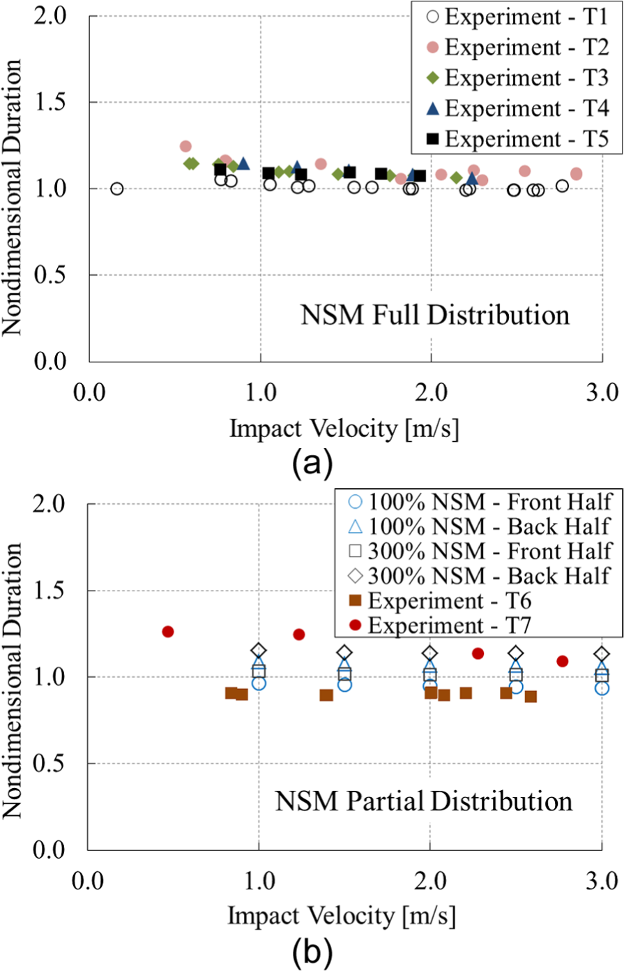
Nondimensionalized impact duration versus impact velocity for steel tube tests and simulations.

The estimated impact force–time history is compared to the measured and simulated force histories. Figure 17 shows the nondimensional force–time histories for different NSM magnitudes and distributions over a range of velocities. As illustrated, the estimated impact force–time histories by the simplified 1D model are in good agreement with the experimental and simulation results.

Figure 17.

Nondimensionalized impact force histories for the steel tube experiments and simulations and their comparison with the 1D model.

Effect of nonlinearity on impact forces

The impact simulations of the steel tube with impact velocities up to 30 m/s were conducted to assess the effect of nonlinearity on impact force, impact duration, and impulse. The steel tube consisted of 0%, 100%, and 300% NSM distributed along the entire length with the UI of 0.95 (s = 20).

The force–time histories for the impacts of the tube without NSM with initial velocities of 10, 20, 25, and 30 m/s are shown in Figure 18. As illustrated previously, when the reflected elastic wave reaches the impact face during elastic response, the total stress in the impact region becomes tensile and hence, the tube separates from the wall. Therefore, the impact duration does not vary with the impact velocity under elastic response. However, as the impact velocity increases and the material exceeds yield, the elastic stress wave is followed by plastic stress waves, which propagates at a lower speed. In this case, once the reflected elastic wave reaches the impact face (at time 2.5 ms), the total stress in the impact region still remains in compression because of the presence of compressive plastic wave. This results in an increase in impact duration, as shown in Figure 18.

Figure 18.

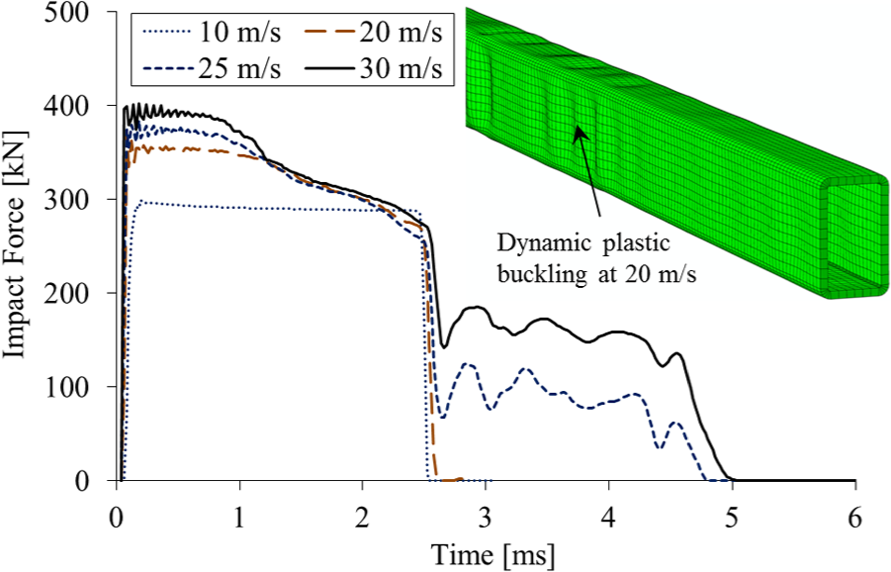
Impact force–time histories for inelastic axial impact of the steel tube without NSM.

Under inelastic response, the elastic and plastic waves start to propagate simultaneously from the impact face. Hence, the peak impact force occurs at the beginning of impact, as shown in Figure 18. This is followed by a reduction in the impact force due to occurrence of “dynamic plastic buckling” (Jones, 1989) of the tube section for relatively high impact velocities. The final buckled shape of the tube with impact velocity of 20 m/s is illustrated in Figure 18. It is also evident that the peak impact force increases as the impact velocity increases due to material strain hardening and it is not influenced by the occurrence of dynamic plastic buckling during impact event.

Figure 19 compares the peak impact force for the steel tube with and without NSM during inelastic response. The peak impact force increases as the magnitude of the NSM increases. However, the sensitivity to the magnitude of NSM decreases as the peak impact force is governed by the plastic response of the tube at higher impact velocities. Therefore, the peak impact force is not influenced by the NSM for relatively high impact velocities and it increases only due to the strain hardening of the tube without NSM.

Figure 19.

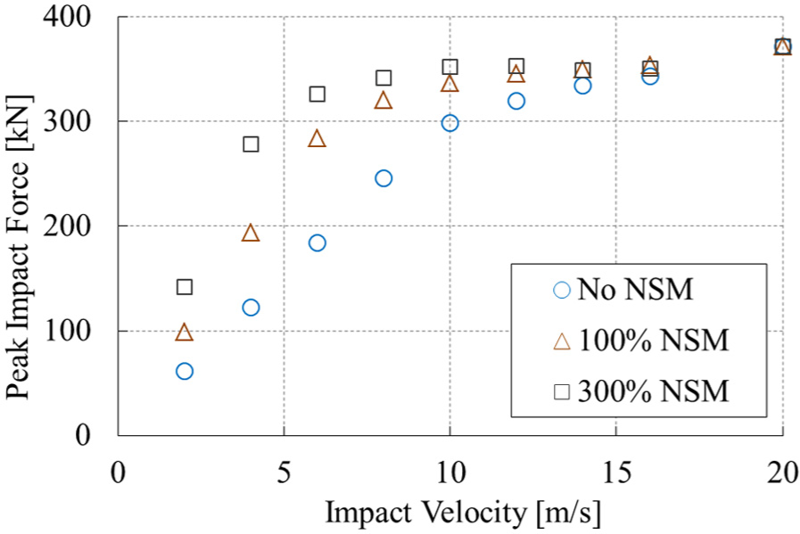
Peak force versus impact velocity for inelastic impact of steel tube with and without NSM.

The impact durations due to the impact of the steel tube with and without NSM are presented in Figure 20. For the steel tube with NSM, it can be seen that the impact duration remains constant for 100% and 300% NSM with impact velocities up to 12 and 8 m/s, respectively. For this range of velocities, the impact ends when the first reflection of the initial elastic wavefront from the wall occurs. For higher impact velocities, the impact duration increases as a result of inelasticity.

Figure 20.

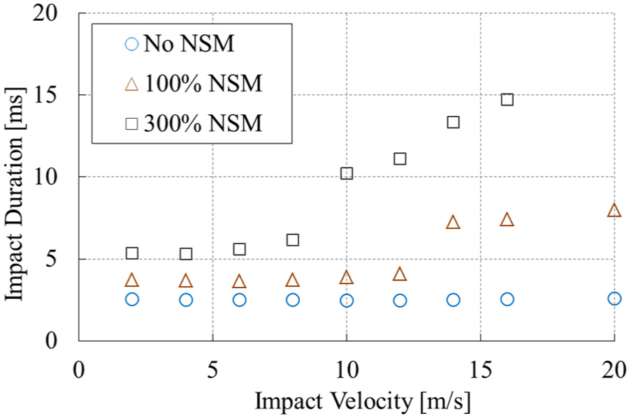
Impact duration versus impact velocity for inelastic impact of steel tube with and without NSM.

The relationship between the impulse and impact velocity is shown in Figure 21. It is evident that the impulse values are bounded between (m + m_n)v and 2(m + m_n)v. For high impact velocities, a considerable portion of the impact energy is absorbed by the plastic deformation of the tube, contributing to a reduction in impulse. In this case, the rebound velocity of the tube tends to be 0 (i.e. coefficient of restitution is equal to 0).

Figure 21.

Impulse versus impact velocity for inelastic impact of steel tube with and without NSM.

Conclusion

In this article, a simplified 1D model is developed to estimate the force–time history generated from an axial impact of the elastic debris. The proposed model accounts for the location and magnitude of the NSM attached along the length of the debris. The stress wave propagation in a 1D bar and impulse–momentum approach are used to estimate the peak impact force and impact duration, respectively.

A series of experiments on a 6.1-m steel tube with different configurations of rigidly attached NSM were carried out under elastic response. A three-dimensional nonlinear dynamic FE model of the steel tube with NSM was developed and validated with the results from the experiments. The impact simulations consisted of elastic and inelastic impacts of the tube with NSM.

The experimental and simulation results were used to validate the 1D model. It is found that the 1D model provides a good agreement for the peak impact force and impact duration and gives a conservative estimate of impulse. In addition, the estimated pulse shape correlates well with the measured and simulated results.

The results indicate that the peak impact force is influenced by the location of NSM and it can be well estimated by the 1D model. Also, it is shown that the peak impact force is not affected by the NSM under inelastic response. The simplified 1D model can be used to characterize the impact demands from debris with uniform and non-uniform nonstructural components.

Footnotes

Declaration of Conflicting Interests

The author(s) declared no potential conflicts of interest with respect to the research, authorship, and/or publication of this article.

Funding

The author(s) disclosed receipt of the following financial support for the research, authorship, and/or publication of this article: This material is based on the work supported by the National Science Foundation (NSF) through the NSF George E. Brown, Jr. Network for Earthquake Engineering Simulation (grant CMMI-1041666). This funding is gratefully acknowledged.

References

Achenbach

(1973) Wave Propagation in Elastic Solids. Amsterdam: North Holland.

American Society of Civil Engineers (ASCE) 7 (2010) Minimum Design Loads for Buildings and Other Structures (ASCE/SEI 7-10). Reston, VA: ASCE.

Dassault Systems (n.d.) Abaqus Unified FEA Software, version 6.13. Providence, RI: Dassault Systems (SIMULIA Corp).

Federal Emergency Management Agency (FEMA P55) (2011) Coastal Construction Manual, vol. 2. 4th ed.Washington, DC: FEMA.

Federal Emergency Management Agency (FEMA P646) (2012) Guidelines for Design of Structures for Vertical Evacuation from Tsunamis. 2nd ed.Washington, DC: FEMA.

Fraser

Raby

Pomonis

. (2013) Tsunami damage to coastal defences and buildings in the March 11th 2011 Mw 9.0 Great East Japan earthquake and tsunami. Bulletin of Earthquake Engineering11(1): 205–239.

Haehnel

Daly

(2002) Maximum impact force of woody debris on floodplain structures. ERDC/CRREL TR-02-2. February 2002. Vicksburg, MS: US Army Corp of Engineers, Engineer Research and Development Center. Available at: http://acwc.sdp.sirsi.net/client/search/asset/1001598

Haehnel

Daly

(2004) Maximum impact force of woody debris on floodplain structures. Journal of Hydraulic Engineering130(2): 112–120.

Jones

(1989) Structural Impact. Cambridge: Cambridge University Press.

10.

Khowitar

Riggs

Kobayashi

(2014) Beam response to longitudinal impact by a pole. Journal of Engineering Mechanics. Available at: http://ascelibrary.org/doi/abs/10.1061/(ASCE)EM.1943-7889.0000765

11.

. (2013) Hydraulic experiments on impact forces from tsunami-driven debris. Master Thesis, Department of Civil and Construction Engineering, Oregon State University, Corvallis, OR.

12.

Cox

Riggs

. (2014) Hydraulic experiments on impact forces from tsunami-driven debris. Journal of Waterway, Port, Coastal, and Ocean Engineering. Available at: http://ascelibrary.org/doi/abs/10.1061/(ASCE)WW.1943-5460.0000286

13.

Madurapperuma

MAKM

Wijeyewickrema

(2013) Response of reinforced concrete columns impacted by tsunami dispersed 20 and 40 shipping containers. Engineering Structures56: 1631–1644.

14.

Matsutomi

(2009) Method for estimating collision force of driftwood accompanying tsunami inundation flow. Journal of Disaster Research4(6): 435–440.

15.

Naito

Cercone

Riggs

. (2013) A procedure for site assessment of the potential for tsunami debris impact. Journal of Waterway, Port, Coastal, and Ocean Engineering140: 223–232.

16.

Paczkowski

Riggs

Naito

. (2012) A one-dimensional model for impact forces resulting from high mass, low velocity debris. Structural Engineering and Mechanics42(6): 831–847.

17.

Piran Aghl

Naito

Riggs

(2013) An experimental study of demands resulting from in-air impact of debris. In: Proceedings of the 11th international conference on structural safety and reliability, New York, 16–20 June, pp. 5541–5547. London: Taylor & Francis.

18.

Piran Aghl

Naito

Riggs

(2014a) Estimation of demands generated from axial impact of steel debris under inelastic response. Engineering Structures82(1): 11–21.

19.

Piran Aghl

Naito

Riggs

(2014b) Full-scale experimental study of impact demands resulting from high mass, low velocity debris. Journal of Structural Engineering140(5): 04014006.

20.

Piran Aghl

Naito

Riggs

(2014c) Investigating the effect of nonstructural mass on impact forces from elastic debris. In: Proceedings of the ASCE Structures Congress, Boston, MA, 3–5 April, pp. 635–644. ASCE, DOI: 10.1061/9780784413357.057.

21.

Piran Aghl

Naito

Riggs

(2015) Effect of nonstructural mass on debris impact demands: experimental and simulation studies. Engineering Structures88(4): 163–175.

22.

Piran Aghl

Naito

Riggs

(2016) Study of demands resulting from transverse impact of high mass, low velocity debris. Advances in Structural Engineering19: 1328–1344.

23.

Riggs

Cox

Naito

. (2013) Water-driven debris impact forces on structures: experimental and theoretical program. In: Proceedings of the ASME 2013/32nd international conference on ocean, offshore and Arctic engineering, Nantes, 9–14 June, OMAE2013-11128. New York: ASME.

24.

Robertson

Carden

Riggs

. (2010) Reconnaissance following the September 29, 2009 tsunami in Samoa. UHM/CEE10-01. Honolulu, HI: University of Hawaii. Available at: http://cee.hawaii.edu/reports/UHM-CEE-10-01.pdf

25.

Robertson

Chock

Morla

(2012) Structural analysis of selected failures caused by the 27 February 2010 Chile tsunami. Earthquake Spectra28(S1): 215–243.

26.

Robertson

Riggs

Yim

SCS

. (2007) Lessons from hurricane Katrina storm surge on bridges and buildings. Journal of Waterway, Port, Coastal, and Ocean Engineering133(6): 463–483.

27.

Yuan

Harik

Davidson

(2008) Multi-Barge Flotilla Impact Forces on Bridges. Lexington, KY: University of Kentucky.