Wind tunnel test and numerical simulation of wind characteristics at a bridge site in mountainous terrain

Abstract

Wind tunnel test and computational fluid dynamics simulation were conducted to study the wind characteristics at a bridge site in mountainous terrain. The upstream terrains were classified into three types: open terrain, open terrain with a steep slope close to the bridge, and open terrain with a ridge close to the bridge. Results obtained from the two methods were compared, including mean speed profiles in the vertical direction and variations of wind speed and angle of attack along the bridge deck. In addition, turbulence intensities at the bridge site obtained from wind tunnel test were discussed. For mean speed profiles in the vertical direction, two methods are reasonably close for open terrain, while mountain shielding effects are evident for open terrain with a steep slope for both the methods, but the extents of effects appear different. Wind speed and angle of attack along the bridge deck are mainly influenced by the local terrain. Strong downslope wind is generated at the lee slope for the case of wind normal to top of the ridge. The comparative results are expected to provide useful references for the study of wind characteristics in mountainous terrain in the future.

Keywords

angle of attack bridge site computational fluid dynamics simulation mean wind speed mountainous terrain turbulence intensity wind characteristics wind tunnel test

Introduction

Since bridges have become more and more flexible with the increasingly long spans, wind-resistant problems of the bridges have become more important. As a fundamental issue on wind-induced responses of bridges, the research on wind characteristics at bridge sites is essential. Wind characteristics are comparatively uniform for coastal or open terrain and can refer to specifications or previous studies. However, when dealing with the mountainous terrain, wind characteristics are significantly different. It is well known that there are various mountains and gorges in southwest and northwest China, and with the implementation of the western development strategy, more and more bridges in mountainous terrain are about to be built. Hence, it is urgent to conduct the research on the wind characteristics at bridge sites in mountainous terrain, to provide information in wind disaster mitigations of the bridges in the complex areas.

Several methods are available for the measurement of wind characteristics, which are basically field measurement (Chen et al., 2007; Tamura et al., 2007; Ucar and Balo, 2009; Xu et al., 2000), wind tunnel test (Carpenter and Locke, 1999; Derickson and Peterka, 2004; Sierputowski et al., 1995), and computational fluid dynamics (CFD) simulation (Huang and Xu, 2013; Li et al., 2011; Paterson and Holmes, 1993). These methods are applied in many cases, involving mountainous terrains as well.

Tests in a boundary layer wind tunnel (BLWT) possess the advantages of easy control and short cycle, which have been used broadly. Meroney (1980) evaluated the accuracy of the wind tunnel investigation on flow over a complex terrain model, where both terraced and contoured models were used. The effects of topography on the design loads for long-span bridges were studied by Davenport and King (1990) through three examples, from which large spatial variations in mean wind velocity were observed along the bridge deck for the sheltered exposure. Derickson and Peterka (2004) carried out BLWT tests using a 1:4000 scale model of a complex terrain covering an area of 225 km² in the wind tunnel, of which each terrace step has 12 vertical meters for the actual topography. Li et al. (2010) performed BLWT tests with four simplified valley models and a 1:500 scale model of a real terrain at the mountain bridge site, and speed-up effects were observed. The influences of model scale on the BLWT simulation of complex terrain were discussed by Neal (1983), in which simulations with 1:4000 and 1:8000 models were conducted and compared with the full-scale measurement. In the above investigations, there is a high degree of compatibility, demonstrating that the wind tunnel test is a feasible method.

Although a BLWT test is a recognized method of investigating wind characteristics, CFD simulation method tends to become a feasible alternative approach. With the advancement of computational techniques, the CFD method is rapidly developing and widely used in the studies of wind characteristics. Besides, if the wind characteristics are known in the early designs by CFD method, the sites of bridge and configurations of structures could get optimized, and thus considerable investment would be saved. A finite difference method was used to develop simulation codes by Uchida and Ohya (1999), and flow over a real complex terrain was calculated where strong influences on the surface winds by the topography were found. Li et al. (2011) carried out a numerical simulation for the wind field distribution of bridge site with complex terrain to explore the spatial distribution feature of the wind field over the bridge site, and the research provided a basis for the determination of design wind speed of the bridge.

It is still of significant importance for the comparison study of wind tunnel test and CFD simulation for the wind characteristics in the mountainous terrain. Comparison between the two methods is the key point in the article, to provide references for wind characteristics in mountainous terrain. A series of investigations have been carried out to study the wind characteristics at a bridge site in mountainous terrain. The investigated terrain is representative, for the upstream terrains around the bridge include open terrain with a steep slope and open terrain with a ridge. The bridge is located halfway up the gorge of the mountain, which is 250 m high above the river, and the mean altitude of the bridge deck is 1608 m. The highest altitude for the terrain within a 10 km diameter range reaches over 4600 m. Studies on the wind characteristics at the typical bridge site in mountainous terrain were conducted by wind tunnel test and CFD simulation. Results from the two methods were discussed in detail. Some conclusions can be drawn in the following.

Wind tunnel test

Physical model in the wind tunnel

The tests were carried out in the XNJD-3 wind tunnel. It is a return-circuit type of wind tunnel with a cross section of 22.5 m wide and 4.5 m high. The physical model in the wind tunnel test for wind characteristics at the bridge site consisted of four main parts: terrain model, boundary transition sections, rotary platform, and testing supports.

In the wind tunnel test, the terrain model was made with a large scale of 1:2000 to consider the topographic changes around the bridge site and the width and height of the wind tunnel comprehensively. The altitude in the considered actual terrain ranged from 1360 to 4800 m. The bottom of the model was defined as the surface of the river, and the maximum height of the terrain model was about 1.72 m. The bridge was situated at the center of the model. Terrace models with both 10 and 5 mm height intervals were used, which represented 20 and 10 m height intervals of the actual terrain. Terrace steps of 5 mm were used near the bridge site for the purpose of refining the most concerning area, while 10 mm terrace steps were used in the area far from the bridge site. The manufactured terrain model is shown in Figure 1.

Figure 1.

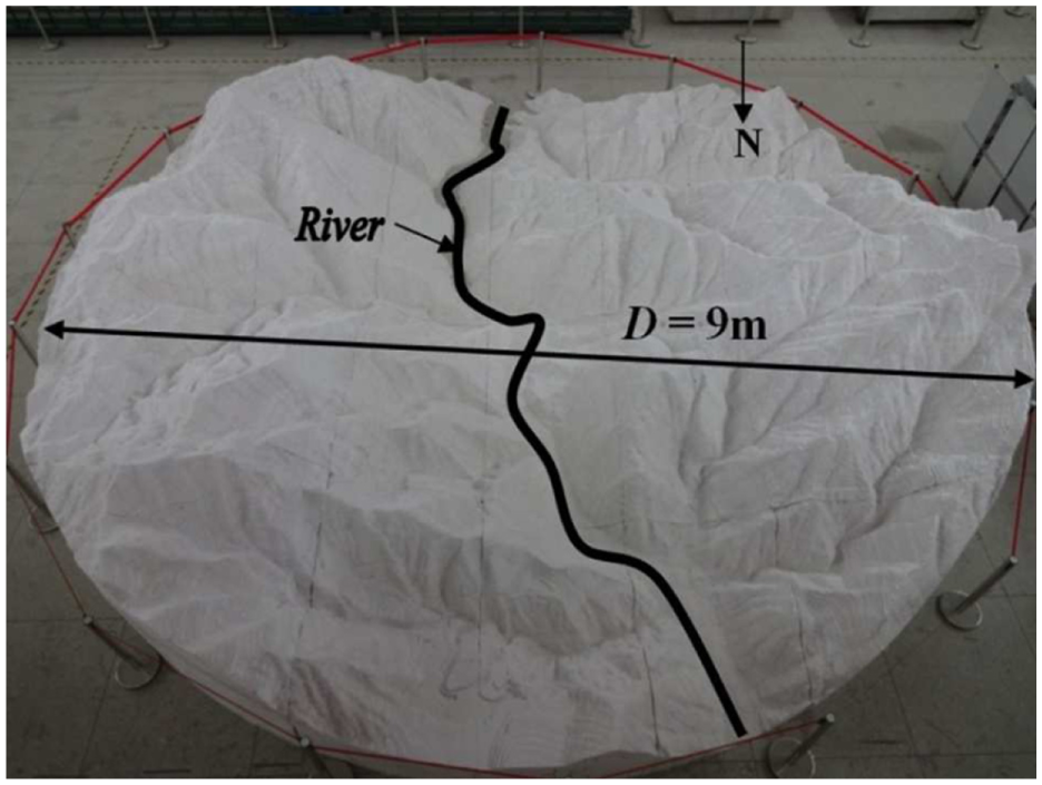
1:2000 scale physical terrain model in the BLWT.

The effectiveness of the transition for the terrain was examined by Utsunomiya et al. (1989), showing that the transition section was able to decrease the limitations of scale problems effectively. With regard to the mountainous terrain, transition sections at the edges of the terrain model were required. In general, linear transitions were commonly used in the past studies. But if the edges of the mountains are too high, the linear transitions would lead to apparent flow separations. Hence, it is essential to arrange the reasonable boundary transition sections around the terrain model, especially for the mountainous terrain, to obtain more reliable test results. The shapes of the boundary transition sections were calculated following the paper by Hu et al. (2015), which were deduced based on the theory of ideal fluid flow around a cylinder. On account of the undulating changes of the model edge, non-uniform cross sections of the boundary transition sections were used in different positions. To fully consider the altitude changes and conveniently assemble these sections, the terrain edge is divided to 47 key sections (Figure 2(a)), of which a typical section is displayed in Figure 2(b).

Figure 2.

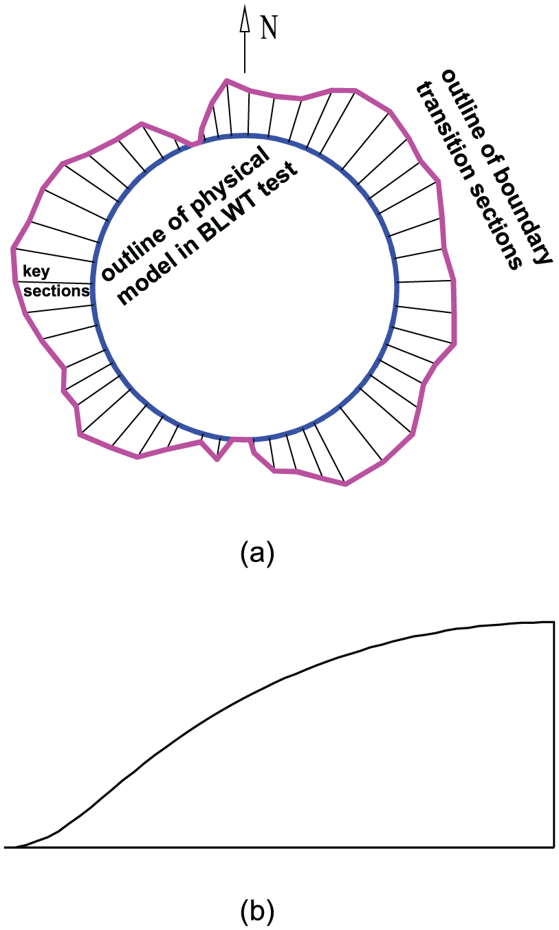
Boundary transition sections in the BLWT: (a) overall view of boundary transition sections and (b) typical cross section of key sections.

For the sake of changing incoming flow directions, a rotary platform with a diameter of 9 m was manufactured so that the terrain model could be rotated easily. Manual testing supports were utilized, in order to move the test probes horizontally and vertically in a wide range. Both spires and roughness blocks were used to generate the boundary layer, as shown in Figure 3. The atmospheric boundary layer in the wind tunnel was simulated according to type IV, which represents very rough terrain, in the Chinese design code (wind-resistant design specification for highway bridges; JTG/T D60-01-2004, 2004). The power exponent coefficient α = 0.296, which is consistent with α = 0.3 stipulated in the design code.

Figure 3.

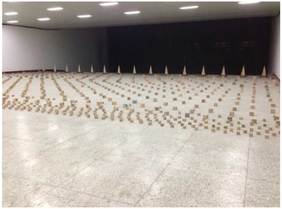
Turbulent generators in the BLWT.

Data acquisition and processing method in the wind tunnel test

The TFI Cobra Probe was utilized in the wind tunnel test, which outputs raw voltage data. The data were converted to speed data by TFI Device Control software. In the study, the sampling frequency of the probe was set as 1250 Hz, and the sampling time was 120 s. The model was tested in the turbulent boundary layer flow. The speed at 2.1 m high position of the mid-span above the river surface in the test was regarded as the gradient wind speed u_G, by which all the data were normalized.

Mean wind speed is the average of wind speed in 120 s tested in the BLWT tests. It includes three components: transverse, bridge-axial, and vertical wind speeds, represented by u, v, and w, respectively. The vertical wind angle of attack is defined in equation (1). A positive angle of attack indicates that the flow is upward and vice versa

α = \tan^{- 1} \frac{w}{| u |}

(1)

CFD simulation

CFD numerical model

The CFD software FLUENT was utilized to simulate the wind characteristics at the bridge site. The geometry of the flow region was established in the pre-procession software GAMBIT. The simulation region covered an area of 400 km² (20 km from north to south and 20 km from east to west), and the center was positioned at the bridge site. The altitude of the simulated region reached 15,000 m. Hence, the air above the surface had plenty space to flow freely. The bottom of the region was generated by the terrain contour lines and was set as wall boundary and smoothly transited. The overhead view of numerical model is shown in Figure 4(a), in which the line represents the bridge axis. The model region was discretized using tetrahedral unstructured grids. To refine the region around the bridge site, the area contained a high density of cells. The grid sensitivity analysis was checked by some comparative investigations, and then the total number of cells was determined to be about 2.31 million, and the minimum mesh size is about 8 m, which can meet the requirements (Figure 4(b)). It is noted that different methods have their own requirements on the models, so it is not reasonable to utilize the exact same model. To compare the two methods, an area of about 400 km² is used for analysis, which is large for the gradual transition and free movement of the air flow. Hence, the effects of the model size and inlet boundary on the concerned area of the two models are likely to be weakened.

Figure 4.

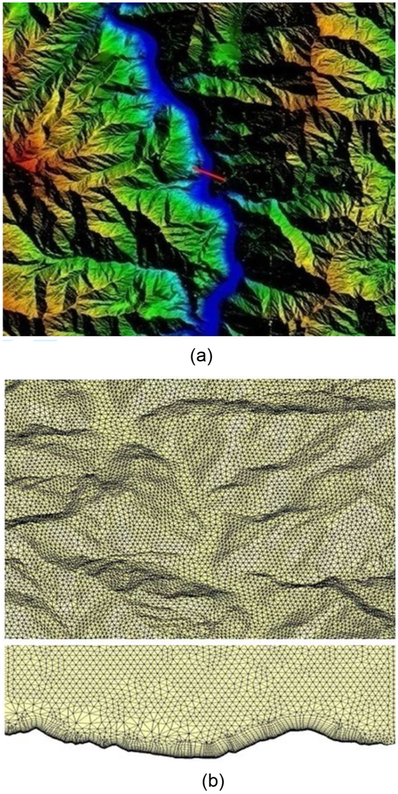
CFD numerical model: (a) overall view and (b) local grid.

CFD simulation parameters

In the CFD simulation, the finite volume method was utilized in the discretization of the governing equations. The shear stress transport (SST) k-ω model developed by Menter (1994) was used for the turbulence model. The SST k-ω turbulence model integrates the superiorities of the original k-ω in the near wall layer and the free stream independence of the standard k-ε model in the outer region. The pressure-based solver and the implicit formulation were used, which were suitable for incompressible flow. The Semi-Implicit Method for Pressure-Linked Equations - Consistent (SIMPLEC) algorithm was applied to the pressure–velocity coupling, the second-order interpolation scheme was adopted for pressure, and the second-order upwind scheme was used for the moment and turbulence properties.

The inlet velocities were set up by user-defined function (UDF) and are given in equation (2), and the height of gradient wind for the inlet was taken as 3000 m. The inlet and outlet conditions were required to be set corresponding to each case. In the simulation, all the outlets were set as pressure outlet. In the setting process, the monitoring points were arranged along, above, and below the bridge axis. To judge the convergence, a residual of 10⁻⁶ on all variables is set

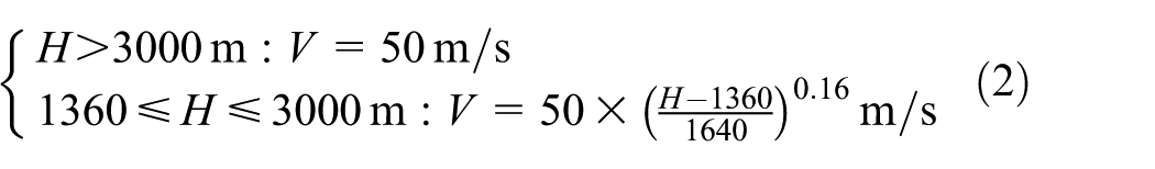
{\begin{matrix} H > 3000 m : V = 50 m / s \\ 1360 ⩽ H ⩽ 3000 m : V = 50 \times {(\frac{H - 1360}{1640})}^{0.16} m / s \end{matrix}

(2)

where H represents the altitude and V represents the inlet velocity.

Data processing method in CFD simulation

Wind speeds in x-, y-, and z-directions were obtained from the FLUENT, and the speeds in x- and y-directions were transformed to transverse and bridge-axial wind speeds, namely, u and v. The angle of attack was calculated using equation (1).

Results and discussion

Case description

In order to attain the mean speed profiles in the vertical direction at the bridge site, monitoring points were set at the mid-span vertically. In addition, to attain variations of wind speed and angle of attack along the bridge deck, seven equally spaced monitoring points were arranged.

The focal points of the study are to attain the mean wind speed profiles in vertical direction, and the variations of wind speed and angle of attack along the deck. To compare the wind speeds from the two methods in different cases more intuitively, ratio of wind speed at a certain height u to gradient wind speed u_G was adopted. Furthermore, turbulence intensity at the bridge site was obtained in the BLWT test, to show the turbulence features.

Taking full consideration of the circumstances around the bridge site and the prevailing wind directions, six wind directions were investigated as shown in Figure 5, where the numbers represent the testing cases. The inflow is categorized into two kinds according to the wind direction: north wind and south wind. The wind directions for Cases 2 and 6 are normal to the bridge axis. The wind directions of Cases 1 and 5 are along the local river at the bridge site. The direction for Case 4 is approximately consistent with the overall river direction. It is noted that wind direction for Case 3 is normal to the southeastern ridge in front of the bridge.

Figure 5.

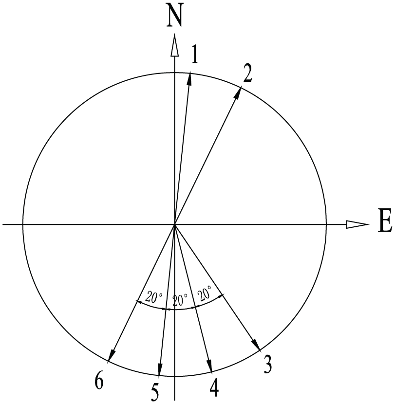
Wind directions of the investigated cases.

The investigated bridge site is typical, for it includes several mountainous topographies, which are open terrain (hereinafter referred to as Type 1), open terrain with a steep slope close to the bridge (Type 2), and open terrain with a ridge close to the bridge (Type 3). The three types of upstream terrains are illustrated in Figure 6.

Figure 6.

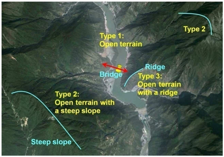
Three types of the upstream terrains (topography excerpted from Google Earth).

Mean speed profiles in the vertical direction

Comparative study of the mean speed profiles in the vertical direction focused on four cases (Cases 1, 2, 5, and 6). Here, Case 1 corresponds to Type 1, while Cases 2, 5, and 6 correspond to Type 2.

Figure 7 shows the mean vertical speed profiles for four cases at the mid-span of the bridge from both the BLWT test and the CFD simulation. The abscissa is the ratio of u to u_G. The results are reasonably close for Case 1 from the two methods since the upstream terrain is little sheltered. Meanwhile, it is shown that the results from the CFD method are a little larger than those from the BLWT test, which may be caused by the fact that the terrain of the CFD simulation changed smoothly while that of the BLWT test was terraced. In general, the SST k-ω model performed well for the open terrain. As for the other three cases (Type 2), steep slopes are situated 2–3 km far from the bridge site, which produce about 1300 m altitude difference to the maximum. The results from the two methods reflect the shielding effects of the high mountains. However, the extents of the shielding effects appear different for the two methods especially in the low altitude, and the differences are mitigated with the altitude increasing.

Figure 7.

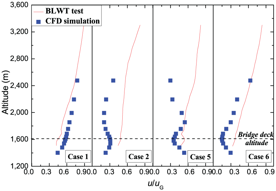
Mean speed profiles in the vertical direction at the mid-span of the bridge.

An inflection point is observed in the CFD simulation for Case 5. As illustrated above, the shielding effects of the two methods are likely to be different. As for Case 5, the wind velocity in the low altitude is influenced mainly by the local terrain, while that in the high altitude is by both local terrain and leading wind direction. The leading direction of the air flow for Case 5 is northeast (Figure 5). But the direction of the local river in the upstream of bridge site is northwest, and the air flow may be guided by the local river in the northwestern direction and by the ridge from the low altitude to high altitude. Hence, in CFD simulation, the air flows from the opposite directions meet in the high altitude, leading to the low wind velocity and the inflection point. Moreover, streamlines of wind speed for Case 5 are shown in Figure 8, which indicates that the inflection point partially results from effects of the flow separation caused by the upstream mountains and by the local river in the CFD simulation.

Figure 8.

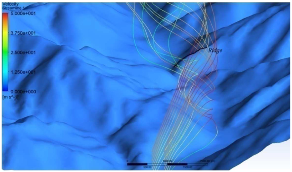
Streamlines of wind speed for Case 5 at the bridge site from CFD simulation.

The profiles are not regular in a low altitude for all these cases, demonstrating that the wind is greatly influenced by the local terrain. As the bridge is intended to be constructed halfway up the gorge, the wind direction and local terrain have direct effects on wind profiles at the bridge site. Unlike the open or coastal terrain, most of the profiles in mountain terrains do not follow a power or logarithmic law, as shown by the results from both methods.

Variation of mean wind speed along the bridge deck

As the distributions have significant influences on the wind loads on the bridges, studies of the wind speed distributions along the bridge axis are essential for long-span bridges. To discuss the differences of the two methods, four cases mentioned above were tested. Results are shown in Figure 9. It is observed that the mean wind speeds from the two methods along the bridge axis are close for Case 1. Similar to the wind speed profiles in the vertical direction, mean wind speeds along the bridge deck from CFD simulation are slightly larger than those from the BLWT test. Due to rapidly changing terrain at the southeastern side of the bridge site, large variations are found in Cases 5 and 6. The results of three monitoring points on the eastern side vary much more sharply in the CFD simulation, indicating that the extents of the shielding effects of greatly changing terrains are different for the two methods.

Figure 9.

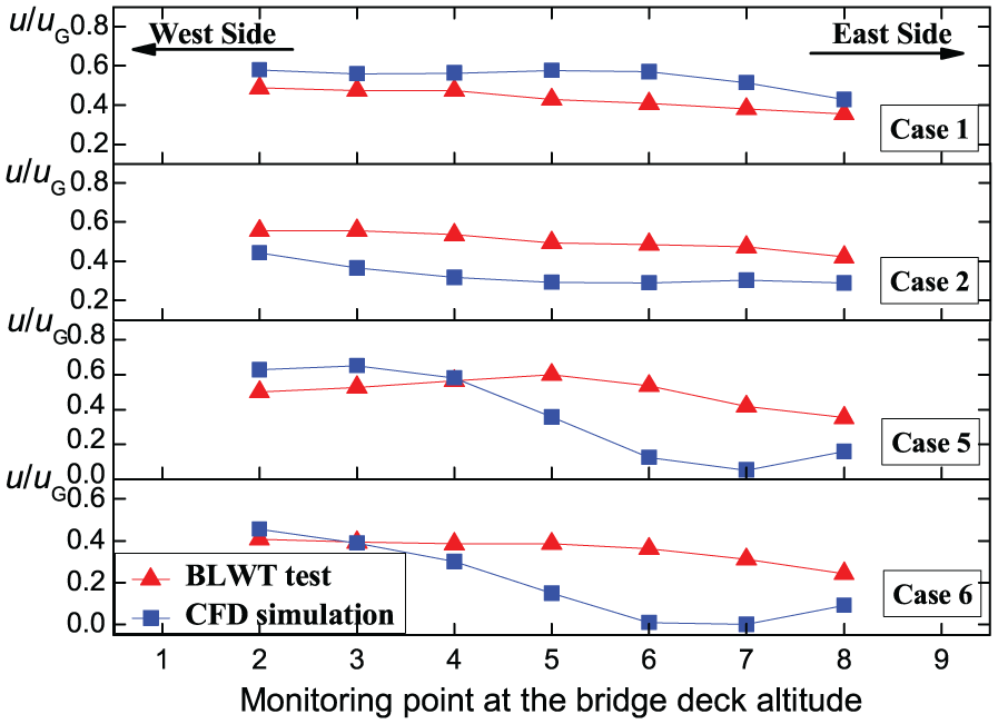
Mean wind speed along the bridge deck (Types 1 and 2).

Variation of angle of attack along the bridge deck

In the wind-resistant designs of bridges, angles of attack have great influences on the wind-induced behaviors of bridges. Angle of attack in mountainous terrain is changeable spatially, which differs from the features in coastal terrain.

The above four typical cases were adopted to compare the distributions of angle of attack along the bridge deck, shown in Figure 10. The differences between the two methods are small for Case 1. Similar to the variations of mean wind speed along the deck, the angles of attack of three eastern monitoring points are greatly influenced by the local terrain and the discrepancies are generated between the two methods. However, the discrepancies appear much more apparent for the south wind cases (Cases 5 and 6), and angles of attack of the three eastern points are too large due to very low wind speeds in CFD simulation (dashed frame in Figure 10), which may result from the measurement error and the effects of local grid and terrain. But it should be noted that it is not a controlling case when the wind speed is too low.

Figure 10.

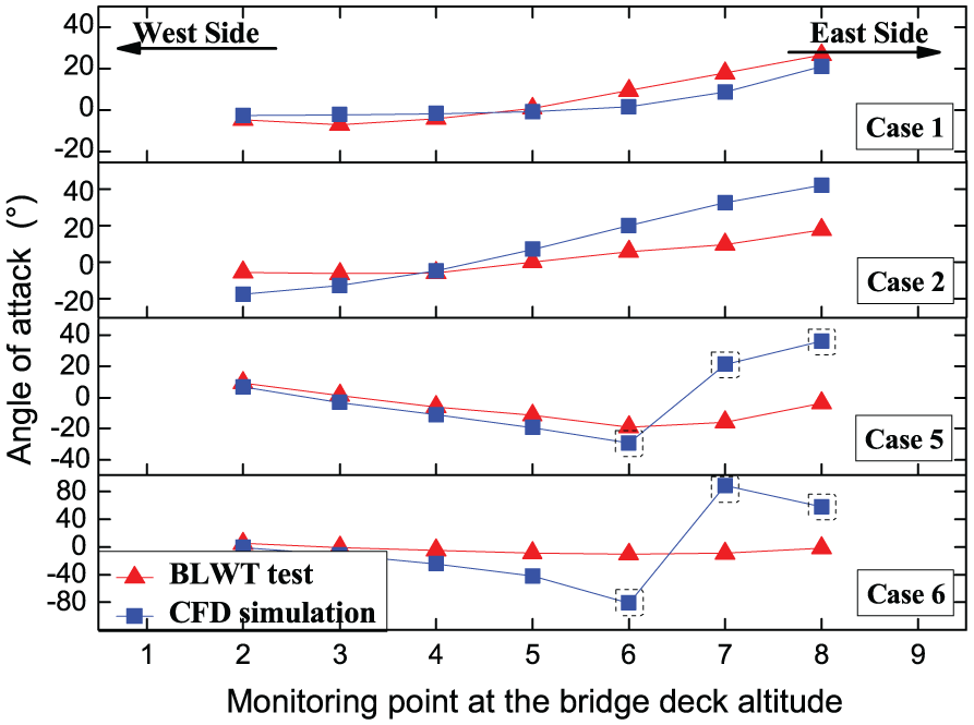
Angle of attack along the bridge deck (Types 1 and 2).

Effects due to ridges

As observed in the above study, the southeastern terrain at the bridge site is complex for the local river bend and the ridge exposure. Hence, to study the effects caused by the ridge located in the upstream terrain of the bridge site (Type 3), Cases 3 and 4 are investigated.

Although the angle between two cases is 20°, it is actually two different situations. For Case 3, the incoming flow is normal to top of the ridge, while for Case 4, the flow is approximately along the ridge. The variations of mean wind speed and angle of attack along the bridge deck are shown in Figures 11 and 12, respectively. Results show similar characteristics for the two cases. For Case 3, wind speeds of three eastern points are comparatively large, and large negative angles of attack were observed. It is supposed that strong downslope wind is generated at the lee slope after flowing over the ridge top. However, when wind arises along the ridge for Case 4, positive angles of attack are formed and significant mountain shielding effects are observed. Due to the ridge, large variations in mean wind speed are noticed along the bridge deck. With regard to the angle of attack for Case 4, since the wind speeds of three eastern points are quite low, angles of attack are too large in CFD simulation (dashed frame in Figure 12), which may result from the measurement error and the effects of local grid and terrain. But it is not a controlling case, for the wind speeds are too low. It is worth noting that the non-uniform wind loads on the bridge deck should be paid sufficient attention.

Figure 11.

Mean wind speed along the bridge deck (Type 3).

Figure 12.

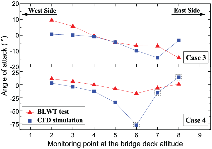
Angle of attack along the bridge deck (Type 3).

Envelope of wind speed ratio

Generally speaking, with the angle of attack changing, the wind speed ratio u/u_G would vary accordingly. Hence, if only the largest speed ratio were adopted in the mountain bridge designs, it would be unfavorable for the wind-resistant performances and less economical. Therefore, the wind speed ratio envelope varying with the angle of attack from the wind tunnel test is utilized to provide more references for the designs of the bridge, as displayed in Figure 13.

Figure 13.

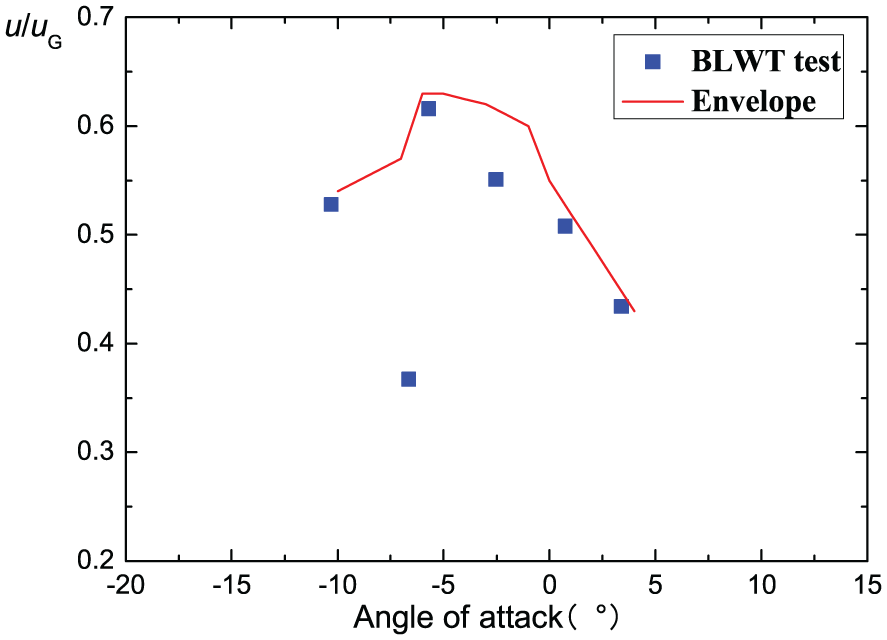
Wind speed envelope from BLWT test.

The envelope values from the two methods are listed in Table 1. CFD simulation results are 1.2 times larger than the BLWT test results at zero angle of attack. However, with the increase in angle of attack, the differences are narrowed and the values of two methods tend to be reasonably close to each other.

Table 1.

Envelopes of wind speed ratio u/u_G from BLWT test and CFD simulation.

Angle of attack (°)	−5	−7	−5	−3	−1	0	1	2	3	4
BLWT test	0.54	0.57	0.63	0.63	0.625	0.62	0.61	0.60	0.55	0.52
CFD simulation	0.45	0.60	0.75	0.75	0.75	0.75	0.75	0.75	0.62	0.55

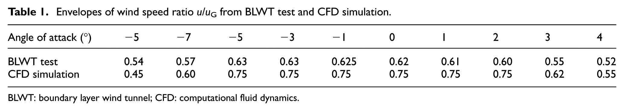
BLWT: boundary layer wind tunnel; CFD: computational fluid dynamics.

Turbulence intensities at the bridge site in the BLWT test

Turbulence intensity is an important parameter in the study of wind characteristics. Turbulence intensities were measured in the vertical direction at the mid-span of the bridge and along the bridge deck in the BLWT test. Due to the limitation of present grid in CFD simulation, it is hard to obtain the turbulence intensity. So the comparison on the turbulence intensity is not included in the article.

Profiles of longitudinal turbulence intensity I_u in the vertical direction are plotted in Figure 14. Turbulence intensity profiles of Type 1 are generally smaller than those of Type 2, for the terrain of Type 1 is less sheltered.

Figure 14.

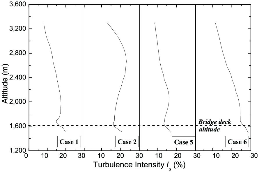
Turbulence intensity profiles in the vertical direction at the mid-span of the bridge.

As the turbulence intensity at the bridge deck altitude is more concerned in the wind-resistant designs of bridges, the variation of longitudinal turbulence intensity along the bridge deck is shown in Figure 15. Turbulence intensities of three eastern points are larger than other points for cases of the south wind (Cases 3–6), and large spatial variations are observed. As for Cases 1 and 2, turbulence intensities along the bridge deck remain unchangeable on the whole. It is supposed that larger turbulence intensities of the three eastern points for the south wind cases are caused by the flow separation due to southeastern ridge.

Figure 15.

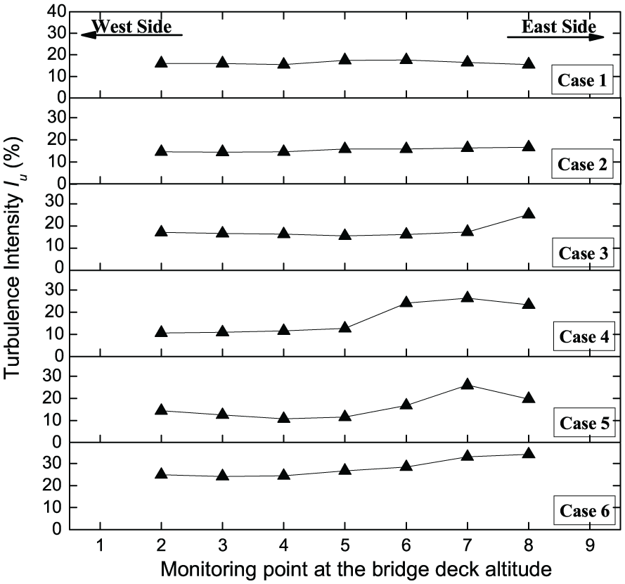
Turbulence intensity along the bridge deck.

Conclusion

To compare the wind characteristics obtained from the wind tunnel test and CFD simulation, studies on the wind characteristics at the typical bridge site in mountainous terrain were conducted. Some conclusions are drawn as follows:

For the open terrain, results from the two methods are reasonably close. For the open terrain with a steep slope close to the bridge, with the bridge located halfway up the gorge, high mountain shielding effects are obvious for both methods. However, the extents of the shielding effects appear different for the two methods, and the differences are mitigated with the increase in altitude.

Wind speed and angle of attack along the bridge deck are mainly influenced by the local terrain. Large spatial variations of wind speed are observed for south wind cases, and the results on the eastern side vary much more sharply in the CFD simulation. Since the wind speeds at the deck altitude are quite low for some cases in the CFD simulation, angles of attack are too large.

For the case of wind normal to top of the ridge, strong downslope wind is generated at the lee slope, which leads to negative angle of attack near the slope. However, for the case of wind flowing arising along the ridge, positive angle of attack is formed and mountain shielding effect is observed along the deck.

Envelopes of wind speed ratio are obtained for the two methods. With the increase in angle of attack, the differences are narrowed and the values from two methods tend to be reasonably close.

Turbulence intensities at the bridge site of Type 1 are generally less than those of Type 2 from the BLWT test. Large spatial variations of turbulence intensity are observed for the cases of south wind. The larger turbulence intensities of the three eastern points for the south wind cases are supposed to be caused by the flow separation due to the southeastern ridge.

Footnotes

Declaration of Conflicting Interests

The author(s) declared no potential conflicts of interest with respect to the research, authorship, and/or publication of this article.

Funding

The author(s) disclosed receipt of the following financial support for the research, authorship, and/or publication of this article: The authors are grateful for the supports of the National Natural Science Foundation of China (U1334201 and 90915006), the Construction Technology Project of China Transport Ministry (2014318800240), the Sichuan Province Youth Science and Technology Innovation Team (2015TD0004), and the Doctoral Innovation Funds of Southwest Jiaotong University.

References

Carpenter

Locke

(1999) Investigation of wind speeds over multiple two-dimensional hills. Journal of Wind Engineering and Industrial Aerodynamics 83(1–3): 109–120.

Chen

Hui

MCH

(2007) A comparative study of stationary and non-stationary wind models using field measurements. Boundary-Layer Meteorology 122(1): 105–121.

Davenport

King

JPC

(1990) The influence of topography on the dynamic wind loading of long span bridges. Journal of Wind Engineering and Industrial Aerodynamics 36: 1373–1382.

Derickson

Peterka

(2004) Development of a powerful hybrid tool for evaluating wind power in complex terrain: atmospheric numerical models and wind tunnels (AIAA Paper no. 2004–1005). In: 42nd AIAA Aerospace Sciences Meeting and Exhibit. Reno, NV, 5–8 January.

Huang

. (2015) The appropriate shape of the boundary transition section for a mountain-gorge terrain model in a wind tunnel test. Wind and Structures 20(1): 15–36.

Huang

(2013) Prediction of typhoon design wind speed and profile over complex terrain. Structural Engineering and Mechanics 45(1): 1–18.

JTG/T D60-01-2004 (2004) Wind-resistant Design Specification for Highway Bridges. Beijing, China: China Communication Press (in Chinese).

Chen

Zhang

. (2010) Wind tunnel modeling of flow over mountainous valley terrain. Wind and Structures 13(3): 275–292.

Cai

Tang

. (2011) Study of spatial distribution feature of wind fields over bridge site with a deep-cutting gorge using numerical simulation. China Civil Engineering Journal 44(2): 116–122 (in Chinese).

10.

Menter

(1994) Two-equation eddy-viscosity turbulence models for engineering applications. AIAA Journal 32(8): 1598–1605.

11.

Meroney

(1980) Wind-tunnel simulation of the flow over hills and complex terrain. Journal of Industrial Aerodynamics 5(3–4): 297–321.

12.

Neal

(1983) The influence of model scale on a wind-tunnel simulation of complex terrain. Journal of Wind Engineering and Industrial Aerodynamics 12(2): 125–143.

13.

Paterson

Holmes

(1993) Computation of wind flow over topography. Journal of Wind Engineering and Industrial Aerodynamics 46–47: 471–476.

14.

Sierputowski

Ostrowski

Cenedese

(1995) Experimental study of wind flow over the model of a valley. Journal of Wind Engineering and Industrial Aerodynamics 57(2–3): 127–136.

15.

Tamura

Iwatani

Hibi

. (2007) Profiles of mean wind speeds and vertical turbulence intensities measured at seashore and two inland sites using Doppler sodars. Journal of Wind Engineering and Industrial Aerodynamics 95(6): 411–427.

16.

Ucar

Balo

(2009) Investigation of wind characteristics and assessment of wind-generation potentiality in Uludağ-Bursa, Turkey. Applied Energy 86(3): 333–339.

17.

Uchida

Ohya

(1999) Numerical simulation of atmospheric flow over complex terrain. Journal of Wind Engineering and Industrial Aerodynamics 81(1–3): 283–293.

18.

Utsunomiya

Nagao

Yoshimura

(1989) Wind-tunnel and full-scale comparisons on the change of local wind characteristics due to an open cut. Journal of Wind Engineering and Industrial Aerodynamics 32(1–2): 51–61.

19.

Zhu

Wong

. (2000) Field measurement results of Tsing Ma suspension bridge during Typhoon Victor. Structural Engineering and Mechanics 10(6): 545–559.