
Abstract
In this article, the wavelet-Galerkin method is adopted for calculating structural dynamic responses under the framework of multiresolution analysis. At first, the second-order differential equation of motion is transformed into wavelet domain through function expansion with scaling function at the chosen resolution level. The number of basis function is uniquely determined, and the corresponding coefficients are approximated by numerical quadrature method. And then the two-term connection coefficients are derived and computed at various scales. After this, the dynamic responses of the system with single degree of freedom subjected to sinusoidal excitation are obtained and validated. Subsequently, the proposed method is extended to multidegree-of-freedom systems based on mode-superposition method. Finally, the parametric study is performed, and the simulation results show that the identified dynamic responses match the true responses very well with appropriate choice of the resolution level and the wavelet order.
Keywords
Introduction
In structural dynamics, the second-order differential equation of motion describes the behavior of structure (Cook, 2007). The dynamic responses are critical to assess structural safety and integrity. As a result, much effort has been devoted to seek the solution of equation of motion. In general, there are two basic categories: one is direct integration methods, where the dynamic response is achieved through step-by-step integration method in the time domain, such as Newmark-beta method (Craig and Kurdila, 2006), Wilson-theta method (Craig and Kurdila, 2006), and precise integration method (Wan-Xie, 2004). The other is indirect integration methods, where the equation of motion is converted into another domain, for example, frequency domain or wavelet domain (Hall and Beck, 1993; Humar and Xia, 1993; Venâncio Filho et al., 2002), in which dynamic responses are extracted. Herein, we focus on the indirect integration method.
For indirect integration methods, frequency-domain method was initially proposed and recognized as an effective and efficient method for calculating dynamic responses with the advent of fast Fourier transform (FFT) algorithm (Hall and Beck, 1993; Humar and Xia, 1993). However, the FFT-based methods have two main adverse problems to address: these methods are limited to cases with zero initial conditions and the hypotheses of periodic input result in a serious leakage problem particularly for short or non-stationary signals (Liu et al., 2015). In recent decades, wavelet transform and analysis have attracted substantial attention and gradually emerged as a powerful tool for signal processing (Chen et al., 2016) and numerical computation (Li and Chen, 2014). Wavelets are irregular, localized, and often non-symmetrical, which make them better describe abnormalities and transient phenomenon compared to harmonic functions. These properties guarantee wide applications of structural damage detection (Hester and González, 2012; Nguyen, 2015; Rucka and Wilde, 2006), feature extraction (Chandra and Sekhar, 2016), and system identification (Ghanem and Romeo, 2000; Xu et al., 2012). The heart of wavelet analysis is multiresolution analysis (MRA) which was presented by Mallat (1989). A function or signal can be decomposed into approximation and details by discrete wavelet transform (DWT). The approximation and details can be computed recursively with fast wavelet transform (FWT) at different levels of resolution under the framework of MRA. Daubechies (1988) constructed a family of wavelets characterized by compactly supported, orthogonality and exact representation of polynomials to a certain degree. On the context of MRA, Daubechies wavelets have been widely used for numerical computation. Amaratunga et al.(1994) presented wavelet-Galerkin method for one-dimensional partial differential equations, and they used the same procedure to handle boundary value problem (Amaratunga and Williams, 1997). Amaratunga and Williams (1995) provided a modified wavelet-Galerkin difference method for the first-order differential equation. Williams and Amaratunga (1997) proposed a wavelet extrapolation technique to eliminate the undesirable edge effects during the DWT of finite length data. Sattar et al. (2009) solved the water hammer equation with wavelet-Galerkin method. Tanaka et al. (2015) analyzed the dynamic stress concentration problems with wavelet-Galerkin method. Liu et al. (2011) proposed the multiscale wavelet-based method for two-dimensional (2D) elastic problems. Gopikrishna and Shrikhande (2011) presented a hierarchical finite element formulation for the solution of structural dynamic problems. Mahdavi and Razak (2015) used Haar wavelet and Chebyshev wavelet for the dynamic analysis of space structures. In the above methods, it is considered that a function or signal is represented by wavelets basis; however, few mentioned references refer to the number of basis function used, and the selection is usually subjective.
In this article, the wavelet-Galerkin method is used to solve the second-order differential equation of motion. First, the equation of motion is transformed into wavelet domain through function expansion. The number of basis function is determined uniquely, and the coefficient corresponding to basis function is approximated. And then, the two-term connection coefficients are derived and computed at various resolution levels. At the same time, the boundary problem and initial condition are handled carefully. The solution to the dynamic equation of motion is equivalent to seek for the solution of a set of linear algebra equations. Finally, the dynamic responses are reconstructed from the obtained coordinate coefficients. The proposed method is instructive in two aspects: the first is that one can view the dynamic response under the context of MRA and balance the solution accuracy and computation effort, and second, it is helpful to inverse problem solved in the wavelet domain (Ghanem and Romeo, 2000; Xu et al., 2012).
Wavelet-Galerkin method for structural dynamic analysis
The computation of structural dynamic responses
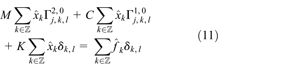
A linear time-invariant system with n-degree-of-freedom (DOF) systems subjected to external excitation can be described as

where
By introducing
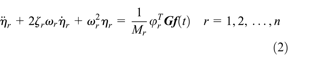
where
Wavelet-Galerkin method
The wavelet-Galerkin method is a projection method that seeks for an approximating solution through the projection of the exact solution onto a subspace spanned by wavelet basis. On the context of MRA, Daubechies wavelet family has wide application with the advantage of compactly supported, orthogonality and exact representation of polynomials to a certain degree. In this article, Daubechies wavelet is adopted. Herein, the wavelet-Galerkin solution for equation of motion is proposed and implemented. Consider a linear time-invariant dynamic system with single DOF subjected to external force formulated by

where M, C, and K are system mass, damping, and stiffness matrices, respectively;
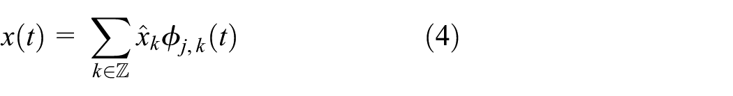
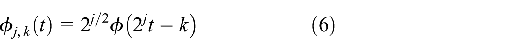
where j is the scale at which dynamic displacement is projected and k is translation parameter;
where
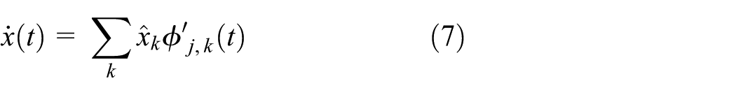
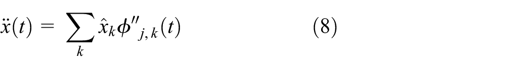
Then, the dynamic velocity and acceleration are formulated directly by
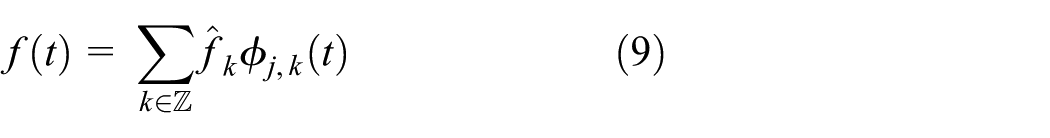
Similarly, the force is represented by
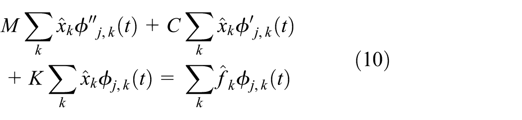
Then, equation (1) is rewritten as
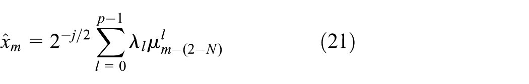
Both sides of equation (10) are multiplied by
where
Up to now, the dynamic equation is transformed into wavelet domain in equation (10). Before solving system dynamic responses with wavelet-Galerkin method, three crucial aspects should be carefully dealt with. First of all, the number of basis function
The computation of coordinate coefficients in the wavelet domain
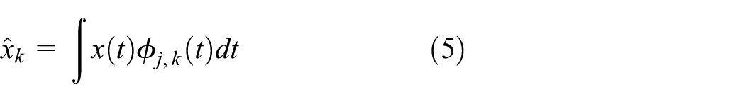
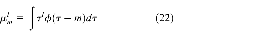
The dynamic response in the time domain can be represented in the wavelet domain spanned by a set of basis function

Because

Equation (15) must be calculated by quadrature methods since there are no explicit formulas for scaling function. Based on the fact that the coordinate coefficients of
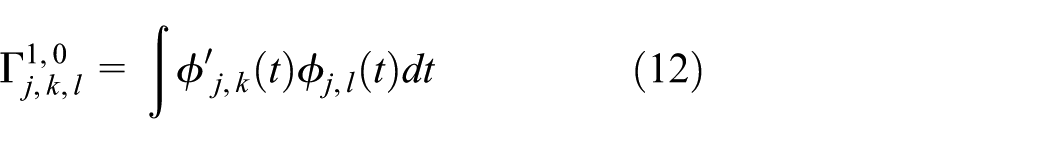
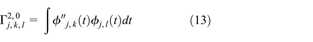
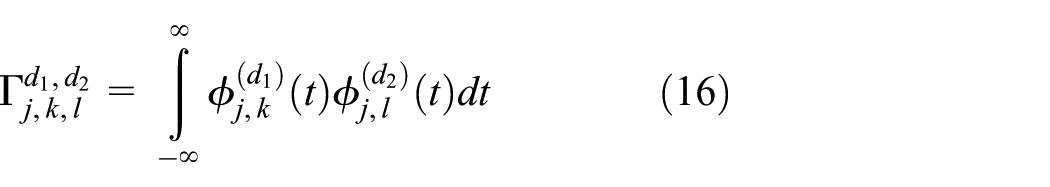
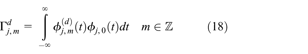
The computation of connection coefficients
In this article, only two-term connection coefficient is under discussion, which is defined generally as (Latto et al., 1991; Nielsen, 1998; Restrepo and Leaf, 1997)
where
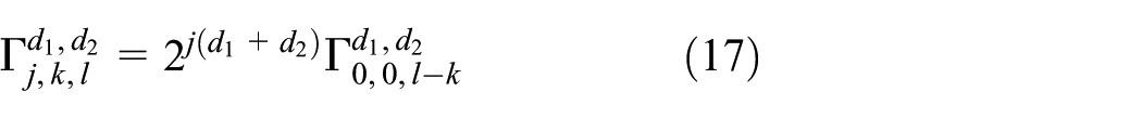
We have the identity
Using the changes in variable
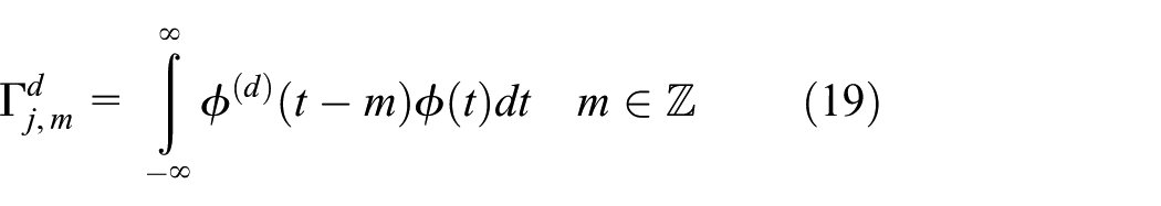
This is the same as the derivation of connection coefficients at scale
The boundary problem and initial condition
From equation (10), the connection coefficients
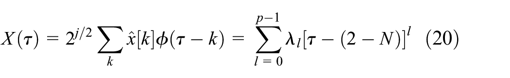
Both sides of equation (20) are multiplied by
where
It is suggested that the extrapolation parameter equals N (Williams and Amaratunga, 1997). Then, equation (21) can be written compactly in terms of
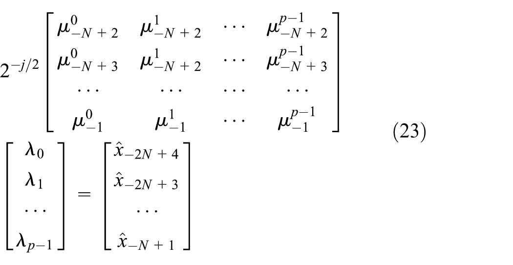
If it is assumed that the independent coordinate coefficients
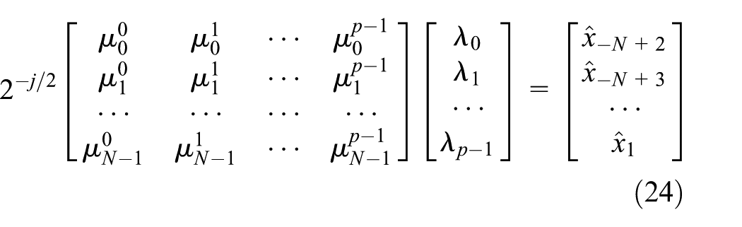
Based on equations (23) and (24), one can construct the transformation from the coordinates within the wavelet domain to the coordinates outside the wavelet domain at left boundary. The right boundary situation is handled in a similar way.
The initial condition for system dynamics must be considered. Suppose that
From equation (26), the first-order derivative of scaling function is required, which is calculated numerically based on Oslick et al. (1998).
In summary, the second-order differential equation in the time domain is converted into wavelet domain with a set of linear algebraic equations. The coordinate coefficients in the wavelet domain are solved by a combination of equations (10), (25), and (26). The dynamic responses are extracted from the obtained coordinate coefficients.
Case studies
In this section, several test cases will be tested, and the applicability of the proposed wavlet-Galerkin method for structural dynamic responses is validated. First, the displacement and velocity of the system with single DOF based on the wavelet-Galerkin method subjected to forced vibration are validated by comparing the results with true responses calculated based on Runge–Kutta algorithm in Simulink (Mathworks, 2015). Subsequently, the application of wavelet-Galerkin method for dynamic response is extended to system with multi-DOFs. And finally, the parametric study on dynamic responses are performed.
Single-DOF system
Consider a single-DOF system with zero initial condition subjected to external excitation given by

The following system parameters are under consideration:
where
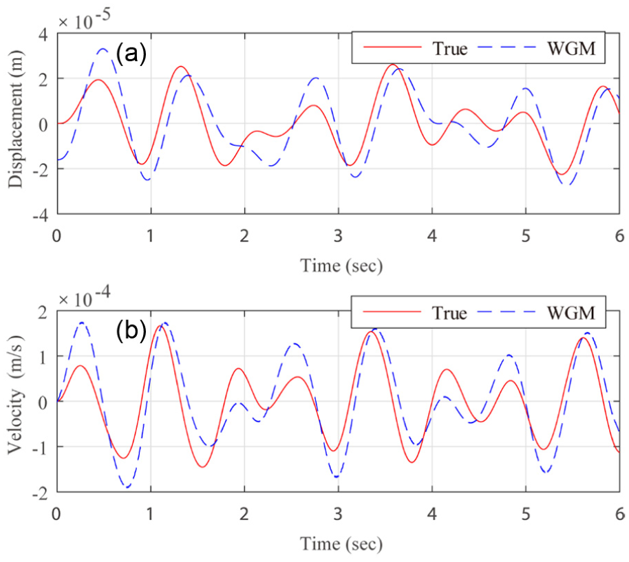
Dynamic responses with WGM (
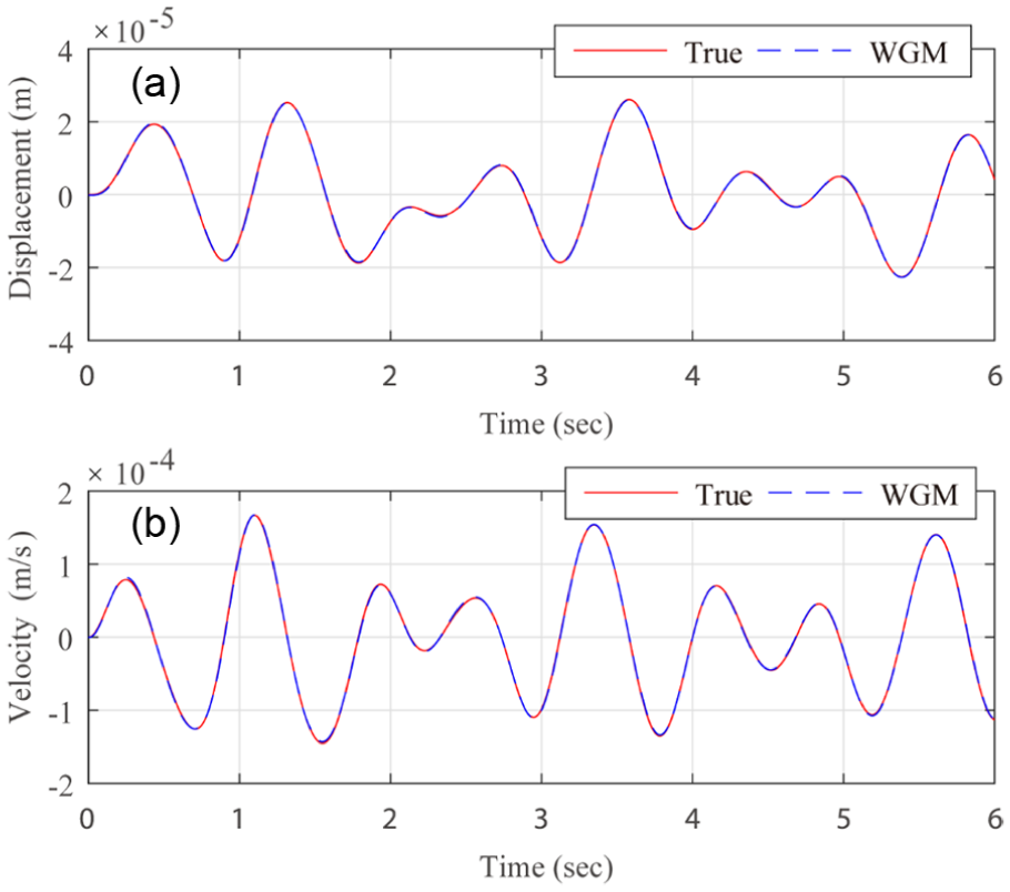
Dynamic responses with WGM (
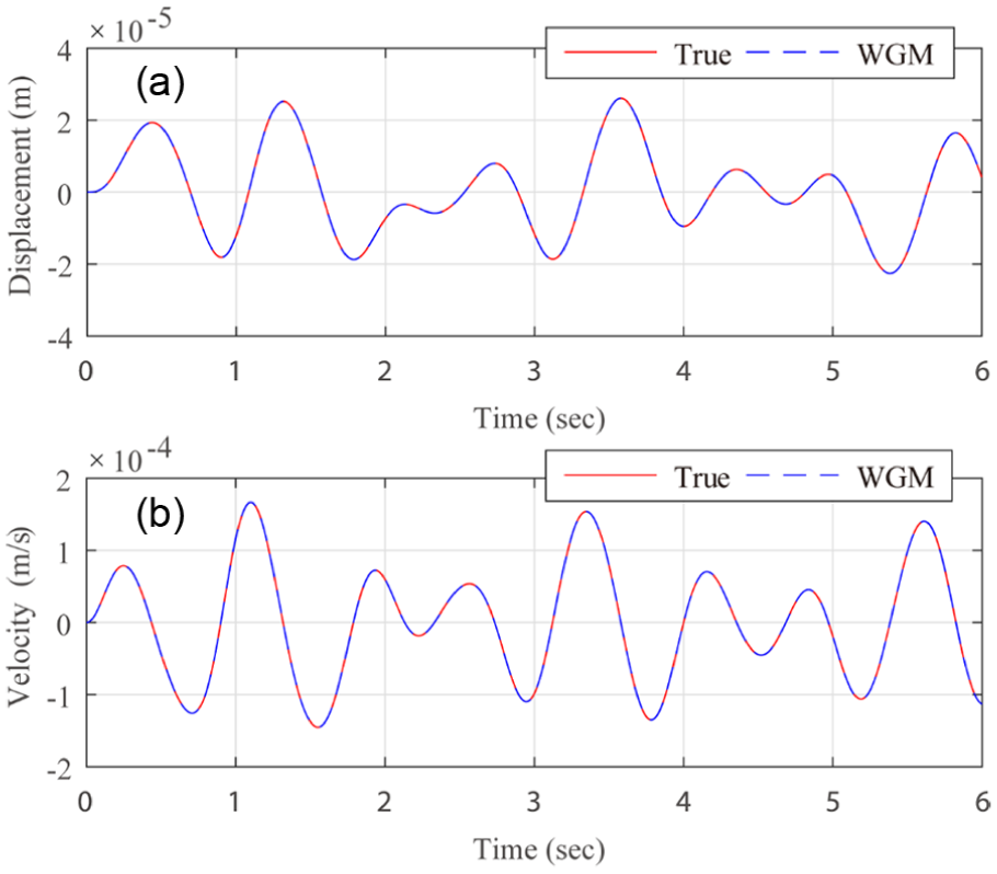
Dynamic responses with WGM (
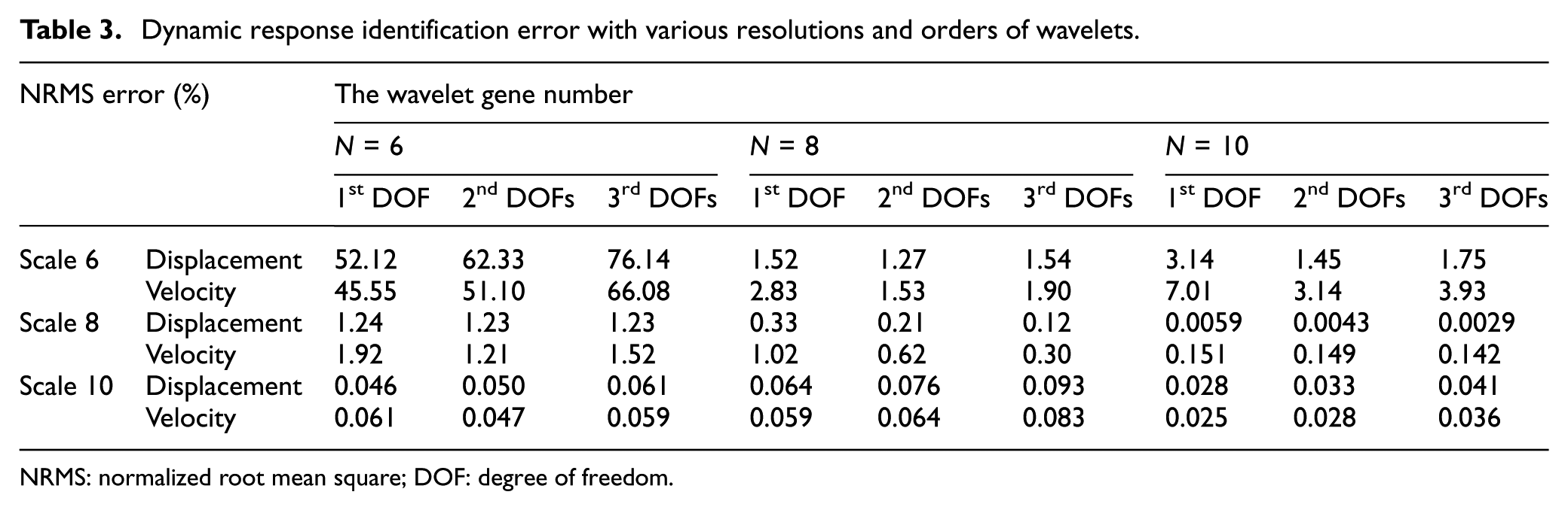
Dynamic response identification error with various resolutions and orders of wavelets.
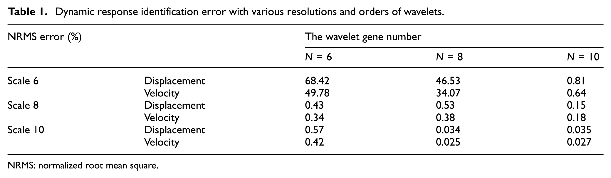
NRMS: normalized root mean square.
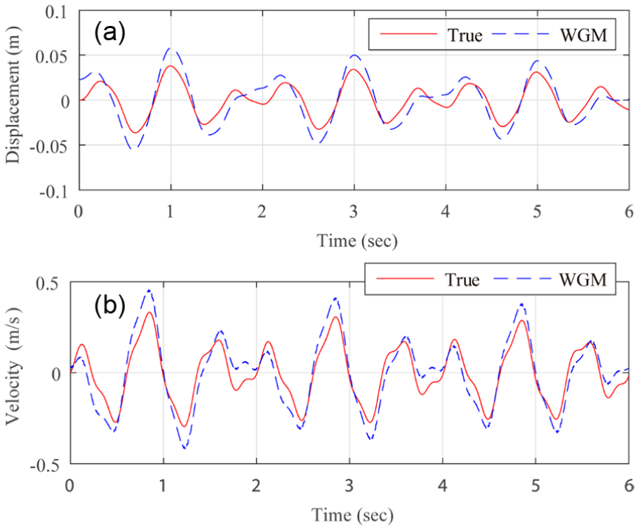
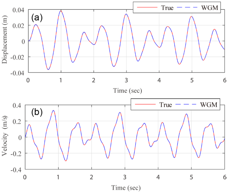
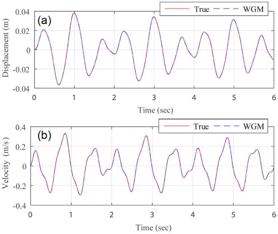
From Figure 1, the wavelet-Galerkin method failed to identify displacement and velocity at scale 6 with Db6. However, as the scale increased up to 8 and 10, the dynamic responses are calculated accurately with NRMS error of 0.43% and 0.57% for displacement and with NRMS error of 0.34% and 0.42% for velocity as shown in Figures 2 and 3, respectively. In Table 1, along the row direction, one can see that the identification performance improved as increased by the gene of wavelet. In column direction, the input reconstruction accuracy increased at higher resolution level. To be noted that when Db6 and Db8 are used, the dynamic responses cannot be extracted at scale 6 but match the true responses quite well when increased to the higher level resolution 10. This is maybe because the higher the order of wavelet, the smoother the shape of wavelet. For Db10, the dynamic responses are recovered successfully, and the identification accuracy improved as the resolution increased. In contrast to
In addition, noise effect is under investigation for dynamic response reconstruction. Three noise levels are considered. The white noise with 0%, 5%, and 10% NRMS noise-to-signal ratio is added to the exact input signal. For the sake of space, the dynamic response error for Db6 at various scales is under discussion, and the identification error is shown in Table 2. One can see that the wavelet-Galerkin method failed to extract the dynamic response at scale 6 under all noise levels. It is observed that the identification performance deteriorates as the noise level increased. However, at scale 8 or 10, the dynamic response identification error is under 4% NRMS even with 10% noise level.
Dynamic response identification error with noisy inputs for Db6.

NRMS: normalized root mean square.
Multi-DOF system
The procedure of seeking dynamic responses of the system with single DOF is extended to the multi-DOF cases. Consider a shear building model with 3 DOFs as shown in Figure 4, where
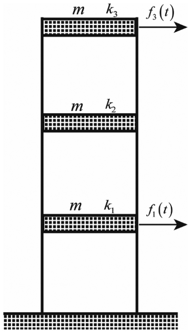
Shear building model with 3 DOFs.
Dynamic responses with WGM (
Dynamic responses with WGM (
Dynamic responses with WGM (
Dynamic response identification error with various resolutions and orders of wavelets.
NRMS: normalized root mean square; DOF: degree of freedom.
In order to evaluate the robustness of the proposed method to noise, similar to the single-DOF case, the three same noise levels are considered for multi-DOF system, and the identification error for Db6 is only discussed. The results are summarized in Table 4. One can see that the wavelet-Galerkin method failed to extract the dynamic response at scale 6 under all noise levels. It is observed that the identification performance deteriorates much slowly as the noise level increased. However, at scale 8 or 10, the dynamic response identification error is under the order of 5% NRMS even with 10% noise level. It is validated that the presented method is robust to noise effect.
Dynamic response identification error with noisy inputs for Db6.
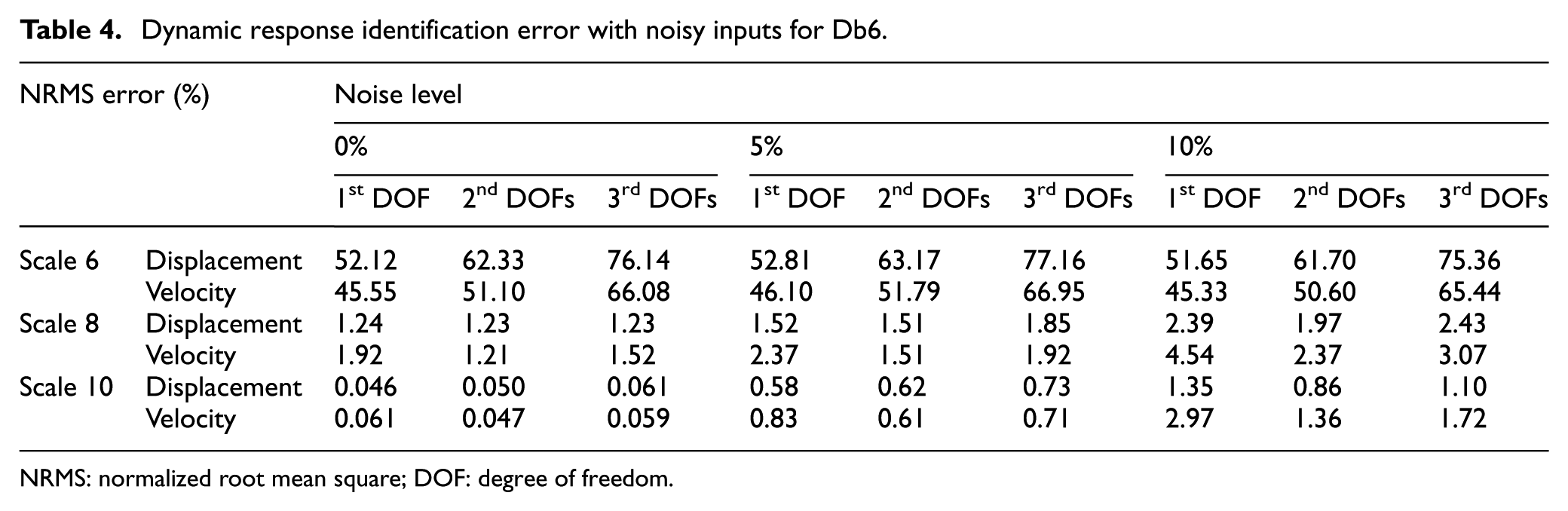
NRMS: normalized root mean square; DOF: degree of freedom.
Summaries and conclusion
In this article, the wavelet-Galerkin method with the advantage of Daubechies wavelet is adopted to compute the dynamic responses of the second-order differential equation of motion. The number of basis function is derived analytically, and the corresponding coefficients are approximated by numerical quadrature method. And then the two-term connection coefficients are derived and computed at various scales. The proposed method is tested and validated from single-DOF system to multi-DOF system. In addition, the parametric study is conducted. The conclusions drawn from theoretical derivation and numerical studies are summarized as follows:
The proposed wavelet-Galerkin method for dynamic response is tested and validated for single-DOF and multi-DOF systems. The dynamic response can be recovered accurately with right choice of scale and wavelet order.
The wavelet-Galerkin method is robust to noise effect. From numerical results, the dynamic response reconstruction errors are under 2% NRMS error without noise and 5% NRMS error under 10% noise level when decomposed at scale 8 or 10.
From the numerical studies of single or multiple systems, it is observed that generally the higher the resolution level and wavelet order, the higher the accuracy of displacement and velocity.
The dynamic response is calculated by the wavelet-Galerkin method under the framework of MRA. The higher the scale at which the signal is decomposed, the larger the sampling points are used, and the more the computation time is needed. One can balance the identification accuracy and computation effort.
Footnotes
Appendix 1
Declaration of Conflicting Interests
The author(s) declared no potential conflicts of interest with respect to the research, authorship, and/or publication of this article.
Funding
The author(s) disclosed receipt of the following financial support for the research, authorship, and/or publication of this article: This research work was jointly supported by the 973 Program (2015CB060000), the National Natural Science Foundation of China (51625802, 51478081), the Science Fund for Distinguished Young Scholars of Dalian (2015J12JH209), and the Fundamental Research Funds for the Central Universities (DUT16LAB07).