Nonlinear joint model updating of strong column-weak beam type frames based on instantaneous characteristics of the responses under earthquake excitations

Abstract

In this article, a novel method based on the instantaneous frequencies and amplitudes of the principal response components is presented for nonlinear joint model updating. The instantaneous frequencies and amplitudes are first extracted by a low-pass filter with Hilbert transform. Then, limited point values of the extracted instantaneous frequencies and amplitudes are applied to represent the response of the nonlinear structure. Finally, an objective function based on the residuals of instantaneous frequencies and amplitudes between experimental structure and finite element model is established using the response surface method. The optimal values of the nonlinear joint model parameters are obtained by minimizing the objective function using simulated annealing algorithm. To verify the effectiveness of the proposed method, a three-story frame with bilinear moment–rotation relationship at the beam-column joints under earthquake excitations is simulated as a numerical example. The accuracy of the proposed nonlinear joint model updating procedure is quantified using the defined error indices. The effects of the selected data point number and the weight factors in the objective function are also discussed in the article. The results indicate that the proposed method can effectively update the nonlinear joint model with high accuracy even with noise effect.

Keywords

Hilbert transform instantaneous amplitude instantaneous frequency nonlinear joint model updating response surface method

Introduction

Over the past decades, finite element (FE) model updating that modifies the model parameters based on the experimental results to achieve a more realistic model (Friswell and Mottershead, 1995) has received increased attention in structural dynamics. Overall, FE model updating can be mainly divided into two types: matrix type and parameter type. The matrix type methods are one-step non-iterative procedures that directly update the elements of stiffness and/or mass matrices (Baruch and Bar Itzhack, 1978; Berman and Nagy, 1983). However, these methods come into the problem that the updated matrices are not always physically meaningful (Jaishi and Ren, 2005). Therefore, the parameter type methods provide a new way for FE model updating. These methods construct an objective function based on the residuals of structural response features between analytical and experimental results, and the model parameters are then updated by minimizing the objective function with different optimization algorithms. For instance, Link (1999) gave an overview of the sensitivity-based updating methods in structural dynamics. Jaishi and Ren (2005, 2007) used either single-objective or multi-objective optimization technique to update the FE models of civil engineering structures. However, these sensitivity-based methods may cause not only considerable computational intensive but also convergence difficulty especially when the real structure is complex.

To overcome the complex structural model issue, the response surface (RS) methodology (Box and Wilson, 1951) is introduced for FE model updating. With the design of experiments, the original FE model can be replaced by the RS model maintaining high accuracy for optimization purposes. For instance, Guo and Zhang (2004) applied the RS models with central composite design to update an H-shaped structure and found that the RS-based model updating method which can obtain almost the same accurate results is much more cost-efficient than the traditional sensitivity-based model updating method. Ren et al. (2010) further applied RS model to FE model updating using either structural dynamic or static responses. It was concluded that the RS method is more efficient and converges faster compared with the traditional sensitivity-based model updating method especially when the structure is complex and the number of model parameters is large.

However, complex nonlinear behavior of structures has been observed not only when they are subjected to extreme loads (such as earthquake and typhoon) but also during the operational conditions. Characterization of the nonlinearity may provide critical diagnostic and prognostic information. Thus, it is critical to know if a structure is behaving nonlinearly and to detect and estimate the impact of the nonlinearity. Hasselman et al. (1998) applied the principal component analysis for nonlinear model correlation, updating, and uncertainty evaluation. Lenaerts et al. (2001) investigated the use of the proper orthogonal decomposition for model updating of nonlinear mechanical systems. Hemez and Doebling (2001) presented a clear review and assessment of model updating for nonlinear transient dynamics. They discussed the current challenges in inverse problem solving and addressed the correlation of nonlinear models with test data. Zhang and Guo (2007) applied the design of experiment and principal component decomposition to extract nonlinear dynamic feature for updating and validation of a frame structure with nonlinear thin-walled component. Silva et al. (2009) presented a detailed comparative study of nonlinear model updating approaches, such as harmonic balance method, constitutive equation error, restoring force surface, and proper orthogonal decomposition. Song et al. (2009) further updated a nonlinear FE model of a reinforced concrete structure under low excitation. Recently, the second-order orthogonal Wiener kernel was introduced to update nonlinear structures (Silva, 2011). Shahidi and Pakzad (2013) further presented a procedure based on RS to update nonlinear FE models in the time domain. More recently, Asgarieh et al. (2014) proposed a novel method for nonlinear FE model updating of a frame with Bouc–Wen hysteresis model based on the time-varying modal parameters (which were estimated using the deterministic–stochastic subspace identification method). Both numerical and experimental applications showed the effectiveness and high accuracy of this method. Wang et al. (2015) established a new objective function based on the instantaneous frequencies and amplitudes for nonlinear structural model updating.

Since the nonlinear behaviors of structures are mainly caused by local nonlinearities (such as gaps, friction, and joints), researchers further studied local nonlinear model updating. Through matching simulated and measured data, Schmidt (1994) discussed FE model updating with local nonlinearities. Meyer and Link (2003) applied harmonic balance method to identify local nonlinear stiffness and damping parameters to obtain a reasonable description in the frequency domain. Iranzad and Ahmadian (2012) updated a bolted joint which was modeled by a thin layer with elastic–plastic material. Davoodi et al. (2012) determined the nonlinear behavior of a ball joint system using static deflections and genetic algorithm. Alamdari et al. (2013) adopted Richard–Abbot elastic–plastic material to describe the nonlinear joint interface, and the four material parameters were used for model updating based on structural frequency response function. Lei et al. (2014) presented a two-step Kalman filter approach for the damage detection of frame structures with joint damage under earthquake excitation using partial measurements of structural acceleration responses.

For many structures, the nonlinear behavior of the structure under extreme loads can be described by the nonlinear hysteresis loops. The area of a hysteresis loop equals the energy dissipation in a cycle. Both typical nonlinear stiffness and nonlinear damping systems can be included in the hysteresis systems. Therefore, in order to update the nonlinear model, it is suggested to update the hysteresis parameters of nonlinear structures, whose nonlinearities are simulated by defining hysteresis models. For instance, Ebrahimian et al. (2015) combined the advanced mechanics-based nonlinear structural FE models and the maximum likelihood estimation method to estimate time-invariant parameters of the nonlinear hysteretic material constitutive models. With excitation decomposition algorithm, Ding et al. (2015) proposed an improved unscented Kalman filter to identify the structural parameters and coefficients of the orthogonal decomposition. Based on these studies, the overall process of nonlinear model updating may include (1) using suitable nonlinear hysteresis model to simulate the actual structure, (2) establishing objective function according to nonlinear characteristics, and (3) minimizing objective function with optimization algorithm to update nonlinear hysteresis parameters.

In this article, a new nonlinear joint model updating method for strong column-weak beam type frame structures with hysteresis models is proposed based on the instantaneous characteristics of the principal response components. Since the nonlinear response is combined with several mono-components with time-varying frequency and amplitude, and the original principal components can be reconstructed by the instantaneous frequency and amplitude, these two instantaneous parameters are used for objective function creation. Combining the analytical mode decomposition (AMD) proposed by Chen and Wang (2012), Wang et al. (2013), and Wang and Chen (2013) and Hilbert transform, the instantaneous frequencies and amplitudes of the principal response components are first extracted. Then, limited point values of the extracted instantaneous frequencies and amplitudes are selected for model updating. Finally, the objective function based on the residuals of instantaneous frequencies and amplitudes between experimental structure and FE model is established using the RS method. The objective function is then minimized using simulated annealing algorithm (Dekkers and Aarts, 1991; Kirkpatrick, 1984), and the optimal values of the nonlinear joint model parameters are obtained. To validate the effectiveness of the proposed method, a three-story frame with bilinear moment–rotation relationship at the beam-column joints under an earthquake is simulated as a numerical example. The accuracy of the proposed nonlinear model updating procedure is quantified using the defined error indices. The effects of the selected data point number and the weight factors in the objective function are also studied in the article.

Theoretical background

Instantaneous characteristics extraction

The nonlinear characteristics of a nonlinear structure are implied in the responses during the oscillation. However, it is difficult to directly use the responses to create an objective function for nonlinear structural model updating. Since the response of a nonlinear structure is combined with several mono-components, which can be reconstructed by their instantaneous frequencies and amplitudes, therefore, the instantaneous frequencies and amplitudes of the principal response components can be selected to represent the nonlinear characteristics of the structure.

To conduct the nonlinear joint model updating, the principal components are first extracted from the nonlinear vibration response by AMD. Then, the characteristics such as instantaneous frequencies and amplitudes of the principal components are obtained by constructing analytical signal with Hilbert transform. The analytical signal $z_{i} (t)$ of each component $x_{i} (t)$ is expressed as

z_{i} (t) = x_{i} (t) + H [x_{i} (t)] = A_{i} (t) e^{j \int ω_{i} (t) d t}

(1)

Since the instantaneous frequency and the amplitudes of the acceleration and displacement both slowly vary with time, thus, in this article, the instantaneous amplitude $A_{i} (t)$ and the slow-varying portion of $ω_{i} (t)$ of the decomposed mono-component are used to create objective functions for nonlinear model updating.

RS methodology

The traditional model updating methods have several drawbacks such as requirement of sensitivity calculations and cannot be used for nonlinear FE model updating (Zhang and Guo, 2007). Thus, in this article, the RS methodology is introduced to achieve the global approximations of the structural responses.

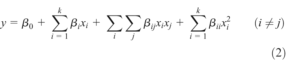
One of the important steps involved in RS-based method is the choice of RS form to express structural response features, which may have a great impact on the results of the analysis. The choice of RS models may depend on the type of application. For the FE model updating in structural dynamics, since polynomial model has shown attractive potential due to its simple calculation and closed-form algebraic type (Ren and Chen, 2010), a quadratic polynomial RS is used as

y = β_{0} + \sum_{i = 1}^{k} β_{i} x_{i} + \sum_{i} \sum_{j} β_{i j} x_{i} x_{j} + \sum_{i = 1}^{k} β_{i i} x_{i}^{2} (i \neq j)

(2)

where $y$ is response data, and $β_{0}$ , $β_{i}$ , $β_{i i}$ , and $β_{i j}$ are the regression coefficients to be estimated from the experimental data.

In order to economize computational efforts, the uniform design proposed by Fang (1980) and Wang and Fang (1981) to effectively solve the experimental problems with multiple parameters and levels is used to construct the RS models for the replacement of the original FE model. Several points are sampled in the RS domain based on the number of factors and the uniform design tables. Then, all the responses of design points are computed by FE analysis and corresponding instantaneous characteristics are extracted for constructing RS models with least-square estimation techniques. To update the nonlinear structural model through time history of the measured responses, a polynomial RS model is constructed to represent the results of FE model at every selected data point along the time series.

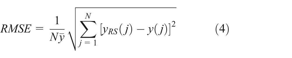
In this article, the accuracy of the regressed surface at every selected data point is verified based on the residuals of the RS and FE models. The overall adequacy of the RS models is evaluated by the R² criterion and root mean squared error (RMSE) criterion

R^{2} = 1 - \frac{\sum_{j = 1}^{N} {[y_{R S} (j) - y (j)]}^{2}}{\sum_{j = 1}^{N} {[y (j) - \bar{y}]}^{2}}

(3)

R M S E = \frac{1}{N \bar{y}} \sqrt{\sum_{j = 1}^{N} {[y_{R S} (j) - y (j)]}^{2}}

(4)

where $y_{R S}$ is the response value of the confirmation samples, $y$ is the true value of the confirmation samples, and $\bar{y}$ is the mean of all true values. The larger the value of $R^{2}$ , the more accurate the regressed RS. On the contrary, the smaller the value of $R M S E$ , the closer the fit to the data.

Parameter optimization

As discussed in section “Instantaneous characteristics extraction,” the slow-varying portion of the instantaneous frequency $ω (t)$ of the acceleration, acceleration amplitude $A_{a c c} (t)$ , and displacement amplitude $A_{d i s p} (t)$ are used for nonlinear model updating. The bilinear moment–rotation relationship is used to simulate the local nonlinearities at the beam-column joints in order to reflect the strong column-weak beam. The bilinear hysteresis parameters can then be updated by minimizing the residuals between analytical and measured instantaneous frequencies and amplitudes of the responses. An optimization objective function $J (θ)$ is defined as a sum of instantaneous residuals at selected time points along the response time series, which can be denoted as

J (θ) = \frac{1}{N_{m}} [J_{ω} (θ) + J_{a c c} (θ) + J_{d i s p} (θ)]

(5)

J_{ω} (θ) = \sum_{i = 1}^{N_{m}} \sum_{j = 1}^{N_{t}} \frac{1}{N_{t}} {[\frac{ω_{j}^{i} (θ, t) - {\hat{ω}}_{j}^{i} (t)}{{\hat{ω}}_{j}^{i} (t)}]}^{2}

(6)

J_{a c c} (θ) = \sum_{i = 1}^{N_{m}} \sum_{j = 1}^{N_{t}} \frac{1}{N_{t}} {[\frac{A_{a c c, j}^{i} (θ, t) - {\hat{A}}_{a c c, j}^{i} (t)}{{\hat{A}}_{a c c, j}^{i} (t)}]}^{2}

(7)

J_{d i s p} (θ) = \sum_{i = 1}^{N_{m}} \sum_{j = 1}^{N_{t}} \frac{1}{N_{t}} {[\frac{A_{d i s p, j}^{i} (θ, t) - {\hat{A}}_{d i s p, j}^{i} (t)}{{\hat{A}}_{d i s p, j}^{i} (t)}]}^{2}

(8)

in which $θ$ is the vector of the updating parameters. With equal weight factors, $J_{ω} (θ)$ , $J_{a c c} (θ)$ , and $J_{d i s p} (θ)$ are the residuals of frequency, acceleration, and displacement, respectively. $ω_{j}^{i} (θ, t)$ and ${\hat{ω}}_{j}^{i} (t)$ are the model predicted and experimentally identified instantaneous frequency of the ith mono-component at time j, respectively. $A_{a c c, j}^{i} (θ, t)$ and ${\hat{A}}_{a c c, j}^{i} (t)$ are the model predicted and experimentally identified instantaneous acceleration amplitudes of the ith mono-component at time j, respectively. $A_{d i s p, j}^{i} (θ, t)$ and ${\hat{A}}_{d i s p, j}^{i} (t)$ are the model predicted and experimentally identified instantaneous displacement amplitudes of the ith mono-component at time j, respectively. $N_{m}$ and $N_{t}$ are the number of mono-components and the selected measured time points, respectively.

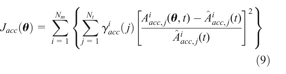
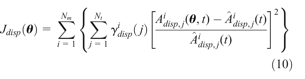
To consider the significance of maximum displacement and acceleration responses from the design point of view, the residuals of acceleration and displacement responses with unequal weight factors are defined and added into the objective function as follows

J_{a c c} (θ) = \sum_{i = 1}^{N_{m}} {\sum_{j = 1}^{N_{t}} γ_{a c c}^{i} (j) {[\frac{A_{a c c, j}^{i} (θ, t) - {\hat{A}}_{a c c, j}^{i} (t)}{{\hat{A}}_{a c c, j}^{i} (t)}]}^{2}}

(9)

J_{d i s p} (θ) = \sum_{i = 1}^{N_{m}} {\sum_{j = 1}^{N_{t}} γ_{d i s p}^{i} (j) {[\frac{A_{d i s p, j}^{i} (θ, t) - {\hat{A}}_{d i s p, j}^{i} (t)}{{\hat{A}}_{d i s p, j}^{i} (t)}]}^{2}}

(10)

γ_{a c c}^{i} (j) = \frac{\frac{{\hat{A}}_{a c c, j}^{i} (t)}{{\hat{A}}_{a c c, \max}^{i}}}{\sum_{j = 1}^{N_{t}} \frac{{\hat{A}}_{a c c, j}^{i} (t)}{{\hat{A}}_{a c c, \max}^{i}}}, γ_{d i s p}^{i} (j) = \frac{\frac{{\hat{A}}_{d i s p, j}^{i} (t)}{{\hat{A}}_{d i s p, \max}^{i}}}{\sum_{j = 1}^{N_{t}} \frac{{\hat{A}}_{d i s p, j}^{i} (t)}{{\hat{A}}_{d i s p, \max}^{i}}}

(11)

where $γ_{a c c}^{i} (j)$ and $γ_{d i s p}^{i} (j)$ are the defined weight factors of acceleration and displacement responses, respectively.

After parameterized, the nonlinear model updating problem turns into an optimization problem of structural parameters. In this article, the simulated annealing global optimization algorithm in MATLAB is used for minimizing the objective function $J (θ)$ , and the parameters vector $θ$ can then be obtained. The accuracy of updated results is evaluated using three different error indices, namely, frequency error $E_{w}$ , acceleration error $E_{a c c}$ , and displacement error $E_{d i s p}$ between real model and updated model. These error indices are defined as

E_{w} = \frac{{‖ ω_{u p d a t e d} - ω_{r e a l} ‖}_{2}}{{‖ ω_{r e a l} ‖}_{2}} \times 100 %

(12)

E_{a c c} = \frac{{‖ A c c_{u p d a t e d} - A c c_{r e a l} ‖}_{2}}{{‖ A c c_{r e a l} ‖}_{2}} \times 100 %

(13)

E_{d i s p} = \frac{{‖ D i s p_{u p d a t e d} - D i s p_{r e a l} ‖}_{2}}{{‖ D i s p_{r e a l} ‖}_{2}} \times 100 %

(14)

in which, $ω_{u p d a t e d}$ and $ω_{r e a l}$ are the instantaneous frequency’s slow-varying portion of the updated model and real model, respectively. $A c c_{u p d a t e d}$ and $A c c_{r e a l}$ are the acceleration of the updated model and real model, respectively. $D i s p_{u p d a t e d}$ and $D i s p_{r e a l}$ are the displacement of the updated model and real model, respectively. $‖ \dots ‖_{2}$ represents 2-norm value.

During the updating process, different stages involved in the method are gone through by the use of the prepared program. The overall steps of the nonlinear joint model updating process are shown in Figure 1.

Figure 1.

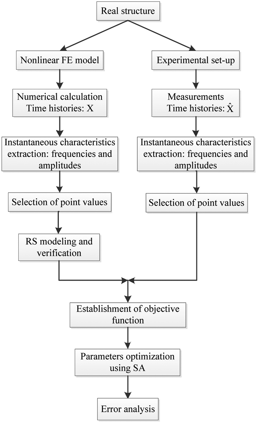
Overall stages of the nonlinear joint model updating process.

Numerical verification

Model description and dynamic analysis

In order to verify the feasibility of the method described above, a strong column-weak beam type two-dimensional three-story nonlinear frame is simulated. The bilinear moment–rotation relationship is used to simulate the local nonlinearities. The structure illustrated in Figure 2 is composed of beams and columns with cross-section dimensions of 0.25 m × 0.3 mand 0.3 m × 0.3 m, respectively. The span is 6 m and the total height is 12 m. The bottom ends of the columns are fixed. The nonlinear model is simulated using the FE analysis software ANSYS (DeSalvo and Swanson, 1989). Beam3 element is used to simulate the beams and columns, while Combin40 element is introduced to simulate the bilinear moment–rotation relationship at the beam-column joints. Material model behavior of beams and columns is elastic, and Young’s modulus, density, and Poisson’s ratio are 30 GPa, 2500 kg/m³, and 0.3, respectively. Initial values of bilinear hysteretic parameters are selected as: stiffness before yielding K₁ = 6.867 × 10⁶ kN m, stiffness after yielding K₂ = 8.134 × 10⁴ kN m, and yielding rotation X = 3.406 mrad.

Figure 2.

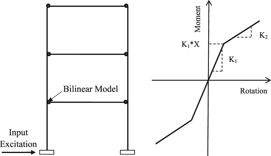
Three-story nonlinear finite element model and bilinear model.

In the study, the El-Centro earthquake shown in Figure 3 is selected as an external excitation and the structural damping ratio is assigned as 5%. The simulated acceleration and displacement responses with a sampling frequency of 200 Hz at the second floor are assumed as measured responses (Figure 4). The Fourier spectra of the acceleration response and the nonlinear moment–rotation loops are illustrated in Figure 5(a) and (b), respectively.

Figure 3.

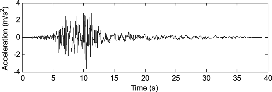
Acceleration record of El-Centro earthquake.

Figure 4.

Acceleration response of the second floor.

Figure 5.

(a) The Fourier spectrum of the measured acceleration and (b) the nonlinear moment–rotation hysteretic loops.

Nonlinear joint model updating

In this section, the three parameters of the bilinear moment–rotation relationship at the beam-column joints are selected as model parameters to be updated. Based on the previous studies and experiences, 20% is set to the parameter bounds. The uniform design method in design of experiments is then used to determine the sampling points. A total of 25 runs of experiments are carried out. Dynamic responses of different parameter levels under El-Centro earthquake are calculated, and the time history response data of the node at the middle of the second floor are used to extract the instantaneous frequencies and amplitudes of the principal components combined with AMD and Hilbert transform.

Since the slow-varying portion of the instantaneous frequency and the instantaneous amplitudes of the nonlinear structural responses vary slowly over time compared with the oscillation of the acceleration and displacement, there is no need to select all the measured time points to calculate instantaneous parameter residuals included in the objective function. The objective function can be created using limited point values along the time series of the response and a reasonable estimated result may be obtained. However, the selection of point values and the number of data points required are the critical issues that should be focused on when creating the objective function. So, in order to discuss the effect of selected data points, total five cases are considered here for this special example:

Case 1: 10 data points are equally selected from the response time series.

Case 2: 15 data points are equally selected from the response time series.

Case 3: 20 data points are equally selected from the response time series.

Case 4: 25 data points are equally selected from the response time series.

Case 5: In this case, considering the importance of local maximum, the time series of the instantaneous characteristics are equally divided into 20 intervals. Then, the location of the peak value in each interval is selected as the selected data point location.

The 20 selected local peak values of acceleration amplitude, displacement amplitude, and the instantaneous frequency of the measured (original) responses (Case 5) are presented in Figure 6(a) to (c).

Figure 6.

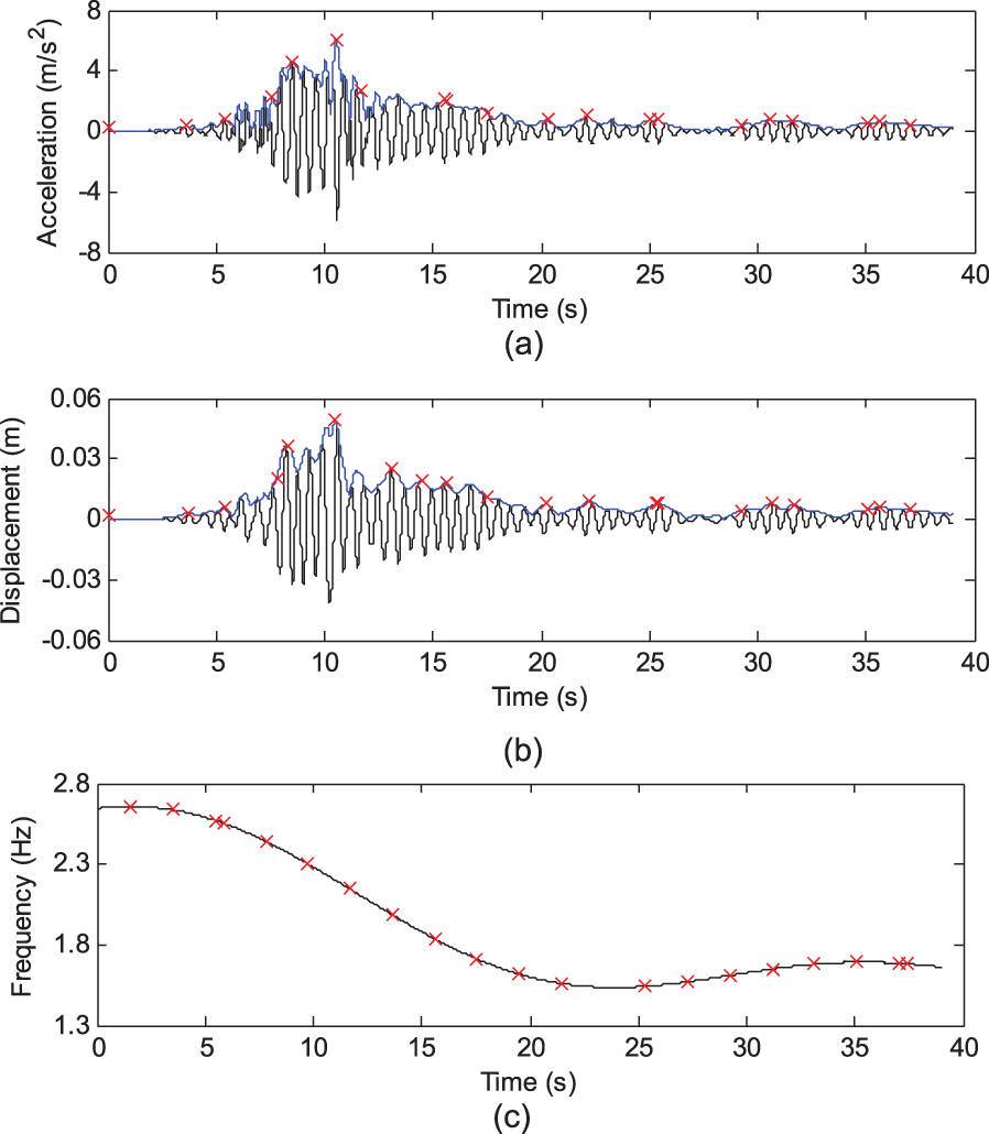
Selected data points of the dominant mono-component: (a) instantaneous amplitude of the acceleration, (b) instantaneous amplitude of the displacement, and (c) instantaneous frequency of the acceleration (Case 5).

After selecting the data points of instantaneous characteristics, a RS model is constructed at every selected data point to replace the FE model. To check the accuracy of the regressed surface, the $R^{2}$ and $R M S E$ are calculated for each data point of Case 1 to Case 5. As shown in Table 1, it is demonstrated that all $R^{2}$ values are close to 1, while all $R M S E$ values are close to 0, which indicates that every created RS has high regression accuracy.

Table 1.

The $R^{2}$ and $R M S E$ values of each RS model.

	Frequency	Acceleration amplitude	Displacement amplitude
$R^{2}$	0.9856–0.9922	0.9919–0.9996	0.9867–0.9981
$R M S E$	0.0018–0.0033	0.0011–0.0029	0.0013–0.0035

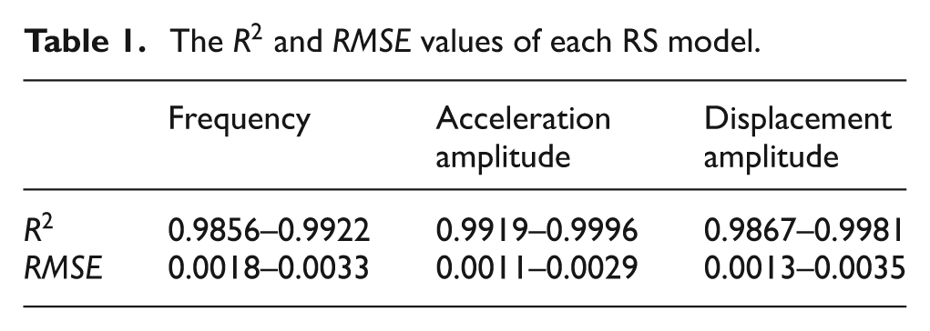
Then, the FE model is replaced by the regressed quadratic polynomial and the corresponding objective function is created for the nonlinear joint model updating. The hysteresis parameters are finally obtained by minimizing the objective function using simulated annealing algorithm.

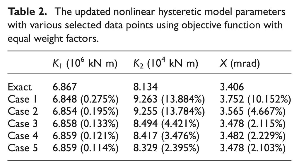
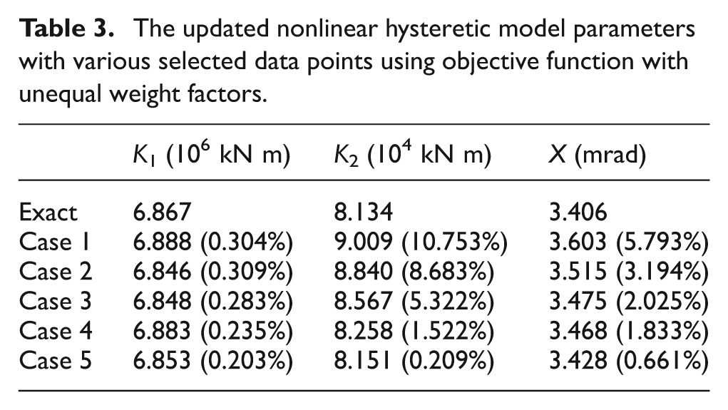
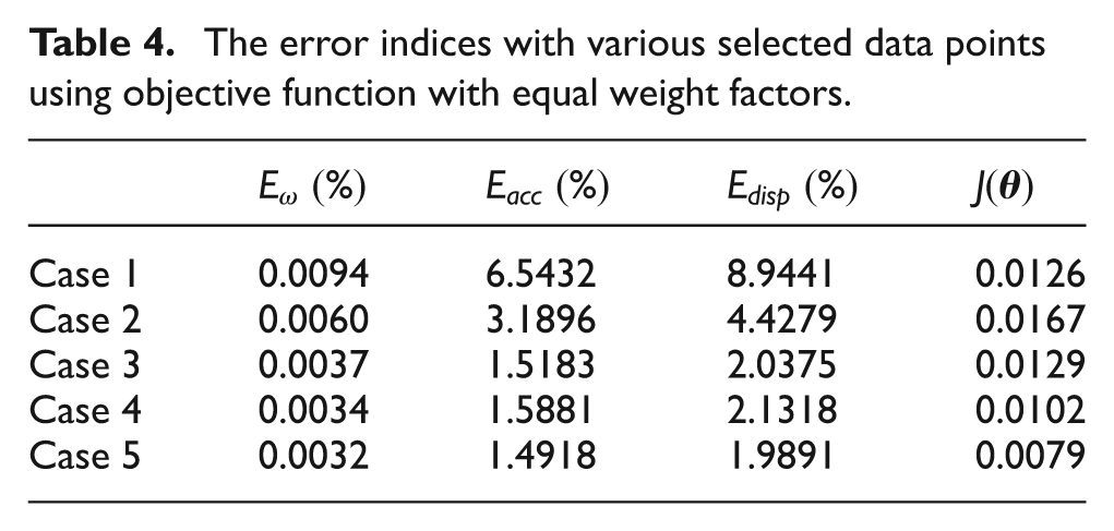
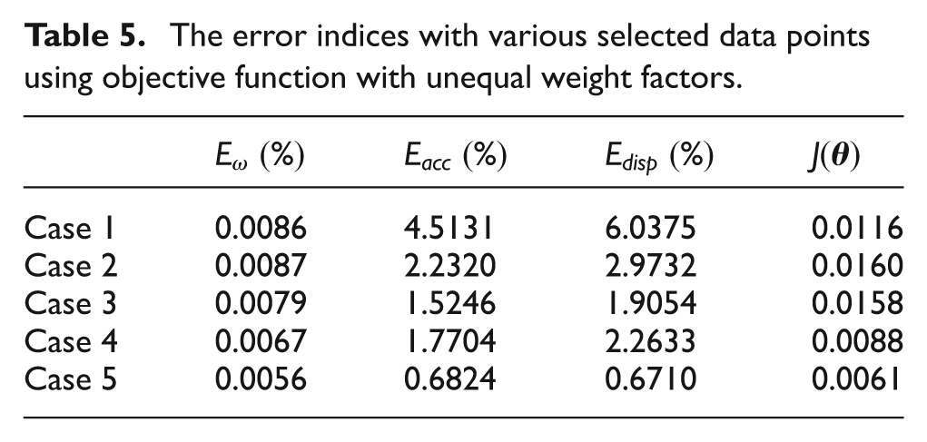
These updated three hysteresis parameters for the above five cases using objective function with equal/unequal weight factors are presented in Tables 2 and 3, respectively, and the corresponding error indices are shown in Tables 4 and 5. From Tables 2 and 3, it can be observed that the nonlinear hysteresis model parameters can be effectively obtained with high accuracy based on the proposed model updating method.

Table 2.

The updated nonlinear hysteretic model parameters with various selected data points using objective function with equal weight factors.

	K₁ (10⁶ kN m)	K₂ (10⁴ kN m)	X (mrad)
Exact	6.867	8.134	3.406
Case 1	6.848 (0.275%)	9.263 (13.884%)	3.752 (10.152%)
Case 2	6.854 (0.195%)	9.255 (13.784%)	3.565 (4.667%)
Case 3	6.858 (0.133%)	8.494 (4.421%)	3.478 (2.115%)
Case 4	6.859 (0.121%)	8.417 (3.476%)	3.482 (2.229%)
Case 5	6.859 (0.114%)	8.329 (2.395%)	3.478 (2.103%)

Table 3.

The updated nonlinear hysteretic model parameters with various selected data points using objective function with unequal weight factors.

	K₁ (10⁶ kN m)	K₂ (10⁴ kN m)	X (mrad)
Exact	6.867	8.134	3.406
Case 1	6.888 (0.304%)	9.009 (10.753%)	3.603 (5.793%)
Case 2	6.846 (0.309%)	8.840 (8.683%)	3.515 (3.194%)
Case 3	6.848 (0.283%)	8.567 (5.322%)	3.475 (2.025%)
Case 4	6.883 (0.235%)	8.258 (1.522%)	3.468 (1.833%)
Case 5	6.853 (0.203%)	8.151 (0.209%)	3.428 (0.661%)

Table 4.

The error indices with various selected data points using objective function with equal weight factors.

	$E_{ω} (%)$	$E_{a c c} (%)$	$E_{d i s p} (%)$	$J (θ)$
Case 1	0.0094	6.5432	8.9441	0.0126
Case 2	0.0060	3.1896	4.4279	0.0167
Case 3	0.0037	1.5183	2.0375	0.0129
Case 4	0.0034	1.5881	2.1318	0.0102
Case 5	0.0032	1.4918	1.9891	0.0079

Table 5.

The error indices with various selected data points using objective function with unequal weight factors.

	$E_{ω} (%)$	$E_{a c c} (%)$	$E_{d i s p} (%)$	$J (θ)$
Case 1	0.0086	4.5131	6.0375	0.0116
Case 2	0.0087	2.2320	2.9732	0.0160
Case 3	0.0079	1.5246	1.9054	0.0158
Case 4	0.0067	1.7704	2.2633	0.0088
Case 5	0.0056	0.6824	0.6710	0.0061

For these cases with equal weight factors, it can be further seen from Figure 7 that all the three indices are smaller than 5% in Cases 3–5 where the numbers of selected data points are not less than 15. With the increase in the number of data points, the defined three error indices show a reducing tendency. However, this reducing trend is not significantly obvious when 20 or more data points are selected. So, for this simulation, 20 data points are enough for calculating instantaneous parameter residuals. Additionally, compared with Case 3, the error indices of Case 5 which shares the same data point number while the distribution is inconsistent are smaller. The updated three parameters of Case 5 are closer to the real values than those of Case 3 (Table 2). This indicates that the local peak values in the uniformly distributed intervals are more representative and reasonable.

Figure 7.

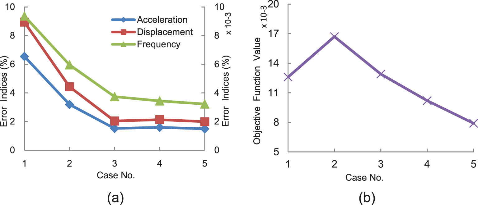
The error indices and objective function values of different cases with equal weight factors: (a) error indices and (b) objective function value.

As shown in Figure 8, the results of cases with unequal weight factors follow almost the same laws discussed above. To discuss the effect of weight factors, the corresponding error indices of Case 5 with unequal weight factors are listed in Table 6, from which we can find that both acceleration and displacement error indices decreased a lot while the frequency still maintained high accuracy. This is mainly caused by the adjustment of weight factors in acceleration and displacement objective functions considering the importance of the maximum displacement and acceleration responses.

Figure 8.

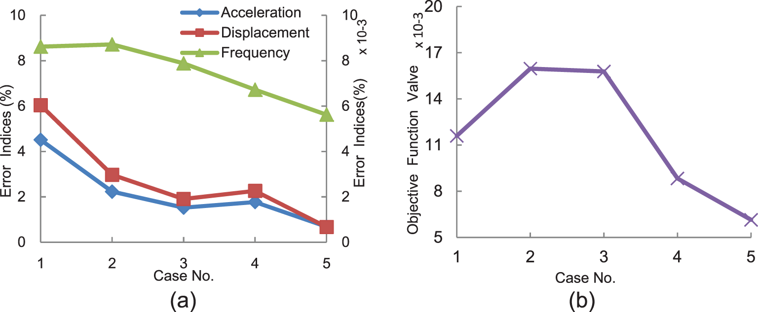
The error indices and objective function values of different cases with unequal weight factors: (a) error indices and (b) objective function value.

Table 6.

The error indices for Case 5 with equal/unequal weight factors.

	$E_{ω} (%)$	$E_{a c c} (%)$	$E_{d i s p} (%)$	$J (θ)$
With equal weight factors	0.0032	1.4918	1.9891	0.0079
With unequal weight factors	0.0056	0.6824	0.6710	0.0061

Therefore, in this article, 20 data points selected at local peaks of the instantaneous characteristics are finally applied for the nonlinear structural model updating using objective functions with unequal weight factors. The comparisons between the updated acceleration responses, displacement responses, and instantaneous frequency and the real values are presented in Figure 9(a) to (c). Also, the nonlinear moment–rotation curve of the updated model is compared with that from baseline model in Figure 10. It can be seen from Figures 9 and 10 that the proposed method can effectively update the nonlinear joint model.

Figure 9.

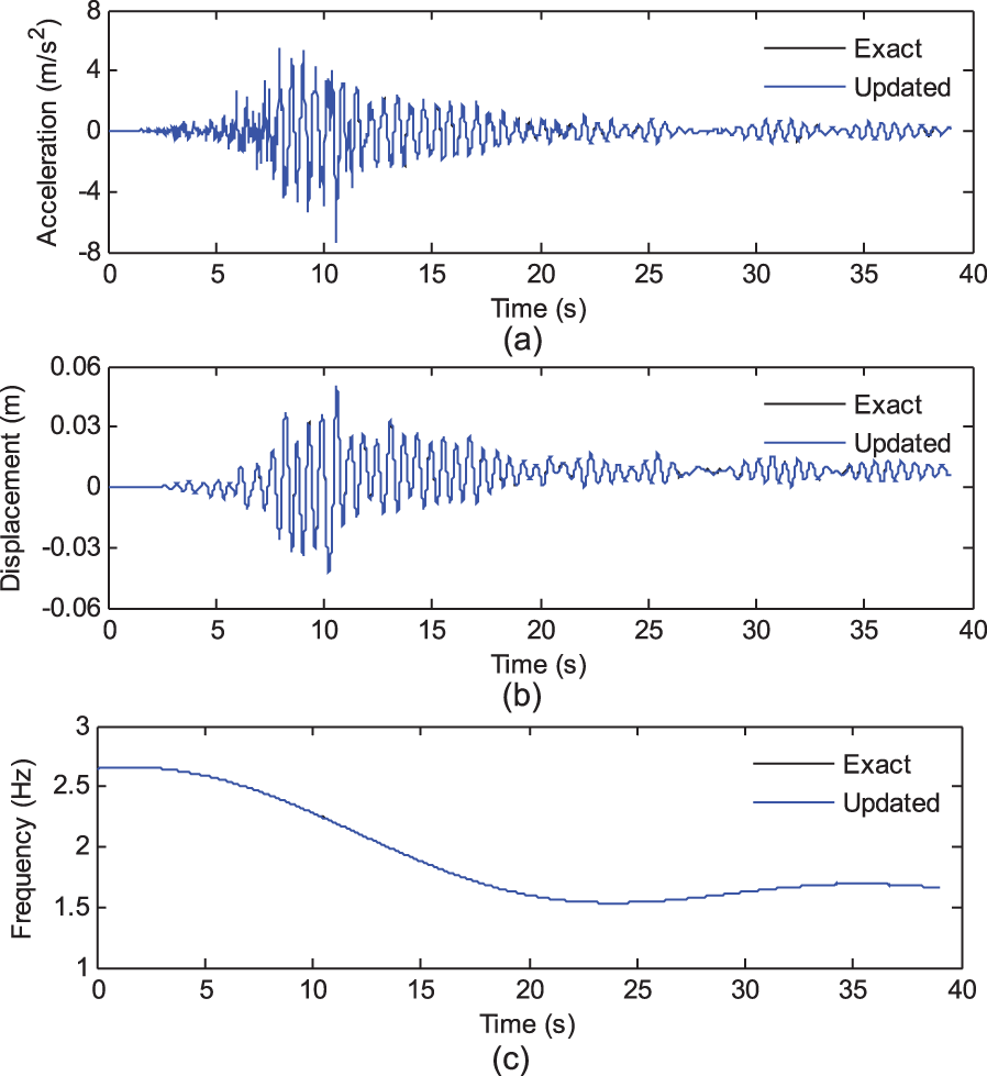
The comparisons between the updated results and the real values without noise: (a) acceleration responses, (b) displacement responses, and (c) frequency.

Figure 10.

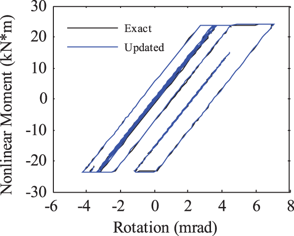
The comparisons of nonlinear moment–rotation hysteretic loops without noise.

Noise effect

To further investigate the robustness of the nonlinear joint model updating framework and its sensitivity to the output measurement noise, 5% and 10% noise-to-signal ratio (NSR) Gaussian white noises are added into the simulated acceleration and displacement as the measured responses, respectively. Again, the method proposed above is carried out to update the nonlinear joint model.

Considering the conclusions drawn from the cases without noise, the three hysteresis parameters K₁, K₂, and X are again updated based on the proposed method with 20 selected local peak values and unequal weight factors. Due to the randomness nature of noise, 100 runs are conducted for different noise levels, respectively. The statistical properties of the updated nonlinear parameters’ relative errors are presented in Table 7, and the corresponding error indices are presented in Table 8. The comparisons between the updated acceleration responses, displacement responses, instantaneous frequency, and the real values during a run are shown in Figures 11 and 13. Also, the corresponding nonlinear moment–rotation curve of the updated model is compared with that from baseline model in Figures 12 and 14.

Table 7.

The relative errors of the updated nonlinear hysteretic model parameters for Case 5 without/with noise effect (%).

		K₁ (10⁶ kN m)	K₂ (10⁴ kN m)	X (mrad)
Without noise		0.203	0.209	0.661
With 5% noise	Min	0.213	1.451	1.097
	Mean	0.397	1.683	1.359
	Max	0.636	1.996	1.725
With 10% noise	Min	1.183	4.131	3.897
	Mean	1.436	4.326	4.156
	Max	1.627	4.632	4.359

Table 8.

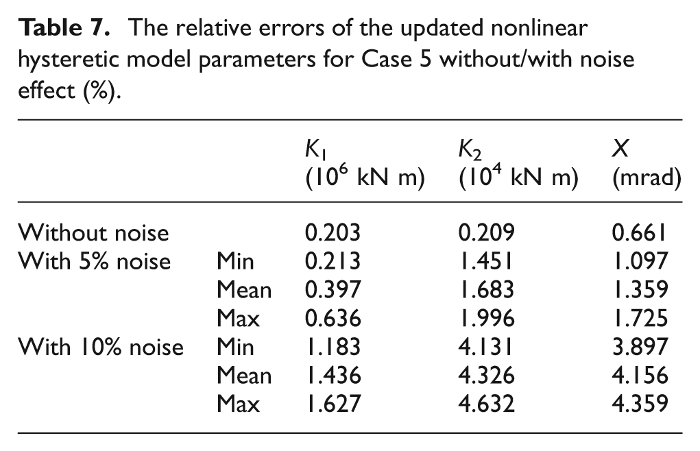
The error indices for Case 5 without/with noise effect.

		$E_{ω} (%)$	$E_{a c c} (%)$	$E_{d i s p} (%)$	$J (θ)$
Without noise		0.0056	0.6824	0.6710	0.0061
With 5% noise	Min	1.0051	2.0123	2.0553	0.0101
	Mean	1.7582	2.3870	2.3524	0.0195
	Max	2.1378	2.7893	2.6391	0.0239
With 10% noise	Min	3.3201	4.6812	4.2695	0.0312
	Mean	4.7743	5.5783	5.3248	0.0391
	Max	6.1929	6.3423	6.1377	0.0586

Figure 11.

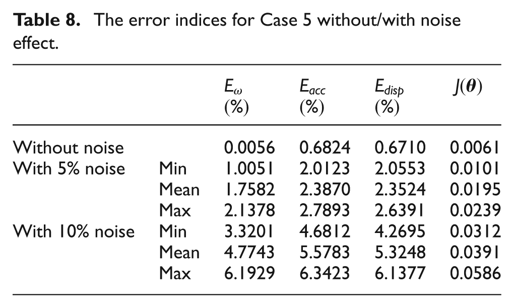
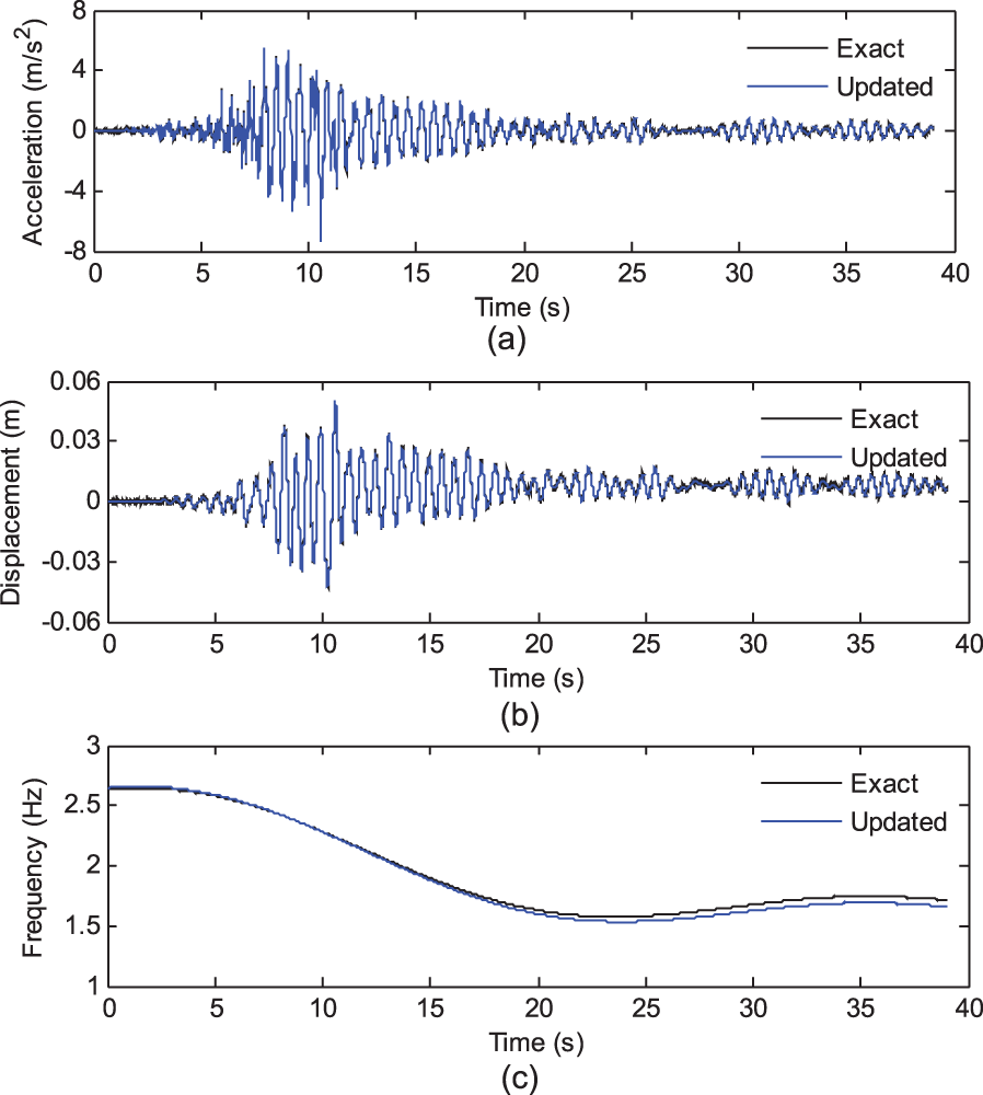
The comparisons between the updated results (during a run) and the real values with 5% noise: (a) acceleration responses, (b) displacement responses, and (c) frequency.

Figure 12.

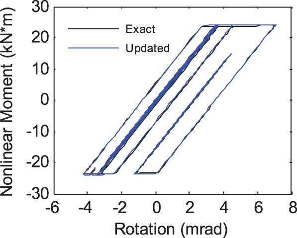
The comparison of nonlinear moment–rotation hysteretic loops with 5% noise (during a run).

It can be observed from Tables 7 and 8 that, for the case with 5% noise, the relative errors of the updated nonlinear hysteretic model parameters (100 runs) are less than 2% and the error indices of frequency, acceleration, and displacement are also less than 3%. When the noise level increases to 10%, the maximum of the error indices is about 6.34% and the mean is less than 5.58%. Figures 11 to 14 show the highly exact fitness between the updated acceleration responses, displacement responses, instantaneous frequency, and the real values. All of these obtained results reveal the high accuracy and robustness of the proposed method.

Figure 13.

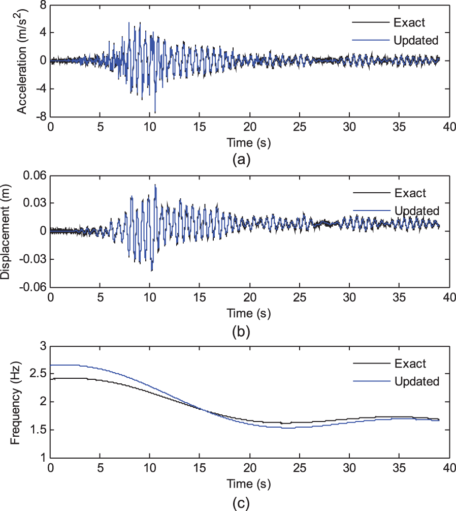
The comparisons between the updated results (during a run) and the real values with 10% noise: (a) acceleration responses, (b) displacement responses, and (c) frequency.

Figure 14.

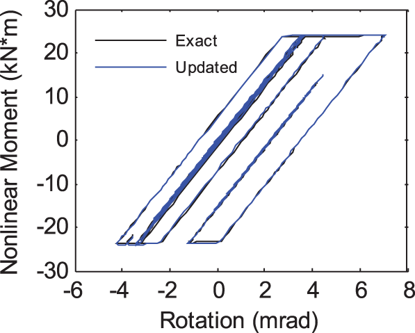
The comparison of nonlinear moment–rotation hysteretic loops with 10% noise (during a run).

Conclusion

This article presents a new nonlinear joint model updating method based on instantaneous frequencies and amplitudes of principal dynamic response components under earthquake excitations. A reasonable objective function based on the residuals of instantaneous frequency and amplitude between experimental structure and FE model is created for nonlinear model updating. The values of the hysteresis parameters are then obtained by minimizing the objective function using simulated annealing algorithm. The effects of the selected data point number, the weight factors in the objective function, and noise effect are also discussed thoroughly. The proposed procedure is validated by the simulation of a three-story frame with bilinear moment–rotation relationship at the beam-column joints. The optimization performs well in the numerical case study. Based on the numerical results, it can be concluded that

The proposed method can effectively update the nonlinear model with high accuracy for numerical simulations. A low level noise has a little effect on the proposed nonlinear joint model updating method.

Limited point values of the instantaneous frequencies and amplitudes can be selected to represent the nonlinear characteristics of the structure and the RS model can be applied to replace the nonlinear FE model.

The created objective function with proposed weight factors and the point values selected method are practical for nonlinear joint model updating.

For real application, the nonlinear structures may perform more complex nonlinear behaviors; thus, the selection of suitable nonlinear models to describe the structural nonlinear behaviors should be further studied.

Footnotes

Declaration of Conflicting Interests

The author(s) declared no potential conflicts of interest with respect to the research, authorship, and/or publication of this article.

Funding

The author(s) disclosed receipt of the following financial support for the research, authorship, and/or publication of this article: Financial support to complete this study was provided, in part, by the National Natural Science Foundation of China under grant nos 51578206 and 51278163, by “The Fundamental Research Funds for the Central Universities”, and by the Natural Science Funds for Distinguished Young Scholar of Anhui Province under grant no. 1708085J06. The results and opinions expressed in this paper are those of the authors only and they do not necessarily represent those of the sponsors.

References

Alamdari

Samali

. (2013) Nonlinear joint model updating in assembled structures. Journal of Engineering Mechanics 140(7): 04014042.

Asgarieh

Moaveni

Stavridis

(2014) Nonlinear finite element model updating of an infilled frame based on identified time-varying modal parameters during an earthquake. Journal of Sound and Vibration 333(23): 6057–6073.

Baruch

Bar Itzhack

(1978) Optimal weighted orthogonalization of measured modes. AIAA Journal 16(4): 346–351.

Berman

Nagy

(1983) Improvement of a large analytical model using test data. AIAA Journal 21(8): 1168–1173.

Box

Wilson

(1951) On the experimental attainment of optimum conditions. Journal of the Royal Statistical Society Series B (Methodological) 13(1): 1–45.

Chen

Wang

(2012) A signal decomposition theorem with Hilbert transform and its application to narrowband time series with closely spaced frequency components. Mechanical Systems and Signal Processing 28: 258–279.

Davoodi

Amiri

Gholampour

. (2012) Determination of nonlinear behavior of a ball joint system by model updating. Journal of Constructional Steel Research 71: 52–62.

Dekkers

Aarts

(1991) Global optimization and simulated annealing. Mathematical Programming 50(1–3): 367–393.

DeSalvo

Swanson

(1989) ANSYS user’s manual. Houston, PA: Swanson Analysis Systems.

10.

Ding

Zhao

. (2015) Simultaneous identification of structural parameter and external excitation with an improved unscented Kalman filter. Advances in Structural Engineering 18(11): 1981–1998.

11.

Ebrahimian

Rodrigo

Joel

(2015) Nonlinear structural finite element model updating and uncertainty quantification. In: Proceedings of the SPIE smart structures and materials nondestructive evaluation and health monitoring, San Diego, CA, 9–13 March.

12.

Fang

(1980) Experimental design by uniform distribution. Acta Mathematice Applicatae Sinica 3: 363–372.

13.

Friswell

Mottershead

(1995) Finite Element Model Updating in Structural Dynamics. Dordrecht: Kluwer Academic Publishers.

14.

Guo

Zhang

(2004) Finite element model updating based on response surface methodology. In: Proceedings of the 22nd IMAC, Dearborn, MI, 26–29 January.

15.

Hasselman

Anderson

Gan

(1998) Principal components analysis for nonlinear model correlation, updating and uncertainty evaluation. In: Proceedings of the 16th international modal analysis conference, Santa Barbara, CA, 2–5 February, pp. 644–651. Bellingham, WA: Society of Photo-Optical Instrumentation Engineers.

16.

Hemez

Doebling

(2001) Review and assessment of model updating for non-linear, transient dynamics. Mechanical Systems and Signal Processing 15(1): 45–74.

17.

Iranzad

Ahmadian

(2012) Identification of nonlinear bolted lap joint models. Computers and Structures 96: 1–8.

18.

Jaishi

Ren

(2005) Structural finite element model updating using ambient vibration test results. Journal of Structural Engineering 131(4): 617–628.

19.

Jaishi

Ren

(2007) Finite element model updating based on eigenvalue and strain energy residuals using multiobjective optimisation technique. Mechanical Systems and Signal Processing 21(5): 2295–2317.

20.

Kirkpatrick

(1984) Optimization by simulated annealing: quantitative studies. Journal of Statistical Physics 34(5–6): 975–986.

21.

Lei

Chen

. (2014) Damage identification of frame structures with joint damage under earthquake excitation. Advances in Structural Engineering 17(8): 1075–1088.

22.

Lenaerts

Kerschen

Golinval

(2001) Proper orthogonal decomposition for model updating of non-linear mechanical systems. Mechanical Systems and Signal Processing 15(1): 31–43.

23.

Link

(1999) Updating of analytical models—review of numerical procedures and application aspects. In: Proceedings of structural dynamics forum (SD2000), Los Alamos, 11–17 April, NM.

24.

Meyer

Link

(2003) Modelling and updating of local non-linearities using frequency response residuals. Mechanical Systems and Signal Processing 17(1): 219–226.

25.

Ren

Chen

(2010) Finite element model updating in structural dynamics by using the response surface method. Engineering Structures 32(8): 2455–2465.

26.

Ren

Fang

Deng

(2010) Response surface–based finite-element-model updating using structural static responses. Journal of Engineering Mechanics 137(4): 248–257.

27.

Schmidt

(1994) Updating non-linear components. Mechanical Systems and Signal Processing 8(6): 679–690.

28.

Shahidi

Pakzad

(2013) Response surface model updating for nonlinear structures. In: Catbas

Pakzad

Racic

. (eds) Topics in Dynamics of Civil Structures, vol. 4. New York: Springer, pp. 283–288.

29.

Silva

(2011) Non-linear model updating of a three-dimensional portal frame based on Wiener series. International Journal of Non-Linear Mechanics 46(1): 312–320.

30.

Silva

Cogan

Foltête

. (2009) Indices for nonlinear model updating in structural dynamics. Journal of the Brazilian Society of Mechanical Sciences and Engineering 31(1): 27–34.

31.

Song

Dyke

Harmon

. (2009) Nonlinear model updating in concrete structures based on ambient response data. In: Proceedings of the 27th international modal analysis conference, Copenhagen, 26–27 April.

32.

Wang

Fang

(1981) A note on uniform distribution and experimental design. Chinese Science Bulletin 26(6): 485–489.

33.

Wang

Chen

(2013) Analytical mode decomposition of a time series with overlapping and rapidly time-varying frequencies with Hilbert transforms. Smart Materials and Structures 22(9): 1–14.

34.

Wang

Ren

Chen

(2013) Time-varying linear and nonlinear structural identification with analytical mode decomposition and Hilbert transform. Journal of Structural Engineering 139(12): 1–5.

35.

Wang

Xin

Ren

(2015) Nonlinear structural model updating based on instantaneous frequencies and amplitudes of the decomposed dynamic responses. Engineering Structures 100: 189–200.

36.

Zhang

Guo

(2007) A case study of model updating and validation of a frame structure with highly non-linear component. In: Proceedings of the 25th international modal analysis conference (CD-ROM), Orlando, 19–22 February.