Effects of friction-based fixed bearings on the seismic vulnerability of a high-speed railway continuous bridge

Abstract

The fixed bearings of high-speed railway continuous bridges were vulnerable during earthquakes, since they transferred most of the seismic force between the superstructure and the piers. A type of friction-based fixed bearing was used and would slide during strong earthquakes. The influence of this sliding friction action on the seismic vulnerability curves of different components in the track-bridge system was analyzed in this article. Results show that the sliding friction action of the fixed bearings can protect other components from severe damage under earthquakes. This phenomenon is more significant when the friction coefficient on the friction-based fixed bearings is reduced. However, it increases the seismic relative displacement of the fixed bearings themselves. Finally, a sufficiently large displacement capacity and an appropriate friction coefficient between 0.2 and 0.3 are almost the best combination for the friction-based fixed bearings, which can effectively protect all components of the track-bridge system, including the track structure, piers, piles, and friction-based fixed bearings themselves.

Keywords

bearings continuous bridge friction high-speed railway relative displacement seismic vulnerability

Introduction

A typical high-speed railway continuous bridge contains many sliding bearings and a few fixed bearings in the longitudinal direction. In an earthquake, most of the inertia forces are transferred from the superstructure to the piers through the fixed bearings. Those fixed bearings are prone to seismic damage among all of the bridge components (Pan et al., 2010) and are paid more attentions by different researchers. For example, based on experimental results from Mander et al. (1996) and Randall et al. (1999) and the displacement-based damage index, Choi et al. (2004) defined five damage states from an intact state to a complete damage state for the fixed bearings. And other similar damage states of the fixed bearings were also defined based on the displacement index (Nielson and DesRoches, 2007; Padgett and DesRoches, 2008), the shear strain index (Taskari and Sextos, 2015), and the friction coefficient index (Kim et al., 2006).

Based on the full bridge finite element (FE) model analysis and the bearing experiment, Steelman et al. (2014) found that the ultimate damage state of the fixed steel bearings considerably influenced the seismic performance of the bridge structure. In terms of the high-speed railway continuous bridge, there was a significant track–bridge interaction (Dai and Liu, 2013; He et al., 2017; Zhang et al., 2015), and the damage states and the residual capacity of the fixed bearings would significantly influence the seismic vulnerability of the track system and the bridge system. However, the latter was lack of deep investigation. In recent years, more attentions have been paid for the train safety under earthquakes (Chen et al., 2014; Du et al., 2012; Ju, 2013; Zeng et al., 2015) instead of the seismic track–bridge interaction. The effects of the bearing damage on the seismic behavior of the ballastless track–bridge system need further research.

Fortunately, seismic vulnerability analysis provided an effective method to evaluate those effects of the bearing damage on the seismic performance of the track–bridge system, although it had not yet been done now. Compared with an empirical method (Shinozuka et al., 2000a) using real seismic damage data and aiming at specific situations, a theoretical method (Karim and Yamazaki, 2001; Shinozuka et al., 2000b) could be widely used to get seismic vulnerability curves of any bridge types at any sites (Padgett and DesRoches, 2008) since the structural seismic responses were theoretically calculated (Karim and Yamazaki, 2003). For example, Choi et al. (2004) established the vulnerability curves of key members and the full bridge system for six bridge categories in the southeast and central parts of United States and provided different reinforcements to improve the seismic vulnerability. Nielson and DesRoches (2007) proposed seismic vulnerability relations among piers, abutments, and bearings. Ramadan et al. (2015) and Taskari and Sextos (2015) analyzed the influence of the spatial variability of ground motion on the seismic vulnerability of bridges on different types of foundation soil. All of the researches above show that the fixed bearings are prone to seismic damage, however, only aiming at the highway bridges instead of the high-speed railway bridges with considerable track–bridge interaction.

The previous experiment showed that the fracture of the common fixed bearings was uncertain (Steelman et al., 2014), and a lot of assumptions had to be adopted for the seismically damaged fixed bearings, which would possibly lead to untrue or irregular responses of the bridge system (Wei et al., 2015). Wei et al. (2017) investigated a type of friction-based fixed bearing, which could reliably connect the girder and the pier by a large friction force under common loads, and would slide when the friction force was overcome by the inertia force under strong earthquakes. It is easy and reliable to simulate this friction-based fixed bearing with less uncertain factors. This article analyzes the effects of this friction-based fixed bearing, with different friction coefficients and displacement capacities, on the seismic vulnerability curves of different components in a typical high-speed railway continuous bridge with ballastless track.

Track–bridge structure

Introduction of a railway bridge

A typical pre-stressed concrete continuous bridge with three spans of (48 + 80 + 48) m on a high-speed railway is shown in Figure 1. The girder cross-section is shown in Figure 2, and its concrete adopts C50. The largest and smallest heights of the girder are 6.65 and 3.85 m, respectively, and its bottom line is quadratic parabola as shown in Figure 1. The bearing distribution is shown in Figure 3, and all of the bearings are the friction-based ones, including the sliding bearings and the fixed bearings. The sliding bearings have a small friction coefficient and can slide under common loads. The fixed bearings can reliably connect the girder and the pier by a large friction force under common loads, however, can also slide under strong earthquakes. As for the piers made of C30 concrete, 7.6 × 3.4 m rectangular cross-section is chosen for No. 1 and No. 4 piers, while 8.6 × 4.2 m rectangular cross-section is chosen for No. 2 and No. 3 piers. In terms of the piles made of C30 concrete, the pile foundation at the bottom of No. 1 and No. 4 piers is respectively composed of 16 circular piles with diameter of 1.25 m, while the pile foundation of No. 2 and No. 3 piers is respectively composed of 20 circular piles with diameter of 1.5 m.

Figure 1.

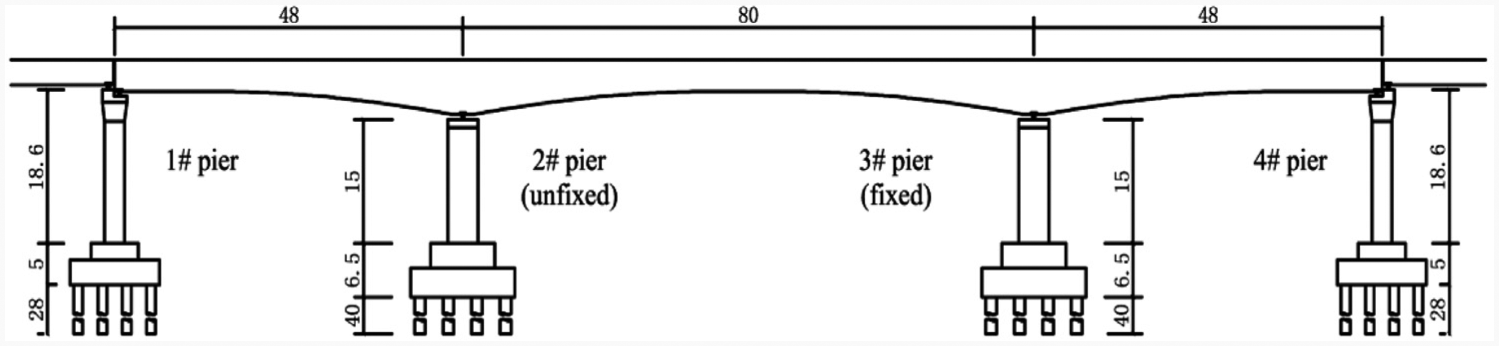
The layout of the full bridge (m).

Figure 2.

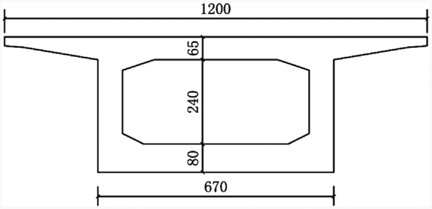
Cross-section of girder (mm).

Figure 3.

Bearing restraint and distribution.

Ballastless slab track adopts the China Railway Track Slab II (CRTSII), consisting of sliding layer, shear teeth, block, base plate, cement asphalt (CA) layer, shear bars, track plate, fasteners, rails, and other components. The track plate and the base plate are continuous across girder gaps. Most parts of the base plate can freely slide on the sliding layer set on the girder, while some parts are fixed to the girder part on the top of the fixed bearings by the shear teeth as shown in Figure 4. The track plate and the base plate are connected with each other by the CA layer at the common positions and by the shear bars at the ends of girder as shown in Figure 4. Many lateral blocks are directly set on the girder and provide the transverse boundary restriction of track structure and ensure the vertical buckling stability of track structure.

Figure 4.

Schematic sketch of the track structure.

Finite element model

A ballastless track-bridge model is built by Open System for Earthquake Engineering and Simulation (OpenSEES) as shown in Figure 5. The girder, the base plate, the track plate, and the rail are simulated by the elastic beam element. The friction-based bearing, the sliding layer, the CA layer, and the fastener are simulated by different zero-length non-linear connecting elements. For example, the friction-based bearings and the sliding layer are simulated by the single friction pendulum bearing (FPB) elements with a very large curvature radius (Wei et al., 2016). The CA layer, the fastener, the shear teeth, the block, and the shear bars are simulated by the Elastic-Perfectly Plastic uniaxial Material elements (Yu, 2015; Zhang et al., 2015). The piers and the piles are simulated by non-linear fiber element. Their stress–strain curves of the confined concrete, the un-confined concrete, and the steel bars are shown in Figure 6. The pile–soil interactions are simulated by the springs. Three-span (32 × 3 m) simply supported girder bridges are built on each side of the continuous bridge to simulate the boundary conditions.

Figure 5.

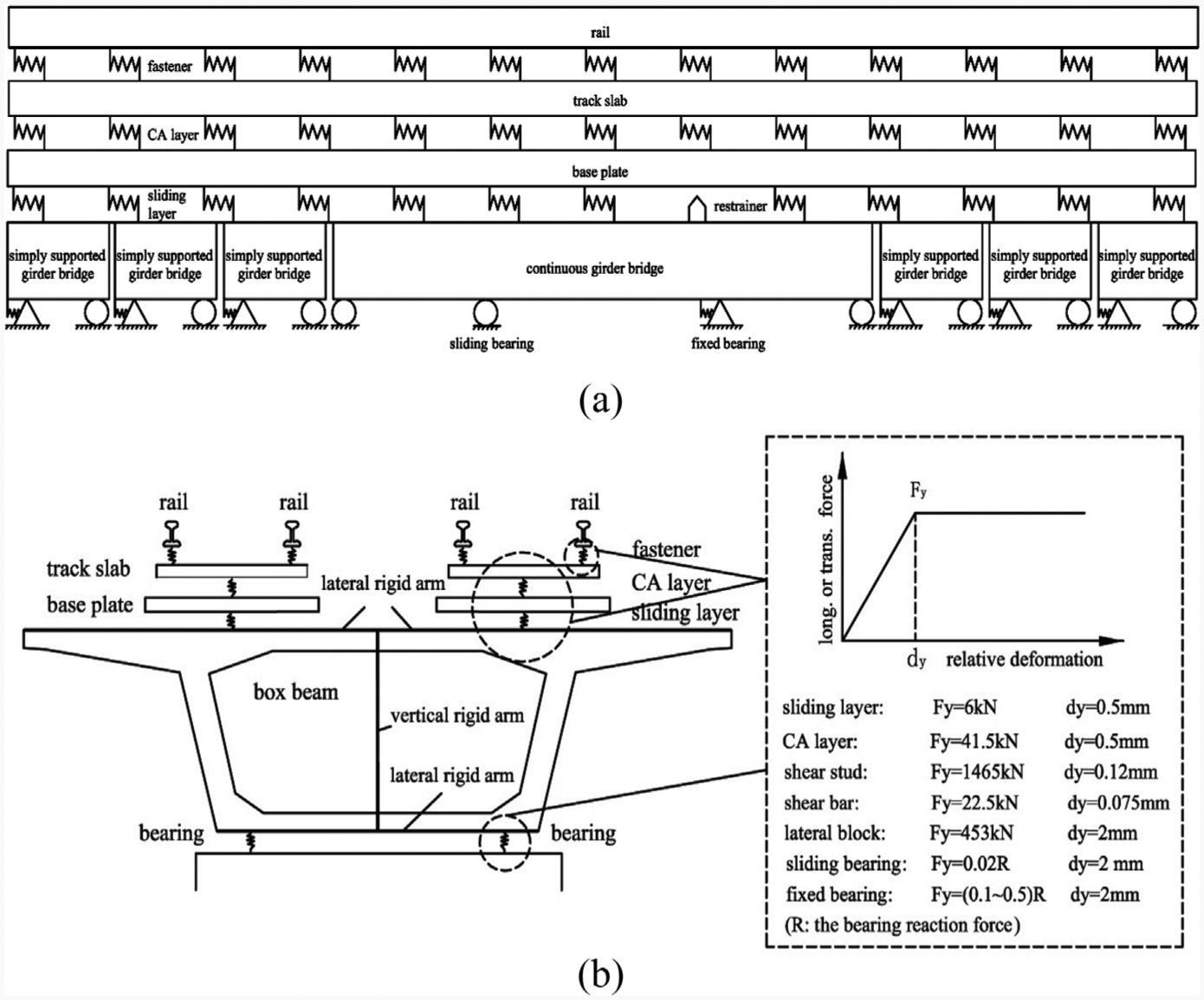
Finite element model of the track structure (Yu, 2015): (a) longitudinal dynamic model and (b) transverse dynamic model.

Figure 6.

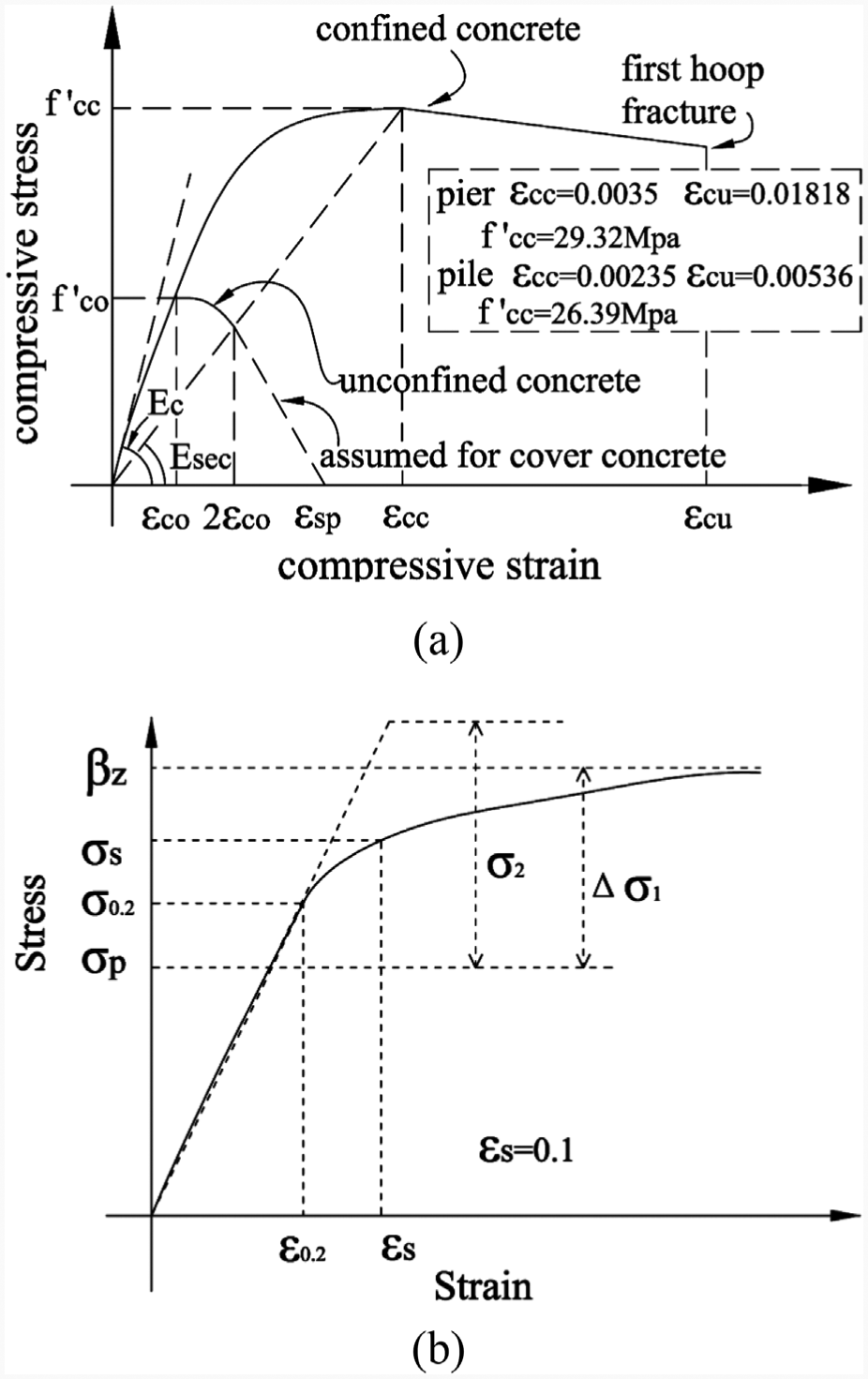
Stress–strain curves of the material of piers and piles: (a) concrete material model and (b) steel material model.

Based on the description above, the track structure is considered in detail and almost all of the potentially damaged components are simulated by non-linear elements in the track–bridge FE model, which are obviously different from the previous investigations. This article focuses on the effects of the non-linear behavior of friction-based fixed bearings on the seismic vulnerability curves of different components in the track–bridge system, by temporarily ignoring the train with different speeds.

Calculation process

Vulnerability analysis method

Seismic vulnerability is defined as the conditional probability that the seismic demand (D) of the structure exceeds the capacity limit (C) of a damage state when the intensity measure (IM) is a specified value. It can be expressed as follows

P_{failure} = P [D \geq C | IM]

(1)

D is usually assumed to obey the lognormal distribution (Cornell et al., 2002) and is the function of IM as follows

S_{d} = aI M^{b}

(2)

where a and b are obtained through regression analysis on a large number of seismic response data.

In equation (1), C is expressed by the structural different damage limit states (LS), which is also assumed to obey the lognormal distribution. Therefore, equation (1) can be further expressed as follows

P [D \geq C | IM] = Φ (\frac{\ln (S_{d} / S_{c})}{\sqrt{β_{d}^{2} + β_{c}^{2}}})

(3)

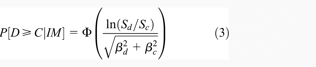
In equation (3), the median values and the logarithmic standard values of D and C are expressed by S_d and S_c, and β_d and β_c, respectively. Φ is the standard normal distribution function.

The specific steps of the seismic vulnerability analysis in this article are described as follows:

Step 1. Select a suite of ground motion records according to the soil profile at the bridge site and scale them to different seismic intensity (IM) levels.

Step 2. Model bridges and calculate seismic responses, i.e. engineering demand parameters (EDPs), using incremental dynamic analysis (IDA) method (Vamvatsikos and Cornell, 2002).

Step 3. Generate the relationship between EDP and IM for the critical components of the bridge based on equation (2).

Step 4. Choose proper seismic damage criterion and assign damage LS.

Step 5. Develop fragility curves for bridge components by comparing EDP and LS based on equation (3).

Earthquake input

The seismic hazard assessment report shows that the soil with shear wave velocity above 500 m/s is very thick for the bridge site, and the characteristic period of earthquake spectrum is 0.25 s. By assuming the damping ratio to be 0.05 for the concrete bridge, the dynamic amplification factor of earthquake spectrum is about 2.25. However, this bridge site is lack of historically recorded ground motions. As to match the assessed earthquake spectrum of the bridge site, 20 pairs of ground motion recordings are selected and scaled from the Pacific Earthquake Engineering Research Center database and are listed in Figure 7. Those well-matched ground motion recordings will be further scaled to obtain the waves with different intensities for the IDA analysis of the bridge models.

Figure 7.

Ground motion input.

With the suggestion by researchers (Vamvatsikos and Cornell, 2005), both the peak ground acceleration (PGA) and the spectral acceleration (Sa) are most commonly used seismic IMs of the IDA analysis to get the EDPs. The study findings of Vamvatsikos and Cornell (2005) further indicated that Sa performed better than PGA in order to reduce the dispersion of the IDA results. Therefore, Sa was temporarily assumed to be the optimum choice of IM for the track–bridge structure model in this study.

Briefly, the spectral acceleration (Sa) is defined as the PGA of the starting point of the average spectrum in Figure 7. This PGA is respectively adjusted to be 0.05, 0.1, 0.2, 0.4, and 0.8 g to represent five different IM levels, and other points of the average spectrum in Figure 7 are scaled with the same scale factors. Accordingly, the acceleration values of all accelerograms in Figure 7 are also adjusted by the same scale factors to get the direct ground motions of IDA analysis.

This article only focuses on the longitudinal seismic performance of the track–bridge structure, and 100 cases are generated for the further calculation by combining 20 pairs of ground motion recordings and five different IM levels. By further considering five different friction coefficients and five different displacement capacities of the friction-based fixed bearings which are described in section “Interaction between capacity and demand of the fixed bearings,” there are 2500 calculation cases in total.

For the 2500 calculation cases above, a great many of seismic responses are obtained. The following sections discuss those results, but only classical and common results are discussed in detailed manner due to space limitations while other results are considered but not listed.

Component LS

The studies (Hwang et al., 2000; Park and Ang, 1985) show that the damage states, from the intact state to the completely destroyed state, of the components can be objectively described by one of the most appropriate parameters, such as the material strain, the section curvature, and the component displacement.

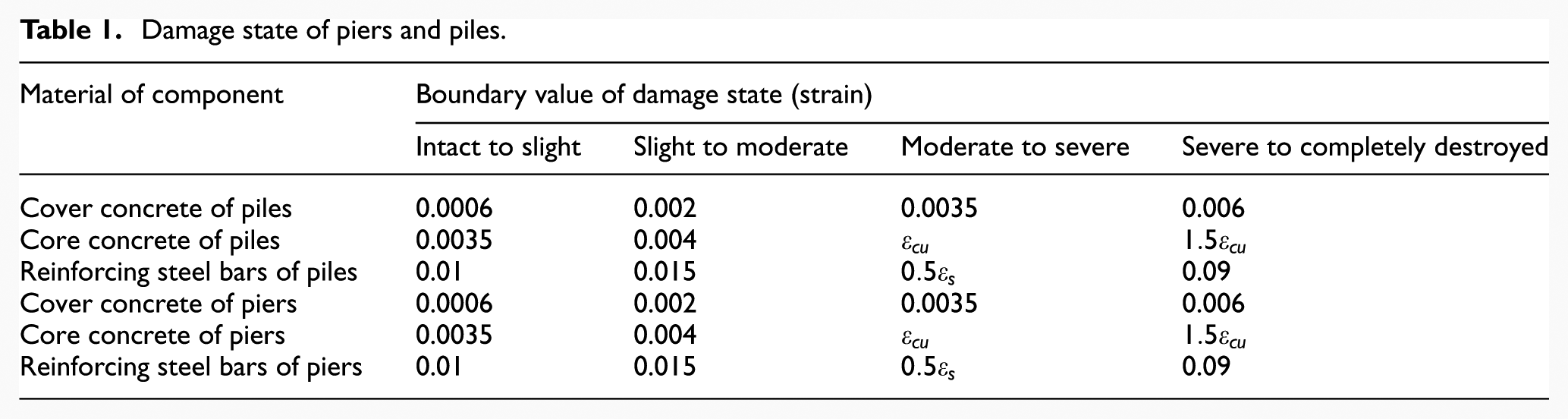
The piers and the piles are simulated by non-linear fiber element. The stress–strain curves of the confined concrete, the un-confined concrete, and the steel bars are shown in Figure 6. The material strain can be used to define the capacity LS of those components (Kowalsky, 2002), which are shown in Table 1. In Table 1, $ε_{cu}$ and $ε_{s}$ are the ultimate strains of core concrete and steel bars as shown in Figure 6(b) and (c), respectively.

Table 1.

Damage state of piers and piles.

Material of component	Boundary value of damage state (strain)
Material of component	Intact to slight	Slight to moderate	Moderate to severe	Severe to completely destroyed
Cover concrete of piles	0.0006	0.002	0.0035	0.006
Core concrete of piles	0.0035	0.004	$ε_{cu}$	$1.5 ε_{cu}$
Reinforcing steel bars of piles	0.01	0.015	$0.5 ε_{s}$	0.09
Cover concrete of piers	0.0006	0.002	0.0035	0.006
Core concrete of piers	0.0035	0.004	$ε_{cu}$	$1.5 ε_{cu}$
Reinforcing steel bars of piers	0.01	0.015	$0.5 ε_{s}$	0.09

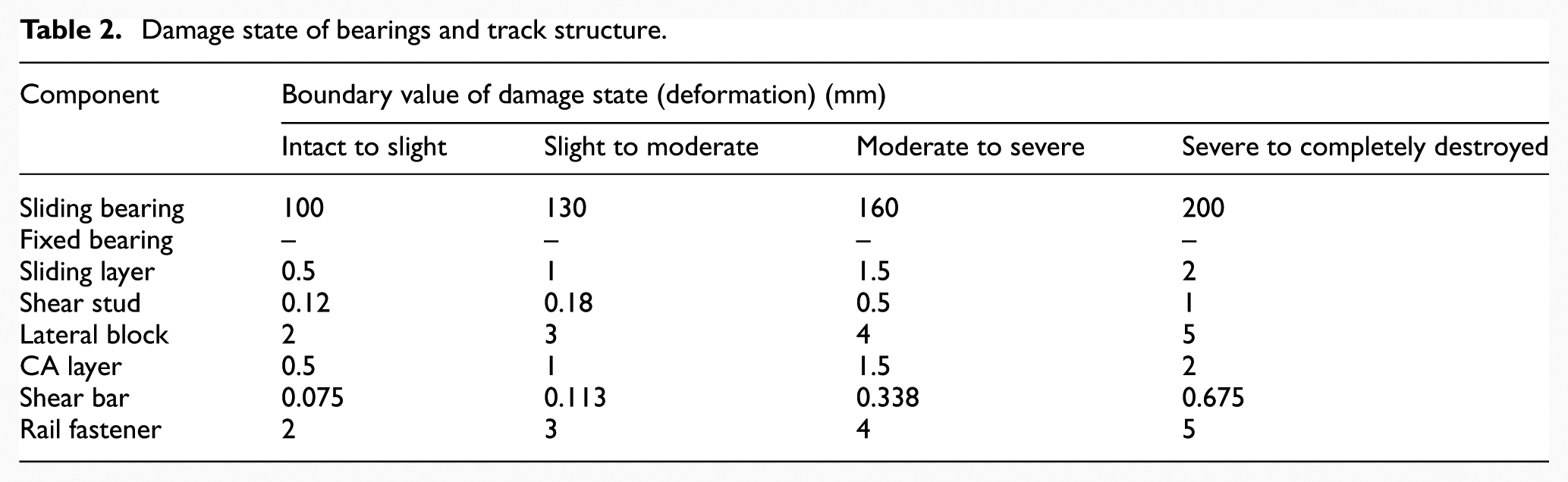
The bearing, the sliding layer, the CA layer, and the fastener are simulated by the zero-length non-linear connecting element, as shown in Figure 5. The relative displacement can be used to define the capacity LS of those components (Yu, 2015; Zhang et al., 2015), which are shown in Table 2 except for the fixed bearings. It is necessary to explain that the parameter values in Table 2 are very conservative due to the lack of enough support of test data.

Table 2.

Damage state of bearings and track structure.

Component	Boundary value of damage state (deformation) (mm)
Component	Intact to slight	Slight to moderate	Moderate to severe	Severe to completely destroyed
Sliding bearing	100	130	160	200
Fixed bearing	–	–	–	–
Sliding layer	0.5	1	1.5	2
Shear stud	0.12	0.18	0.5	1
Lateral block	2	3	4	5
CA layer	0.5	1	1.5	2
Shear bar	0.075	0.113	0.338	0.675
Rail fastener	2	3	4	5

Interaction between capacity and demand of the fixed bearings

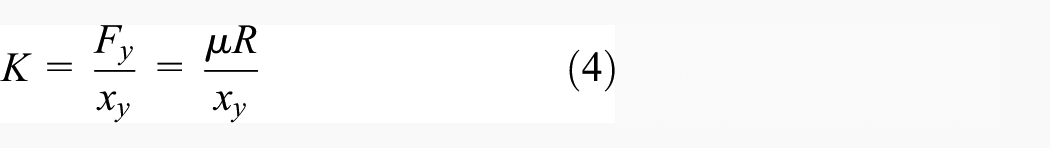
The friction-based fixed bearings are composed of the un-sliding state and the sliding state and are simulated by the single FPB elements elements with a very large curvature radius (Wei et al., 2016). Under common loads, the static friction force on the fixed bearings causes the relative deformation between the girder and the pier. When the relative deformation reaches the peak value x_y of 2 mm, the static friction force is assumed to reach the peak value F_y, which is further assumed to be equal to the sliding friction force under strong earthquakes. And thus the initial stiffness K of the fixed bearings can be expressed as follows

K = \frac{F_{y}}{x_{y}} = \frac{μ R}{x_{y}}

(4)

where $μ$ is the sliding friction coefficient and R is the bearing reaction force.

During strong earthquakes, the friction-based fixed bearings slide like sliding bearings. Simultaneously, they get a much larger friction coefficient from 0.1 to 0.5, which depends on the roughness of friction interface. Their initial stiffness K, calculated by equation (4), is shown in Table 3. The relationship between the median value S_d of the bearing relative displacement demand and the seismic intensity index IM is calculated by equation (2), and its logarithm form is shown as follows

Table 3.

Initial stiffness of the fixed bearings.

	CASE1	CASE2	CASE3	CASE4	CASE5
Friction coefficient	0.1	0.2	0.3	0.4	0.5
Initial stiffness of the fixed bearing at 3# pier (kN/m)	1,175,000	2,350,000	3,525,000	4,700,000	5,875,000
Initial stiffness of the fixed bearing of simply supported bridges (kN/m)	145,000	290,000	435,000	580,000	725,000

\ln (S_{d}) = \ln (a) + b \ln (IM)

(5)

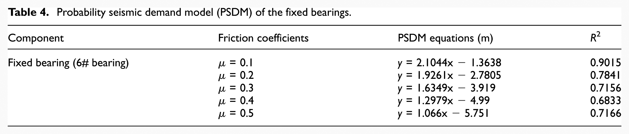
The results of equation (5) and the coefficient R², indicating the accuracy of fit, are shown in Table 4. When those results are compared with LS, seismic vulnerability curves are obtained for the fixed bearings. This fragility analysis process is also applicable for other components of the track–bridge system.

Table 4.

Probability seismic demand model (PSDM) of the fixed bearings.

Component	Friction coefficients	PSDM equations (m)	R ²
Fixed bearing (6# bearing)	μ = 0.1	y = 2.1044x − 1.3638	0.9015
	μ = 0.2	y = 1.9261x − 2.7805	0.7841
	μ = 0.3	y = 1.6349x − 3.919	0.7156
	μ = 0.4	y = 1.2979x − 4.99	0.6833
	μ = 0.5	y = 1.066x − 5.751	0.7166

In Table 5, CASE(a) shows the common seismic damage states, defined by the relative displacement, of the friction-based fixed bearings. The bearing states are divided into the un-sliding state and the sliding state. The un-sliding state implies an intact state for the bearings, while the sliding state means different damage states. However, a small relative displacement can still be acceptable, while a larger relative displacement implies a much more possible change of the bearing mechanics, such as the instability and the overturning of the bearings. Those damage states in CASE(a) are used to calculate the results as shown in section “Influence of friction coefficients of fixed bearings on fragilities.” The relative displacement capacities in CASE(b), CASE(c), CASE(d), and CASE(e) increase in different ways when comparing with that in CASE(a). Those varieties only change the fragility curves of the fixed bearings themselves in theory, which is obviously different from the effects of the variable friction coefficient on the fixed bearings. And the corresponding results are shown in section “Influence of displacement capacities of fixed bearings on fragilities.”

Table 5.

Displacement capacity of the fixed bearings (m).

Boundary cases	CASE(a)	CASE(b)	CASE(c)	CASE(d)	CASE(e)
Intact to slight	0.002	0.002	0.002	0.002	0.002
Slight to moderate	0.004	0.006	0.006	0.006	0.008
Moderate to severe	0.006	0.008	0.01	0.01	0.014
Severe to completely destroyed	0.008	0.01	0.012	0.014	0.02

Influence of friction coefficients of fixed bearings on fragilities

Fixed bearing

When the friction-based fixed bearings slide during earthquakes, an increase of the friction coefficient on them, as shown in Table 4, significantly reduces the damage level of themselves as shown in Figure 8. For example, when the friction coefficient increases from 0.1 to 0.5 in the case of PGA = 1.0g, the probabilities exceeding the slightly damaged state as shown in Figure 8(b) are 1, 1, 1, 0.86, 0.32, respectively, and the probabilities exceeding the severely damaged state as shown in Figure 8(d) are 1, 1, 0.96, 0.37, 0.03, respectively. The reason is that an increase of the friction coefficient or the friction force on the fixed bearings can dissipate the earthquake energy more efficiently and further reduce the relative displacement and the damage level of the fixed bearings between the girder and the pier.

Figure 8.

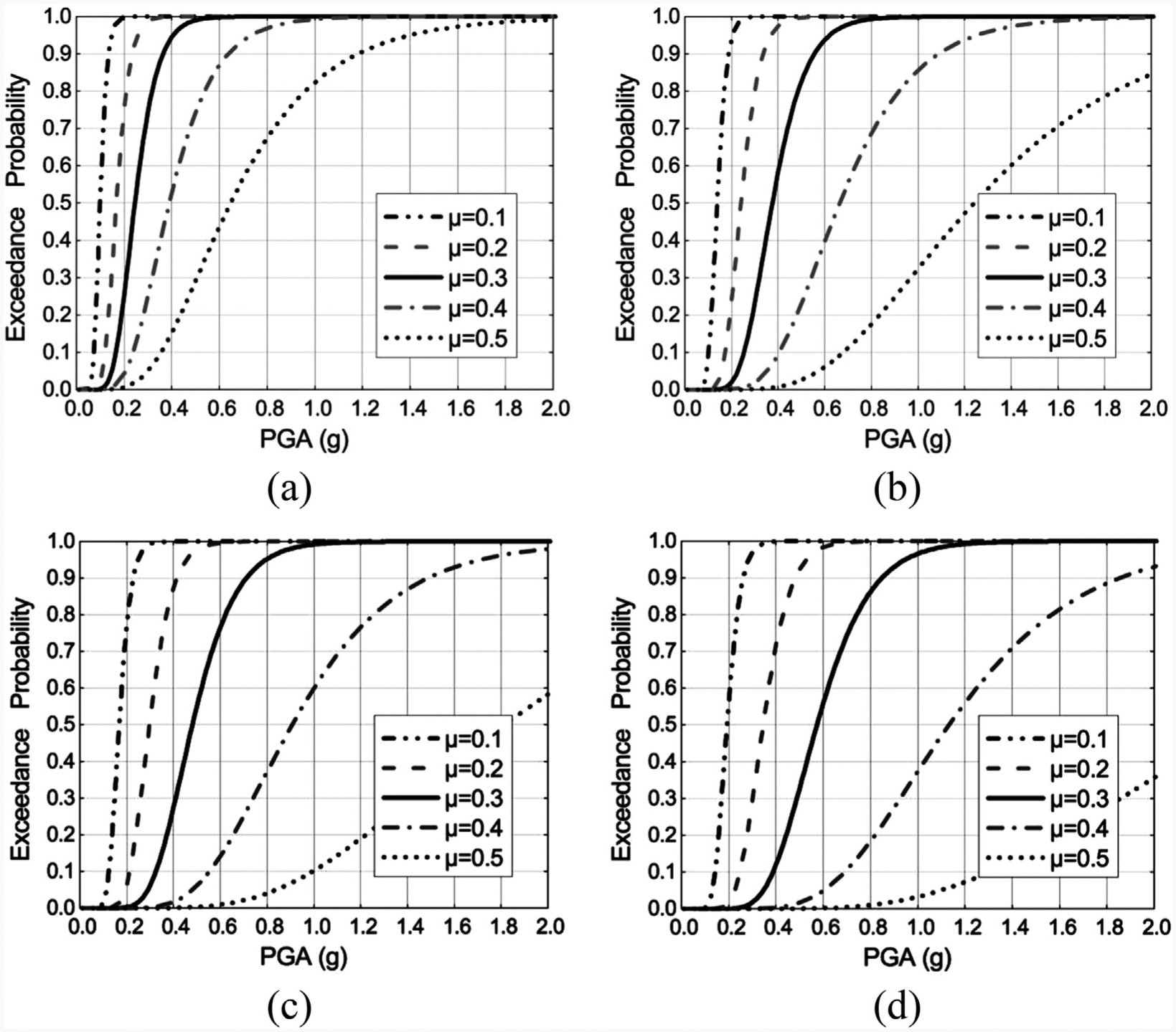
Influence of friction coefficients of fixed bearings on fragility curves for fixed bearings: (a) exceeding intact state, (b) exceeding slight damage state, (c) exceeding moderate damage state, and (d) exceeding severe damage state.

When the relative displacement and the damage level of the fixed bearings are larger, the energy dissipation function of the bearing friction action is more significant. In this condition, an increase of the friction coefficient on the fixed bearings will reduce the damage level of themselves more considerably. For example, when the friction coefficient increases from 0.4 to 0.5 in the case of PGA = 1.0g, the probabilities exceeding four different damage states, from the intact state to the severely damaged state as shown in Figure 8(a) to (d), are reduced by 17%, 63%, 83%, and 92%, in which the reduced ratios increase rapidly.

Sliding bearing

Because the sliding bearings are connected with the fixed bearings by an elastic girder, an increase of the friction coefficient on the fixed bearings will reduce the relative displacement and the damage level of the sliding bearings as well as the fixed bearings. It can be validated by the seismic fragility curves of the sliding bearings as shown in Figure 9. For example, when the friction coefficient on the fixed bearings increases from 0.1 to 0.5 in the case of PGA = 1.0g, the probabilities exceeding the slightly damaged state of the sliding bearings as shown in Figure 9(b) are 0.93, 0.82, 0.73, 0.70, and 0.69, respectively, and the probabilities exceeding the severely damaged state as shown in Figure 9(d) are 0.72, 0.52, 0.4, 0.37, and 0.36, respectively. It is noted that the exceedance probabilities of the sliding bearings decrease more slowly with the increase of friction coefficients of the fixed bearings, and this phenomenon is different from the fixed bearings themselves as shown in Figure 8.

Figure 9.

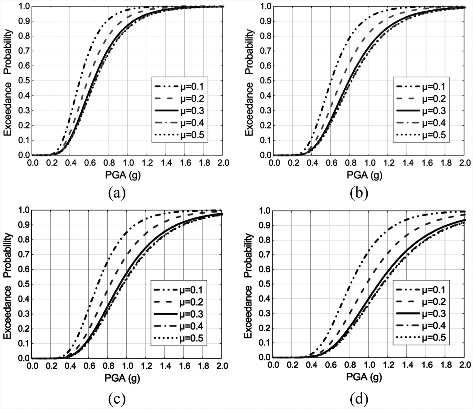
Influence of friction coefficients of fixed bearings on fragility curves for sliding bearings: (a) exceeding intact state, (b) exceeding slight damage state, (c) exceeding moderate damage state, and (d) exceeding severe damage state.

By comparing Figures 8 with 9, it is obvious that the fixed bearings are more vulnerable to be seismically destroyed than the sliding bearings for most cases. However, this rule becomes opposite when the friction coefficient on the fixed bearings increases to a certain value.

Track structure

Figure 10 shows the average value of the maximum longitudinal deformations of the track structure, including the sliding layer, the CA layer, and the fastener, for the case with the friction coefficient of 0.2 on the fixed bearing under different earthquakes.

Figure 10.

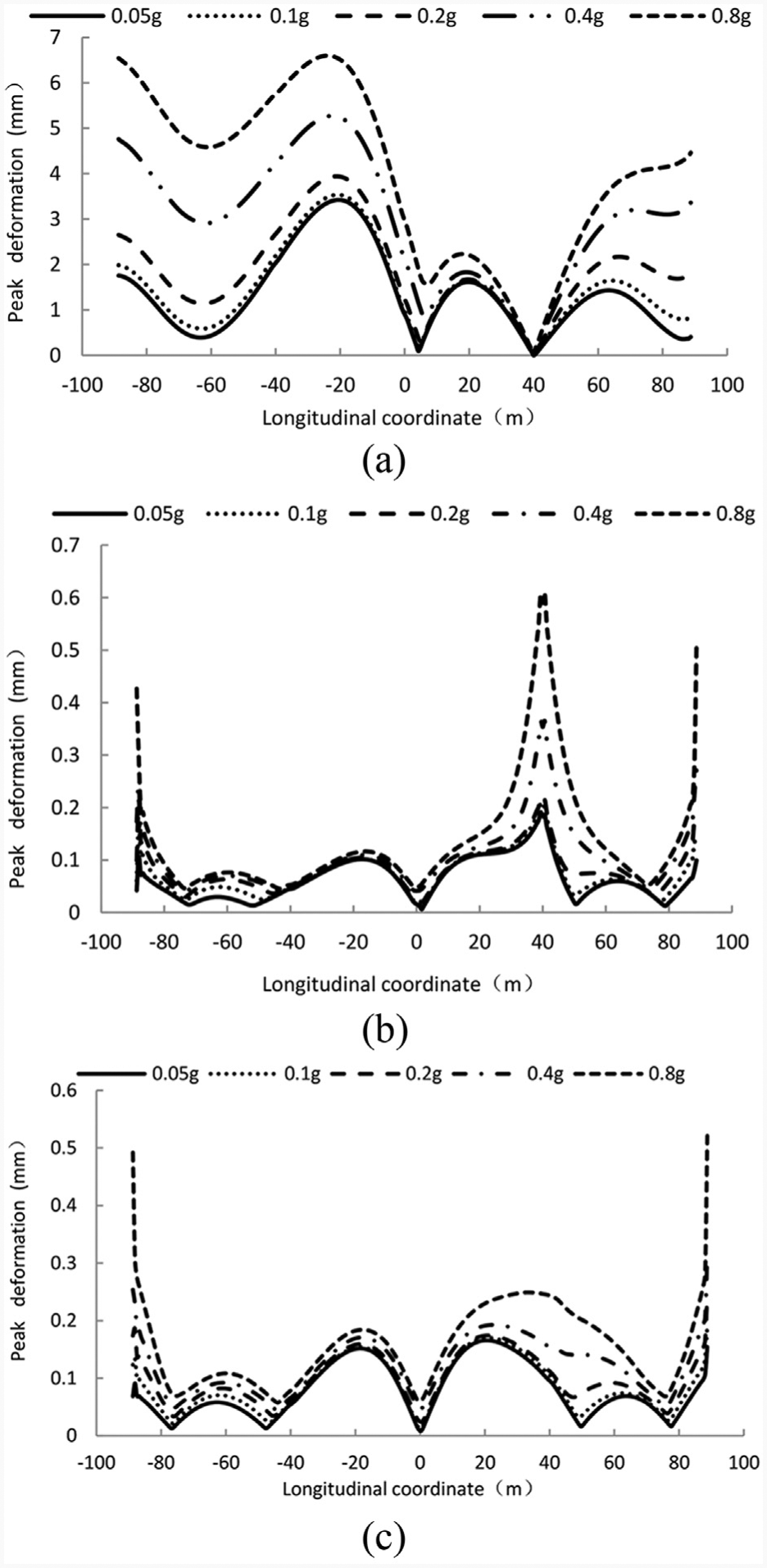
Peak deformations of the track structure in the longitudinal direction ( $μ = 0.2$ ): (a) sliding layer, (b) CA layer, and (c) fastener.

It is shown in Figure 10(a) that almost all maximum longitudinal deformations of sliding layers are beyond the slight damage of 0.5 mm. It is indicated that the sliding layers are very vulnerable to seismic damages. Furthermore, when PGA ≥ 0.4, most of sliding layers are in danger of collapse, and more protection measures should be taken to use. Because of the fixed constraint of shear teeth on the top of 3# pier, the base plate there moves along with the girder. Therefore, there is no relative displacement between the base plate and the girder over there, and the maximum longitudinal deformation of sliding layer there remains zero under the seismic loading. However, it will transmit more seismic energy to the CA layer and cause the significant peak deformation of the CA layer there as shown in Figure 10(b). Due to the uncoordinated deformation near the end of girder, the maximum longitudinal deformations of sliding layers, the CA layers and the fasteners there reach the local peak values, and significantly increase with PGA.

From Figure 10, CA layers and fasteners in the track structure are protected by the sliding action of the sliding layer during an earthquake and only have an ignored damage level. And thus the influence of the uncertain friction action of the fixed bearings on the seismic fragility curves of those components is feeble.

However, the sliding action of the sliding layer implies a damage existing in the sliding layer, although it can dissipate earthquake energy. When the friction coefficient on the fixed bearings increases, the earthquake energy transferred from the fixed pier to the girder will be larger and will enlarge the damage level of the sliding layer. For example, the fragility curves of the sliding layer near 1# pier are shown in Figure 11. When the friction coefficient on the fixed bearings increases from 0.1 to 0.5 in the case of PGA = 0.5g, the probabilities exceeding the slightly damaged state as shown in Figure 11(b) are 0.96, 1, 1, 1, 1, respectively, and the probabilities exceeding the severely damaged state as shown in Figure 11(d) are 0.66, 0.91, 0.95, 0.96, 0.97, respectively. Those exceedance probabilities increase more significantly for the severe damage state, especially when the friction coefficient on the fixed bearings increases from 0.1 to 0.2.

Figure 11.

Influence of friction coefficients of fixed bearings on fragility curves for the sliding layer: (a) exceeding intact state, (b) exceeding slight damage state, (c) exceeding moderate damage state, and (d) exceeding severe damage state.

Pier

The piers are simulated by non-linear fiber element, which is composed of the confined concrete, the un-confined concrete, and the steel bars. The influence of the uncertain friction action of the fixed bearings on the seismic fragility curve is feeble for the 1#, 2#, and 4# piers under the sliding bearings, which is not damaged under common earthquakes. However, an increase of the friction coefficient on the fixed bearings implies a larger inertia force transferred from the girder to the pier and further enlarges the damage level of the 3# pier under the fixed bearings, as shown in Figure 12. By taking Figure 12(a) for example, the probabilities exceeding the intact state, for the un-confined concrete at the bottom of the 3# pier, are 0.28, 0.74, 0.90, 0.95, 0.97, respectively, when the friction coefficient on the fixed bearings increases from 0.1 to 0.5 in the case of PGA = 1.0g.

Figure 12.

Influence of friction coefficients of fixed bearings on fragility curves for the fixed pier: (a) exceeding intact state, (b) exceeding slight damage state, (c) exceeding moderate damage state, and (d) exceeding severe damage state.

Piles

The seismic fragility curves of piles are not listed herein, since there is not any seismic damage for the piles.

Influence of displacement capacities of fixed bearings on fragilities

It is validated in Section “Influence of friction coefficients of fixed bearings on fragilities” that a decrease of the friction coefficient on the fixed bearings reduces the damage level of the track structure and the bridge structure. However, the relative displacement and damage level of fixed bearings are increased in the same time. If the displacement capacities increase from CASE(a) to CASE(b), CASE(c), CASE(d), and CASE(e) in Table 5, it will decrease the damage level of the fixed bearings, being independent of the seismic responses of the track–bridge system. It is validated by Figure 13 with the friction coefficient of 0.3 on the fixed bearings. In Figure 13(b), the probabilities exceeding the slight damage state decrease from 0.94 of CASE(a) to 0.56 of CASE(e) with the reduced ratio of about 40% in the case of PGA = 0.6g, although the displacement capacity of the fixed bearing is increased only by 4 mm, that is, from 4 to 8 mm. Similar phenomena exist in other cases in Figure 13.

Figure 13.

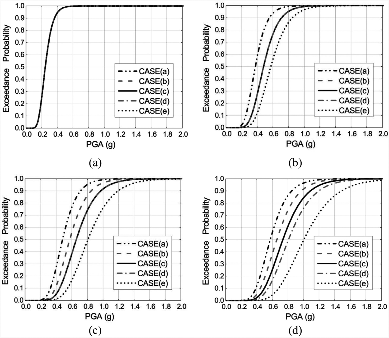
Influence of displacement capacities of fixed bearings on damage levels of themselves (μ = 0.3): (a) exceeding intact state, (b) exceeding slight damage state, (c) exceeding moderate damage state, and (d) exceeding severe damage state.

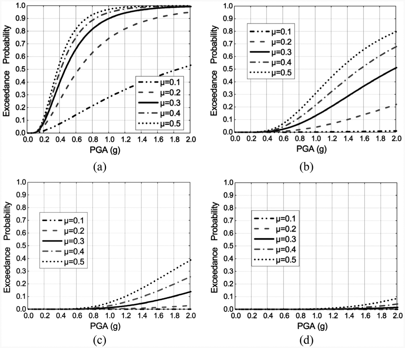
If the friction coefficients on the fixed bearings increase from 0.1 to 0.5 based on Figure 13(b), the probabilities exceeding the slight damage state of the fixed bearings change as shown in Figure 14. In Figure 14(a), a small friction coefficient on the fixed bearings implies that the relative displacement response is much larger than the displacement capacity of the fixed bearings, and the exceedance probabilities are insensitive as the relative displacement capacity changes from 4 to 8 mm. When the friction coefficient on the fixed bearings increases to a certain value, such as 0.4 and 0.5 in Figure 14(d) and (e), the exceedance probabilities become very sensitive to the relative displacement capacity, which is around the reduced relative displacement response values of the fixed bearings.

Figure 14.

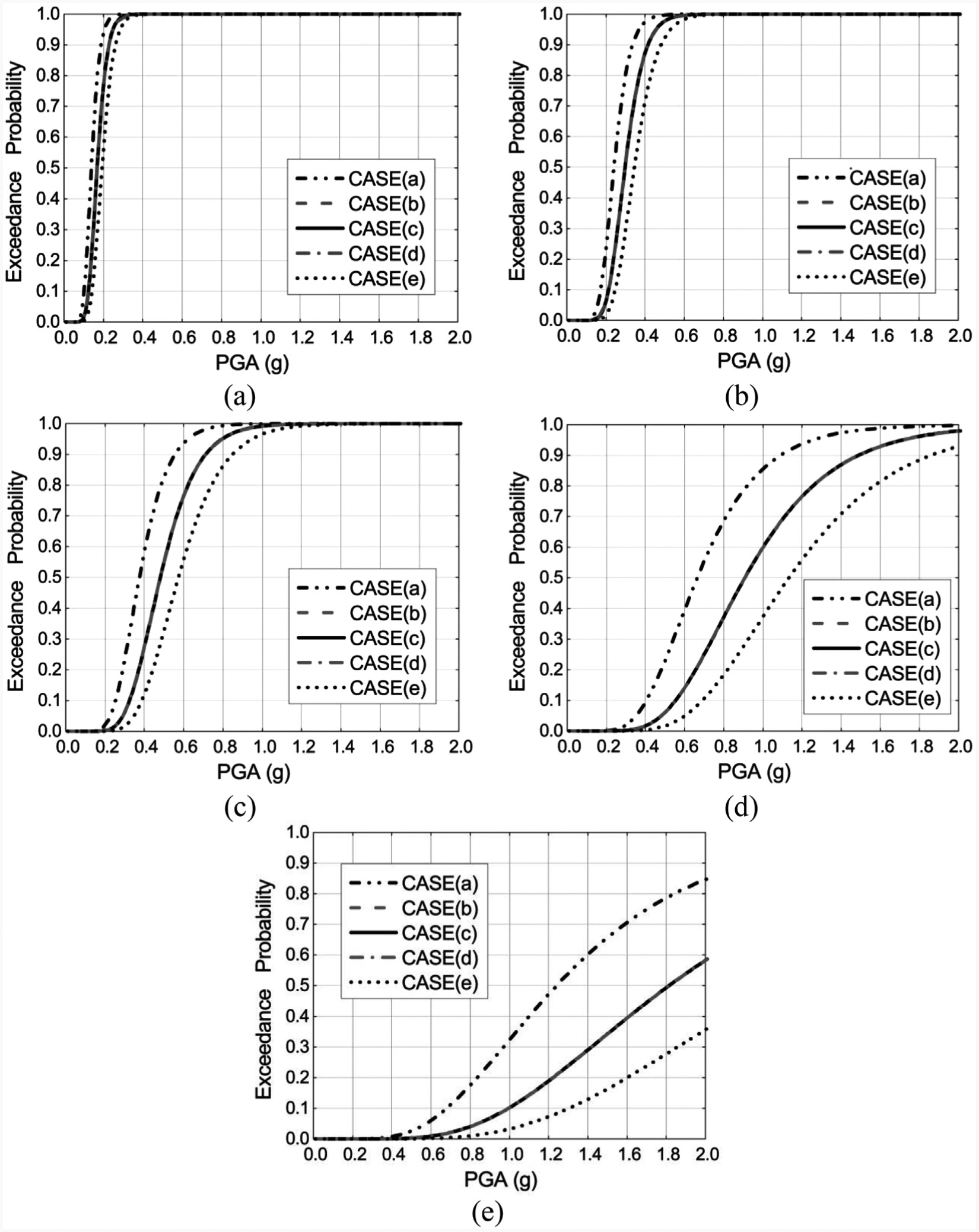
Influence of bearing displacement capacities on fragility curves for fixed bearings with various friction coefficients (exceeding slight damage state): (a) μ = 0.1, (b) μ = 0.2, (c) μ = 0.3, (d) μ = 0.4, and (e) μ = 0.5.

Conclusion

A type of friction-based fixed bearings usually changes from the un-sliding state to the sliding state during strong earthquakes, since they transfers most of the seismic force between the superstructure and the piers. The sliding friction action of those bearings acts on the seismic vulnerabilities of different components in the track–bridge system as follows:

The friction action of the friction-based fixed bearings can protect other components of the track–bridge system from severer seismic damage. This function is enlarged by decreasing the friction coefficient on the fixed bearings.

A decrease of the friction coefficient on the fixed bearings causes a larger relative displacement and a larger damage level of the fixed bearings themselves. This damage level is reduced by increasing displacement capacity of the fixed bearings.

An appropriate friction coefficient between 0.2 and 0.3 and a sufficiently large displacement capacity are almost the best combination for the fixed bearings. It protects all components of the track–bridge system from severe damage under earthquakes.

Footnotes

Declaration of Conflicting Interests

The author(s) declared no potential conflicts of interest with respect to the research, authorship, and/or publication of this article.

Funding

The author(s) disclosed receipt of the following financial support for the research, authorship, and/or publication of this article: This research is jointly supported by the National Key R&D Program of China under grant no. 2017YFB 1201204, the National Natural Science Foundations of China under grant nos 51308549 and 51378504, the Natural Science Foundations of Hunan Province under grant no. 2015JJ3159, the Special Fund of Strategic Leader in Central South University under grant no. 2016CSU001, the Innovation-driven Plan in Central South University under grant no. 2015CX006, the Experimental Foundations of the New Railway from Chengdu to Lanzhou under grant no. CLRQT-2015-010, and the Graduate Innovative Project in Central South University under grant no. 2016zzts399. The above support is greatly appreciated.

References

Chen

Jiang

Guo

et al . (2014) The seismic response of high-speed railway bridges subjected to near-fault forward directivity ground motions using a vehicle-track-bridge element. Shock and Vibration 2014: 1–17.

Choi

DesRoches

Nielson

(2004) Seismic fragility of typical bridges in moderate seismic zones. Engineering Structures 26(2): 187–199.

Cornell

Jalayer

Hamburger

et al . (2002) Probabilistic basis for 2000 SAC federal emergency management agency steel moment frame guidelines. Journal of Structural Engineering: ASCE 128(4): 526–533.

Dai

Liu

(2013) Applicability of small resistance fastener on long-span continuous bridges of high-speed railway. Journal of Central South University 20(5): 1426–1433.

Xia

(2012) Dynamic interaction of bridge–train system under non-uniform seismic ground motion. Earthquake Engineering & Structural Dynamics 41(1): 139–157.

Zou

et al . (2017) Recent developments of high-speed railway bridges in China. Structure and Infrastructure Engineering. Epub ahead of print 28 March. DOI: 10.1080/15732479.2017.1304429.

Hwang

Jernigan

Lin

Y-W

(2000) Evaluation of seismic damage to Memphis bridges and highway systems. Journal of Bridge Engineering 5(4): 322–330.

(2013) Improvement of bridge structures to increase the safety of moving trains during earthquakes. Engineering Structures 56: 501–508.

Karim

Yamazaki

(2001) Effect of earthquake ground motions on fragility curves of highway bridge piers based on numerical simulation. Earthquake Engineering & Structural Dynamics 30(12): 1839–1856.

10.

Karim

Yamazaki

(2003) A simplified method of constructing fragility curves for highway bridges. Earthquake Engineering & Structural Dynamics 32(10): 1603–1626.

11.

Kim

Mha

Lee

(2006) Effects of bearing damage upon seismic behaviors of a multi-span girder bridge. Engineering Structures 28(7): 1071–1080.

12.

Kowalsky

(2002) A displacement-based approach for the seismic design of continuous concrete bridges. Earthquake Engineering & Structural Dynamics 31(3): 719–747.

13.

Mander

Kim

Chen

et al . (1996) Response of steel bridge bearings to reversed cyclic loading. NCEER technical report 96-0014, 13 November. Buffalo, NY: National Center for Earthquake Engineering Research.

14.

Nielson

DesRoches

(2007) Seismic fragility methodology for highway bridges using a component level approach. Earthquake Engineering & Structural Dynamics 36(6): 823–839.

15.

Padgett

DesRoches

(2008) Methodology for the development of analytical fragility curves for retrofitted bridges. Earthquake Engineering & Structural Dynamics 37(8): 1157–1174.

16.

Pan

Agrawal

Ghosn

et al . (2010) Seismic fragility of multispan simply supported steel highway bridges in New York state. II: fragility analysis, fragility curves, and fragility surfaces. Journal of Bridge Engineering 15(5): 462–472.

17.

Park

Ang

(1985) Mechanistic seismic damage model for reinforced concrete. Journal of Structural Engineering: ASCE 4(111): 722–739.

18.

Ramadan

OMO

Mehanny

SSF

Elhowary

(2015) Seismic vulnerability of box girder continuous bridges under spatially variable ground motions. Bulletin of Earthquake Engineering 13(6): 1727–1748.

19.

Randall

Saiidi

Maragakis

et al . (1999) Restrainer design procedures for multi-span simply-supported bridges. MCEER technical report 99-0011, 20 July. Buffalo, NY: MCEER.

20.

Shinozuka

Feng

Kim

et al . (2000a) Nonlinear static procedure for fragility curve development. Journal of Engineering Mechanics: ASCE 126(12): 1287–1295.

21.

Shinozuka

Feng

Lee

et al . (2000b) Statistical analysis of fragility curves. Journal of Engineering Mechanics: ASCE 126(12): 1224–1231.

22.

Steelman

Filipov

Fahnestock

et al . (2014) Experimental behavior of steel fixed bearings and implications for seismic bridge response. Journal of Bridge Engineering 19: A4014007.

23.

Taskari

Sextos

(2015) Multi-angle, multi-damage fragility curves for seismic assessment of bridges. Earthquake Engineering & Structural Dynamics 44(13): 2281–2301.

24.

Vamvatsikos

Cornell

(2002) Incremental dynamic analysis. Earthquake Engineering & Structural Dynamics 31(3): 491–514.

25.

Vamvatsikos

Cornell

(2005) Developing efficient scalar and vector intensity measures for IDA capacity estimation by incorporating elastic spectral shape information. Earthquake Engineering & Structural Dynamics 34(13): 1573–1600.

26.

Wei

Wang

Liu

et al . (2016) The impact of the concave distribution of rolling friction coefficient on the seismic isolation performance of a spring-rolling system. International Journal of Non-Linear Mechanics 83(1): 65–77.

27.

Wei

Wang

Yang

et al . (2017) Seismic response of rolling isolation systems with concave friction distribution. Journal of Earthquake Engineering 21(2): 325–342.

28.

Wei

Yang

Jiang

(2015) Influence of friction variability on isolation performance of a rolling-damper isolation system. Journal of Vibroengineering 17(2): 792–801.

29.

(2015) Seismic vulnerability analysis for prestressed concrete continuous girder bridge in high-speed railway. Master Dissertation, Central South University, China (in Chinese).

30.

Zeng

Zhao

et al . (2015) Random vibration analysis of train–bridge under track irregularities and traveling seismic waves using train–slab track–bridge interaction model. Journal of Sound and Vibration 342: 22–43.

31.

Zhang

(2015) Loading-history-based track–bridge interaction analysis with experimental fastener resistance. Engineering Structures 83: 62–73.