New analytical method for determining the load-carrying capacity of two-way simply supported concrete slabs

Abstract

This article proposes the use of steel strain difference to analyse the tensile membrane action regions of two-way concrete slabs with relation to deflection while accounting for two failure criteria. The maximum load-bearing capacities and ultimate deflections of two-way slabs are subsequently determined. The proposed approach is compared with other theoretical methods and a numerical model of horizontally unrestrained concrete slabs presented by different authors. The rationality of the proposed method is validated through satisfactory comparison with results from experiments and numerical simulations.

Keywords

failure criteria load–deflection curve reinforced concrete slabs strain tensile membrane action

Introduction

In recent years, the tensile membrane action of reinforced concrete slabs under large displacements has been investigated by many researchers. The existing research has been advanced by two approaches. (1) The use of numerical models, such as the finite element method, to simulate the structural behaviour of two-way reinforced concrete slabs (Huang et al., 2003a, 2003b; Wang et al., 2013). The use of finite element-based models to analyse concrete slabs is fairly involved and relatively complex, but they are currently the most accurate tools for predicting the load–deflection response of RC slabs, as these models can incorporate both geometric and material nonlinearities. (2) The use of simple theoretical methods that consider tensile membrane action, several of which have been proposed to determine the load-carrying capacities of two-way slabs (Bailey and Toh, 2007, 2010; Burgess, 2017; Cameron and Usmani, 2005; Dong and Fang, 2010; Herraiz and Vogel, 2016; Li et al., 2007; Omer et al., 2010; Wang et al., 2015). Unlike finite element models, these methods can be easily applied in the engineering design process.

Cameron and Usmani (2005) analysed the membrane action of restrained concrete slabs based on differential equations that described slabs with large deflections. However, for design purposes, a simply supported boundary condition can be assumed in the analytical model. Thus, Bailey and Toh (2007) proposed two failure criteria to predict the ultimate loads of unrestrained concrete slabs considering tensile membrane action. However, this simple method is based on rigid, plastic behaviour as the geometry of the slab changes and thus can only predict a linear relationship between the load and deflection. Additionally, the failure criteria proposed by Bailey and Toh (2007) lead to significant underestimation of the ultimate deflections and the corresponding load-bearing capacities (Herraiz and Vogel, 2016).

Li et al. (2007) presented a new theoretical method for analysis of the limit load-bearing capacities of slabs based on a reinforcing steel failure criterion. However, the vertical shear forces along the yield line are not reasonably considered in Li’s method, and thus, the limit load-bearing capacity is not equal between each component. Additionally, this method can predict neither the occurrence of the concrete compressive crushing at the slab corners nor the nonlinear load–deflection curves of the slabs in the membrane stage.

Dong and Fang (2010) proposed a new analytical method for determining the ultimate loads of two-way reinforced concrete slabs based on the segment equilibrium method. In addition, Omer et al. (2010) proposed an energy-based, bond strength–dependent method for determining the limit loads of concrete slabs. Similarly, the load–deflection relationship predicted by Dong and Fang (2010) and Omer et al. (2010) during the membrane action stage is linear.

Herraiz and Vogel (2016) developed a new approach based on equilibrium and kinematics in which two failure criteria are used to determine the load–deflection curves of the concrete slabs. In addition, Burgess (2017) provided a systematic derivation of a new analytical approach to the tensile membrane action of lightly reinforced concrete slabs at large deflections. However, similar to the above methods, the enhancement factor tends to linearly increase with the deflection during the membrane action stage.

In fact, there are two main reasons for the linear load–deflection relationship obtained from the above methods. On one hand, most of the existing methods are based on the unchanged conventional yield-line failure mode. On the other hand, due to the unchanged failure mode, the variation of the tensile membrane action region cannot be predicted, and thus, the linear relationship between loads and deflections can be deduced. However, many experimental results have shown that the load–deflection relationships are nonlinear during the later stage, that is, the structural stiffness gradually decreases with increasing deflection. Hence, new methods should be developed to predict more reasonable load–deflection curves and two failure modes.

In this article, a new method based on steel strain difference is established to predict the load–deflection curves of concrete slabs during the tensile membrane action stage. The concrete slab is divided into five parts: the edges are defined as four rigid plates, and the centre region is assumed to be rectangular (or square). Failure criteria based on steel deformation and concrete strain are proposed to determine the limit loads and ultimate displacements of the concrete slabs. Finally, the proposed approach is compared with other methods and numerical models using full-scale and small-scale unrestrained slab tests conducted by various authors (An, 2017; Bailey and Toh, 2007; Ghoneim and McGregor, 1994; Taylor et al., 1966; Zhang et al., 2017). Overall, compared to the existing methods, the present method can more reasonably predict load–deflection curves during the membrane action stage and failure modes of the concrete slabs at the ultimate limit state.

Proposed method

Assumptions

The assumptions adopted in this approach are summarized as follows:

The slab is square or rectangular in plan, and the ratio between the length and width is not greater than two.

A slab can be divided into five parts defined by its yield lines: four exterior rigid plates and a central membrane region. For a rectangular slab, the central region is rectangular, and for a square slab, it is square.

The relationship between the angle of the surrounding rigid plates and the steel strain difference (in the central tensile membrane action region) is proposed to predict the load–deflection curves of concrete slabs.

Two failure criteria, based on steel deformation related to ultimate strain and concrete crushing strain, are established to determine the ultimate loads and displacements of concrete slabs.

Steel hardening and the bond between the concrete and reinforcement are not considered.

Vertical shear forces of the concrete slabs are considered based on the three centralized shear forces.

Initial angle

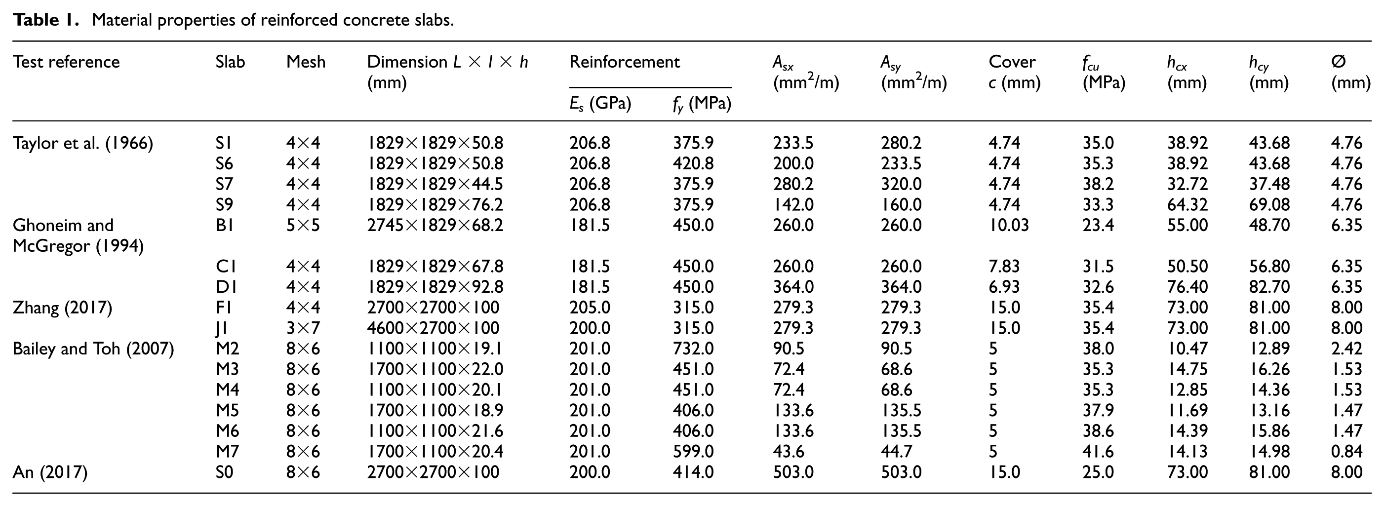
As shown in Table 1, 16 concrete slabs are used in this article because they are widely accepted to validate new methods (Bailey, 2001; Dong and Fang, 2010; Herraiz, 2016; Huang et al., 2003b; Wang et al., 2013, 2015). Apart from that of Slab S9, the angles (θ_x) of tested concrete slabs at the yield-line loads were between 0.02 and 0.08 rad, as shown in Table 2. Based on the Herraiz and Vogel (2016) method, the average angle of deflection of each slab corresponding to its yield-line load is approximately 0.05 rad. Therefore, when the tensile membrane action of the slab begins to develop, its initial angle (θ_x,₀) is assumed to be 0.05 rad in this article. In addition, the yield-line load of each slab is calculated based on the conventional yield-line method.

Table 1.

Material properties of reinforced concrete slabs.

Test reference	Slab	Mesh	Dimension L × l × h (mm)	Reinforcement		A_sx (mm²/m)	A_sy (mm²/m)	Cover c (mm)	f_cu (MPa)	h_cx (mm)	h_cy (mm)	Ø (mm)
				E_s (GPa)	f_y (MPa)
Taylor et al. (1966)	S1	4×4	1829×1829×50.8	206.8	375.9	233.5	280.2	4.74	35.0	38.92	43.68	4.76
	S6	4×4	1829×1829×50.8	206.8	420.8	200.0	233.5	4.74	35.3	38.92	43.68	4.76
	S7	4×4	1829×1829×44.5	206.8	375.9	280.2	320.0	4.74	38.2	32.72	37.48	4.76
	S9	4×4	1829×1829×76.2	206.8	375.9	142.0	160.0	4.74	33.3	64.32	69.08	4.76
Ghoneim and McGregor (1994)	B1	5×5	2745×1829×68.2	181.5	450.0	260.0	260.0	10.03	23.4	55.00	48.70	6.35
	C1	4×4	1829×1829×67.8	181.5	450.0	260.0	260.0	7.83	31.5	50.50	56.80	6.35
	D1	4×4	1829×1829×92.8	181.5	450.0	364.0	364.0	6.93	32.6	76.40	82.70	6.35
Zhang (2017)	F1	4×4	2700×2700×100	205.0	315.0	279.3	279.3	15.0	35.4	73.00	81.00	8.00
	J1	3×7	4600×2700×100	200.0	315.0	279.3	279.3	15.0	35.4	73.00	81.00	8.00
Bailey and Toh (2007)	M2	8×6	1100×1100×19.1	201.0	732.0	90.5	90.5	5	38.0	10.47	12.89	2.42
	M3	8×6	1700×1100×22.0	201.0	451.0	72.4	68.6	5	35.3	14.75	16.26	1.53
	M4	8×6	1100×1100×20.1	201.0	451.0	72.4	68.6	5	35.3	12.85	14.36	1.53
	M5	8×6	1700×1100×18.9	201.0	406.0	133.6	135.5	5	37.9	11.69	13.16	1.47
	M6	8×6	1100×1100×21.6	201.0	406.0	133.6	135.5	5	38.6	14.39	15.86	1.47
	M7	8×6	1700×1100×20.4	201.0	599.0	43.6	44.7	5	41.6	14.13	14.98	0.84
An (2017)	S0	8×6	2700×2700×100	200.0	414.0	503.0	503.0	15.0	25.0	73.00	81.00	8.00

Table 2.

Initial deflection angle and steel strain difference of concrete slabs.

Parameter	Slab
	S1	S6	S7	S9	B1	C1	D1	F1	J1	M2	M3	M4	M5	M6	M7	S0
θ_x,₀^a (10⁻²)	5	2	3	0.1	4	4	3	2	6	7	5	4	8	5	4	2
θ_x,₀^b (10⁻²)	5	5	4	7	6	6	9	6	6	2	3	2	2	3	3	6
$Δ {\bar{ε}}_{sx, 0}$ (10⁻⁵)	2.4	3.0	4.7	2.8	2.8	6.6	11.7	0.9	0.5	10.6	1.0	0.9	1.1	11.6	0.8	0.5
$Δ {\bar{ε}}_{sx, 1}$ (10⁻⁴)	18.1	24.4	29.1	15.3	19.8	24.0	20.6	5.8	22.8	23.5	26.1	27.8	34.4	36.8	16.6	5.2

$Δ {\bar{ε}}_{sx, 0}$ : at the conventional yield-line load; $Δ {\bar{ε}}_{sx, 1}$ : at the limit load.

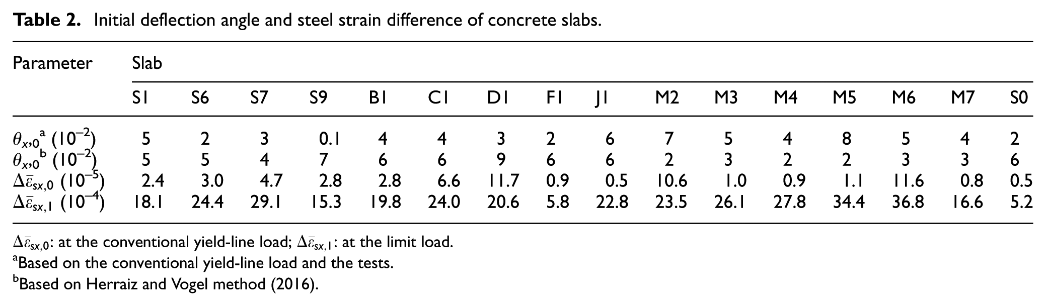
Based on the conventional yield-line load and the tests.

Based on Herraiz and Vogel method (2016).

On one hand, θ_x,₀ is characterized by the beginning of the tensile membrane action in the concrete slab. However, there is no doubt that for one slab, θ_x,₀ may be dependent on several factors, such as the steel ratio and slenderness ratio. Hence, an accurate analytical method should be established to obtain a reasonable value. On the other hand, θ_x,₀ is mainly used to establish the relationship between the angle and steel strain difference, as discussed later.

Analytical mode

According to experimental observations (An, 2017; Bailey and Toh, 2007), through-depth tensile cracks of the concrete in a two-way slab often occur at the cross-sections. As a result of these through-depth cracks, the deflection model shown in Figure 1(a) and (b) is adopted, in which the deflection of the face of the central region (⑤) under membrane action is approximated as a rectangular paraboloid, while Plates ①–④ are assumed to be rigid. The force distribution in the slab during the membrane action stage is approximated, as shown in Figure 1(c).

Figure 1.

Analytical model considering tensile membrane action. (a) Division of the slab and coordinates of plates. (b) Diagram of plate deflection (one quarter slab). (c) In-plane force distribution.

Model parameters

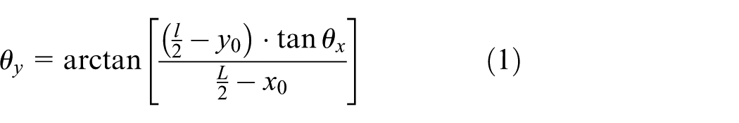
Determination of θ_y

According to geometric compatibility (Figure 1(b)), θ_y can be expressed as

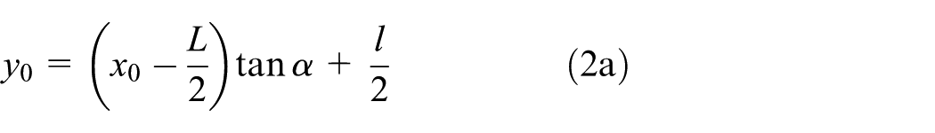
θ_{y} = \arctan [\frac{(\frac{l}{2} - y_{0}) \cdot \tan θ_{x}}{\frac{L}{2} - x_{0}}]

(1)

Determination of x₀ and y₀

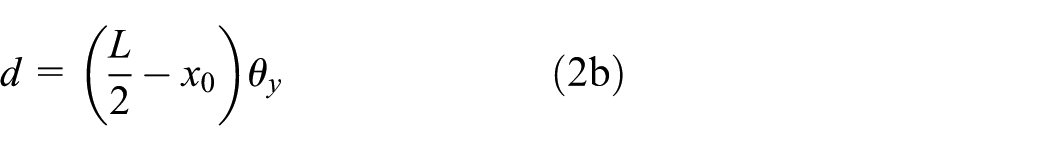
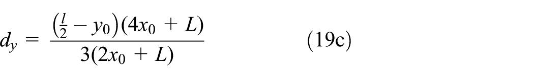
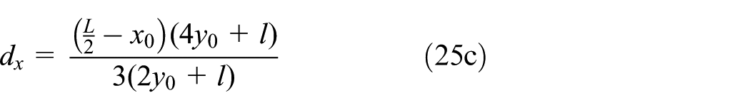
According to Figure 1(a) and (b), y₀ and d can be defined as

y_{0} = (x_{0} - \frac{L}{2}) \tan α + \frac{l}{2}

(2a)

d = (\frac{L}{2} - x_{0}) θ_{y}

(2b)

As shown in Figures 1(a) and 2, by the relationship of Point D (x₀, 0) and the angle (θ_y), the equation of line Z_DE can be defined as

z_{DE} = - \tan θ_{y} \cdot x + x_{0} \cdot \tan θ_{y}

(3)

Figure 2.

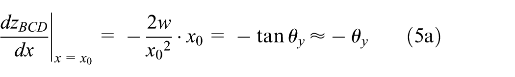
Cross-section of the slab parallel to the x direction (left), and strains ${\bar{ε}}_{mid, sx}$ and ${\bar{ε}}_{edge, sx}$ parallel to the x direction (right).

Using Points C (0, w) and D (x₀, 0), the equation of the parabolic line Z_BCD (in the x direction) can be determined as follows

z_{BCD} = (- \frac{x^{2}}{x_{0}^{2}} + 1) w

(4)

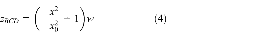
Therefore, according to equations (3) and (4) and assuming the same slope at the intersection of the yield-line and central region, x₀ can be obtained by

{\frac{d z_{BCD}}{dx} |}_{x = x_{0}} = - \frac{2 w}{{x_{0}}^{2}} \cdot x_{0} = - \tan θ_{y} \approx - θ_{y}

(5a)

x_{0} = \frac{2 w}{θ_{y}}

(5b)

Steel strain difference

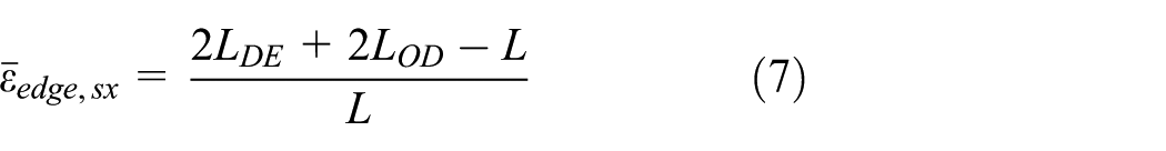
As shown in Figure 2, the parabolic line Z_BCD is replaced by two diagonal chords (L_BC and L_CD), meaning that the average strain in the reinforcing steel at mid-span can be expressed as

{\bar{ε}}_{mid, sx} = \frac{2 L_{DE} + 2 L_{CD} - L}{L}

(6)

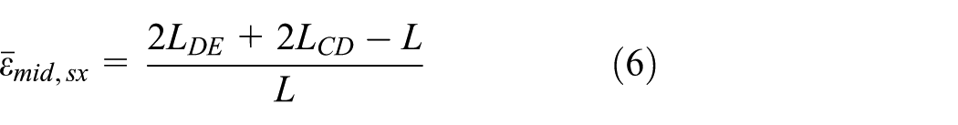
where L_DE is the length of rigid Plate ① or ②; L_CD is the length of the central region.

In a similar manner, the average strain ${\bar{ε}}_{edge, sx}$ in the steel (Figure 2) at the edges of the rectangular paraboloid can be expressed as

{\bar{ε}}_{edge, sx} = \frac{2 L_{DE} + 2 L_{OD} - L}{L}

(7)

where L_OD (= L_OB) is the length of the reinforcement at the edge of the rectangular paraboloid, that is, x₀, as indicated in Figure 1(b).

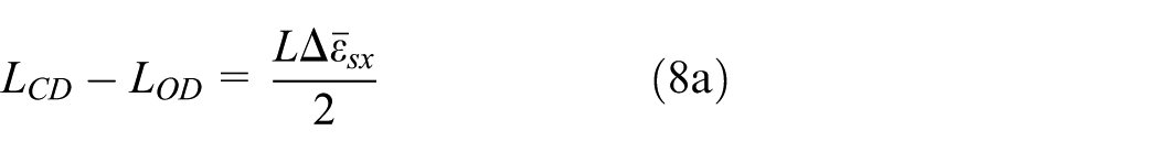
Using equations (6) and (7), the following equations can be obtained

L_{CD} - L_{OD} = \frac{L Δ {\bar{ε}}_{sx}}{2}

(8a)

Δ {\bar{ε}}_{sx} = {\bar{ε}}_{mid, sx} - {\bar{ε}}_{edge, sx}

(8b)

L_{OD} = x_{0}, L_{CD} = \sqrt{x_{0}^{2} + w^{2}}

(8c)

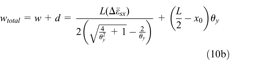
According to equations (5b) and (8a) to (8c), w can be obtained by

w = \frac{L Δ {\bar{ε}}_{sx}}{2 (\sqrt{\frac{4}{θ_{y}^{2}} + 1} - \frac{2}{θ_{y}})}

(9)

Thus, according to equations (2b) and (9), the mid-span deflection ( $w_{total}$ ) of the slab can be defined as

w_{total} = w + d

(10a)

w_{total} = w + d = \frac{L (Δ {\bar{ε}}_{sx})}{2 (\sqrt{\frac{4}{θ_{y}^{2}} + 1} - \frac{2}{θ_{y}})} + (\frac{L}{2} - x_{0}) θ_{y}

(10b)

Angle–steel strain difference relationship

According to equations (1), (2a), (5b) and (9), the relationship between the angle (θ_x) and the steel strain difference ( $Δ {\bar{ε}}_{sx}$ ) has a considerable effect on the tensile membrane action region (x₀ and y₀) of the slab. According to equation (9), $Δ {\bar{ε}}_{sx}$ tends to nonlinearly increase with the angle θ_y (or θ_x). This leads to the nonlinear increase of x₀ and y₀ with an increase in deflection or angle.

However, as the slab approaches the limit state, the tensile membrane action region (x₀ and y₀) does not change significantly because the complete membrane net is almost completely developed (Herraiz and Vogel, 2016). Therefore, the values of x₀ and y₀ (defining the tensile membrane action region) for a slab in the later stages of loading can be assumed to be constant. This implies that a linear relationship between the deflection (w) and the angle (θ_y) can be obtained using equation (5b). Experimental results in the literature (An, 2017) have verified this assumption, that is, a central crack region on the bottom surface of Slab S0 remained basically unchanged in the later loading stages, and the width of several main cracks gradually increased until the ultimate limit mid-span deflection was reached. It is interesting to note that with the increasing deflection of the slab, the linear relationship between the angle (θ_x) and steel strain difference ( $Δ {\bar{ε}}_{sx}$ ) accurately reflects the behaviour of the slab, as discussed later.

According to the numerical analysis, the steel strain difference between concrete slabs at their yield-line loads and those at their limit state can be calculated, as indicated in Table 2. The numerical method of the steel strain difference will be discussed later. Because this approach requires neglecting a number of uncertain parameters and complex interactions between concrete and steel, $Δ {\bar{ε}}_{sx, 0}$ and $Δ {\bar{ε}}_{sx, 1}$ are established as 1.0×10⁻⁵ and 8×10⁻⁴ in this article, with corresponding angles of 0.05 rad (θ_x,₀) and 0.15 rad (θ_x,₁), respectively. Meanwhile, θ_x,₀ is determined based on the experimental results (Table 2), and θ_x,₁ is determined according to the reference (Li et al., 2007).

The linear relationship between $Δ {\bar{ε}}_{sx}$ and θ_x is defined as

Δ {\bar{ε}}_{sx} = \frac{Δ {\bar{ε}}_{sx, 1} - Δ {\bar{ε}}_{sx, 0}}{θ_{x, 1} - θ_{x, 0}} θ_{x} + \frac{Δ {\bar{ε}}_{sx, 0} \times θ_{x, 1} - Δ {\bar{ε}}_{sx, 1} \times θ_{x, 0}}{θ_{x, 1} - θ_{x, 0}}

(11)

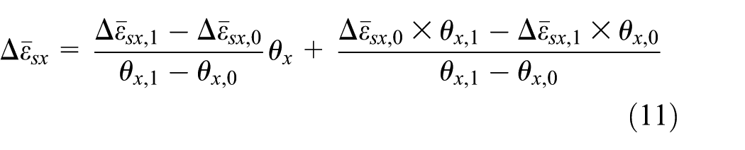
Due to a lack of experimental data (steel strains), the relationship between the angle and steel strain difference was established based on numerical analysis, and the numerical model was validated by a good correspondence between the predicted and measured bottom steel strain of Slab D1 (Ghoneim and McGregor, 1994), as shown in Figure 3. Thus, taking Slabs B1, C1 and D1 as examples, Figure 3 indicates that the relationship between the angle θ_x (rigid plate) and the steel strain difference $Δ {\bar{ε}}_{sx}$ (membrane action region) is basically linear. Because of the neglect of the effect of other factors (bond–slip and local cracks), the present steel strain difference (equation (11)) tends to be lower than the numerical results.

Figure 3.

Comparison of the predicted and measured load–strain of the mid-span bottom steel in Slab D1 (left), numerical result and proposed steel strain difference angle model of Slabs B1, C1 and D1 (right).

Using equations (1), (5b), (10b) and (11), the function for states between x₀ and $Δ {\bar{ε}}_{sx}$ can be easily obtained. As the steel strain difference increases, x₀ and y₀ (which define the membrane region) gradually increase until their peak values are reached. Note that x₀ and y₀ retain their peak values as the subsequent angle θ_x increases. In this case, according to equations (1) and (5b), the value (2w/θ_y) remains constant until one failure criterion of the slab is reached. In all, if θ_x is given, x₀ and y₀ can be obtained using the above equations.

Equilibrium equations

Internal force equilibrium equations

As shown in Figure 4(a) and (b), at the intersection of the central region and the rigid plates, the tension forces in the x and y direction reinforcement (T_x and T_y) can be decomposed into horizontal (T_xh and T_yh) and vertical components (T_xv and T_yv).

Figure 4.

Diagram of the forces in rigid Plates ①–④ and central Region ⑤ of the slab. (a) Diagram of forces in rigid Plate ① or ②. (b) Diagram of forces in rigid Plate ③ or ④. (c) Diagram of forces in the central Region ⑤.

According to Figure 1(b) and equation (5b), for the x direction reinforcement, $φ_{x}$ can be obtained by

φ_{x} = \arctan (\frac{w}{x_{0}}) = \arctan \frac{θ_{y}}{2}

(12)

Thus

\sin φ_{x} \approx \frac{θ_{y}}{2}

(13a)

\cos φ_{x} = \sqrt{1 - \frac{θ_{y}^{2}}{4}}

(13b)

The horizontal and vertical forces in the x direction reinforcement are

T_{xh} = T_{x} \cdot \cos φ_{x} = T_{x} \cdot \sqrt{1 - \frac{θ_{y}^{2}}{4}}

(14a)

T_{xv} = T_{x} \cdot \sin φ_{x} = T_{x} \cdot \frac{θ_{y}}{2}

(14b)

T_{x} = f_{y} \cdot A_{sx}

(14c)

According to Figure 1(b), for the y direction reinforcement, $φ_{y}$ can be obtained by

φ_{y} = \arctan \frac{w}{y_{0}}

(15)

The vertical and horizontal component forces in the reinforcement parallel to the y direction are given by

T_{yh} = T_{y} \cdot \cos φ_{y}

(16a)

T_{yv} = T_{y} \cdot \sin φ_{y}

(16b)

T_{y} = f_{y} \cdot A_{sy}

(16c)

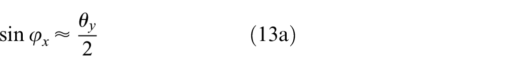
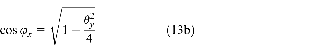
In this article, φ_x (φ_y) is the angle of x (y) direction steels at the edge of the tensile membrane region and increases with deflection. As discussed above, φ_x (φ_y) is used to get the horizontal and vertical components of x (y) direction steel forces at a certain deflection. In fact, the variation of φ_x (φ_y) also indicates that x (y) direction steels extend, and that the steel strain difference develops.

According to Figure 1(c), the equilibrium equations for in-plane forces in the x and y directions are

2 C \cdot \sin α = 2 S \cdot \cos α + 2 y_{0} T_{xh}

(17a)

2 C \cdot \cos α + 2 S \cdot \sin α = 2 x_{0} T_{yh}

(17b)

As a result, C and S can be calculated using equations (17a) and (17b) such that

C = x_{0} T_{yh} \cdot \cos α + y_{0} T_{xh} \cdot \sin α

(18a)

S = x_{0} T_{yh} \cdot \sin α - y_{0} T_{xh} \cdot \cos α

(18b)

Equilibrium equations of different regions

For rigid Plates ①–④, the bending equilibrium equations about the support O (or O′) can be determined according to Figure 4(a) and (b).

1. Bending equilibrium equations for rigid Plate ① or ②

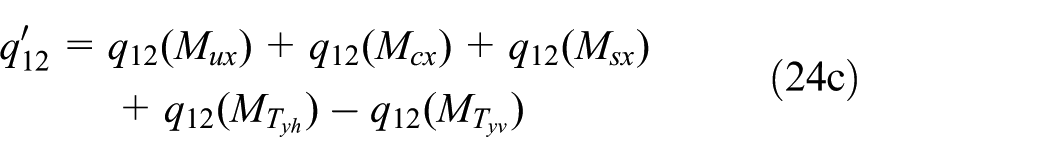
As shown in Figure 4(a), the bending moment due to the vertical uniform load (q₁₂) on rigid Plate ① or ② is defined as

M_{q 12} = q_{12} \cdot A_{12} \cdot d_{y}

(19a)

A_{12} = \frac{(2 x_{0} + L) (\frac{l}{2} - y_{0})}{2}

(19b)

d_{y} = \frac{(\frac{l}{2} - y_{0}) (4 x_{0} + L)}{3 (2 x_{0} + L)}

(19c)

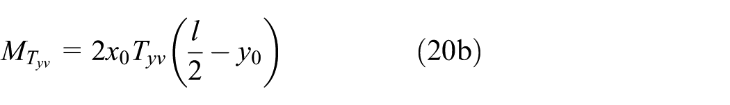
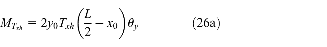
The bending moment due to the horizontal (T_yh) and vertical components (T_yv) of the force in the reinforcement parallel to the y direction is defined as

M_{T_{yh}} = 2 x_{0} T_{yh} (\frac{l}{2} - y_{0}) θ_{x}

(20a)

M_{T_{yv}} = 2 x_{0} T_{yv} (\frac{l}{2} - y_{0})

(20b)

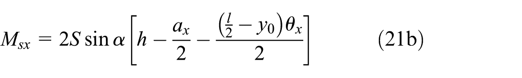
As shown in Figure 4(a), for rigid Plate ① or ②, the bending moment about the support O induced by the compression force (C) and the shear force (S) can be expressed as

M_{cx} = 2 C \cos α [h - \frac{a_{x}}{2} - \frac{(\frac{l}{2} - y_{0}) θ_{x}}{3}]

(21a)

M_{sx} = 2 S \sin α [h - \frac{a_{x}}{2} - \frac{(\frac{l}{2} - y_{0}) θ_{x}}{2}]

(21b)

a_{x} = C / [f_{c} \cdot (L / 2 - x_{0}) / \cos α]

(21c)

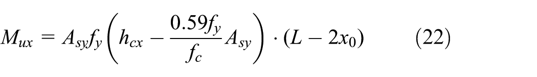
In addition, the bending resistance about the yield line parallel to the x direction can be determined by (Bailey and Toh, 2007)

M_{ux} = A_{sy} f_{y} (h_{cx} - \frac{0.59 f_{y}}{f_{c}} A_{sy}) \cdot (L - 2 x_{0})

(22)

In this article, the vertical shear forces acting along the yield lines were considered. This is accomplished by replacing the actual shear forces acting directly along the yield lines with two statically equivalent nodal forces, as indicated in Figure 1(c). Therefore, the moment about the support O due to the vertical shear forces (Q₁) of Plate ① can be determined by

M_{Q_{1}} = 2 Q_{1} \cdot (l / 2 - y_{0})

(23)

According to equations (19a), (20a), (20b), (21a), (21b), (22) and (23), the bending moment equilibrium equation for rigid Plate ① or ② about the support O can be obtained by

M_{q 12} + M_{T_{yv}} - M_{T_{yh}} - M_{cx} - M_{sx} - M_{ux} \mp M_{Q_{1}} = 0

(24a)

\begin{array}{l} q_{12} = (M_{u x} + M_{c x} + M_{s x} + M_{T_{y h}} - M_{T_{y v}} \pm M_{Q_{1}}) / (A_{12} \times d_{12}) \\ = {q'}_{12} \pm q_{12} (M_{Q_{1}}) \end{array}

(24b)

\begin{array}{l} {q'}_{12} = q_{12} (M_{u x}) + q_{12} (M_{c x}) + q_{12} (M_{s x}) \\ + q_{12} (M_{T_{y h}}) - q_{12} (M_{T_{y v}}) \end{array}

(24c)

2. Bending equilibrium equations for Plate ③ or ④

As shown in Figure 4(b), the bending moment due to the vertical uniform load q₃₄ on the plate is defined by

M_{q 34} = q_{34} \cdot A_{34} \cdot d_{x}

(25a)

A_{34} = \frac{(2 y_{0} + l) (\frac{L}{2} - x_{0})}{2}

(25b)

d_{x} = \frac{(\frac{L}{2} - x_{0}) (4 y_{0} + l)}{3 (2 y_{0} + l)}

(25c)

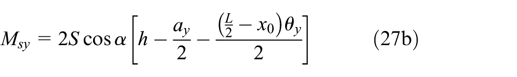
The bending moment due to the horizontal and vertical components (T_xh and T_xv) of the reinforcement force is calculated by

M_{T_{xh}} = 2 y_{0} T_{xh} (\frac{L}{2} - x_{0}) θ_{y}

(26a)

M_{T_{xv}} = 2 y_{0} T_{xv} (\frac{L}{2} - x_{0})

(26b)

For Plate ③ or ④, the bending moment about the support O′ induced by C and S can be expressed as

M_{cy} = 2 C \sin α [h - \frac{a_{y}}{2} - \frac{(\frac{L}{2} - x_{0}) θ_{y}}{3}]

(27a)

M_{sy} = 2 S \cos α [h - \frac{a_{y}}{2} - \frac{(\frac{L}{2} - x_{0}) θ_{y}}{2}]

(27b)

a_{y} = C / [f_{c} \cdot (l / 2 - y_{0}) / \sin α]

(27c)

The bending resistance per unit width about the yield line parallel to the y-axis can be determined by

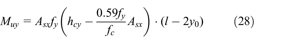
M_{uy} = A_{sx} f_{y} (h_{cy} - \frac{0.59 f_{y}}{f_{c}} A_{sx}) \cdot (l - 2 y_{0})

(28)

As indicated in Figure 1(c), the moment about the support O′ due to the vertical shear forces (Q₂) can be determined by

M_{Q_{2}} = 2 Q_{2} \cdot (L / 2 - x_{0})

(29)

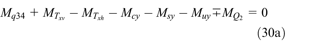
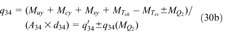
According to equations (25a), (26a), (26b), (27a), (27b), (28) and (29), the bending moment equilibrium equation for Plate ③ or ④ about the support O′ can be obtained by

M_{q 34} + M_{T_{xv}} - M_{T_{xh}} - M_{cy} - M_{sy} - M_{uy} \mp M_{Q_{2}} = 0

(30a)

\begin{array}{l} q_{34} = (M_{u y} + M_{c y} + M_{s y} + M_{T_{x h}} - M_{T_{x v}} \pm M_{Q_{2}}) / \\ (A_{34} \times d_{34}) = {q'}_{34} \pm q_{34} (M_{Q_{2}}) \end{array}

(30b)

\begin{array}{l} {q'}_{34} = q_{34} (M_{u y}) + q_{34} (M_{c y}) + q_{34} (M_{s y}) \\ + q_{34} (M_{T_{x h}}) - q_{34} (M_{T_{x v}}) \end{array}

(30c)

3. Equilibrium equation of central Region ⑤

As shown in Figure 4(c), the vertical components of the reinforcement force are

{T'}_{xv} = T_{x} \cdot \sin θ_{y}, {T'}_{yv} = T_{y} \cdot \sin θ_{x}

(31)

Clearly, equilibrium requires that the shear forces acting on either side of the yield line be equal and opposite (Figure 1(c)); thus, the following relationship is obtained

Q_{3} = - (Q_{1} + Q_{2})

(32)

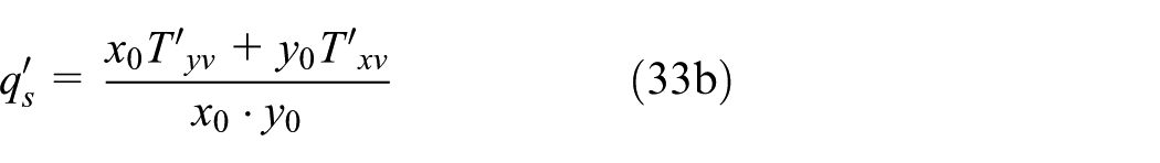
Thus, the load-bearing capacity (q_s) of the central region of the slab can be determined by

\begin{array}{l} q_{s} = \frac{4 [x_{0} {T'}_{y v} + y_{0} {T'}_{x v}] \mp 4 Q_{3}}{4 x_{0} \cdot y_{0}} \\ = \frac{x_{0} {T'}_{y v} + y_{0} {T'}_{x v} \mp Q_{3}}{x_{0} \cdot y_{0}} = {q'}_{s} \mp q_{s} (Q_{3}) \end{array}

(33a)

{q'}_{s} = \frac{x_{0} {T'}_{yv} + y_{0} {T'}_{xv}}{x_{0} \cdot y_{0}}

(33b)

Load capacity

The load-bearing capacity (equations (24b), (30b) and (33a)) must be equal along the yield lines between individual plates and thus equal to that of the entire slab as follows

q = q_{s} = q_{12} = q_{34}

(34)

Additionally, for a given load-carrying capacity (q), the corresponding total mid-span deflection (w_total) of the slab can be obtained using equation (10b). Figure 5 shows the flow chart for analysing the load–deflection curves of concrete slabs based on the above equations, and thus, an analytic solution for each slab can be obtained.

Figure 5.

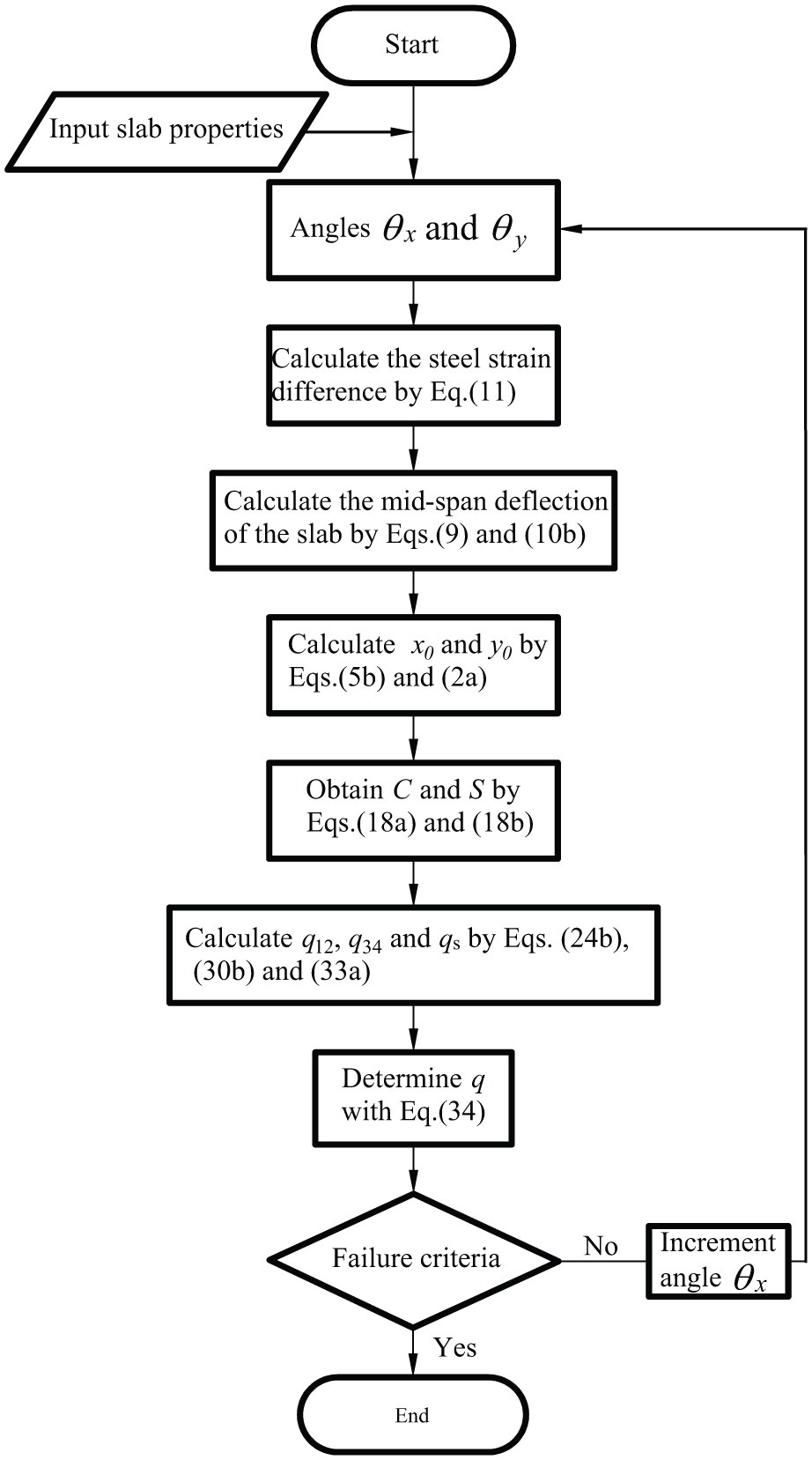
Flow chart for calculating the load-carrying capacity of concrete slabs.

Failure criteria

Compressive failure due to concrete crushing

Failure is predicted by limiting the maximum compressive strain ε_corner at the corners (on the top surface) to the ultimate compressive concrete strain ε_cu (in the range of 0.0033–0.0038) (Ye, 2005). The higher ultimate concrete strain (0.0038) was used due to higher compressive strength (small-scale slabs in Table 1), and the ultimate concrete strain of full-scale slabs with lower concrete strength was taken as 0.0035.

ε_corner is estimated assuming elastic behaviour of the concrete under the combined action of the bending moment and axial force such that

\begin{array}{l} ε_{c o r n e r} = k [\frac{C}{A E_{c}} + a_{x} \frac{M_{C}}{E_{c} I_{e f f}}] \\ = k [\frac{f_{c}}{E_{c}} + a_{x} \frac{C \times [h_{0} - (a_{x} / 2)]}{E_{c} I_{e f f}}], E_{c} = \frac{10^{11}}{2.2 + \frac{34.74}{f_{c u}}} \end{array}

(35a)

I_{eff} = \frac{I_{cr}}{2} \times (1.0 + \frac{w_{yield}}{w_{total}})

(35b)

I_{cr} = \frac{[(L / 2 - x_{0}) / \cos α] {a_{x}}^{3}}{3} + \frac{E_{s}}{E_{c}} A_{s} (h_{0} - a_{x})^{2}

(35c)

k is one modified factor. On one hand, because the concentrated force (C) is used in equation (35a), k should be 2.0 based on the triangle distribution of the compressive stresses (Figure 1(c)). Alternately, for the normal concrete (f_c: 15–40 N/mm²), the peak strain corresponding to f_c is approximately 2.0×10⁻³, its crushing strain ranges from 3.5 to 3.8 (×10⁻³) and the maximum ratio is approximately 1.9. However, for the proposed method, ε_corner was calculated based on the elastic property (i.e. E_c). Hence, to coincide with the conventional concrete crushing strain, k is further multiplied by 2.0. In all, k is assumed to be 4.0 in this article.

Reinforcement failure

To define the steel failure mode of one slab, the ultimate steel strain ε_su at mid-span must be considered, such as 0.01 (GB50010-2010, 2011). In addition, according to the reference (Bailey, 2001), the mid-span steel strain ε_s can be calculated by

ε_{s} = \frac{8 w_{total}^{2}}{3 l^{2}}

(36)

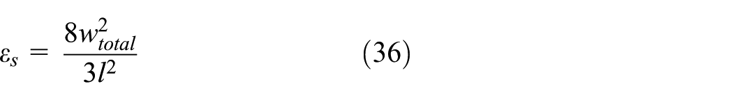
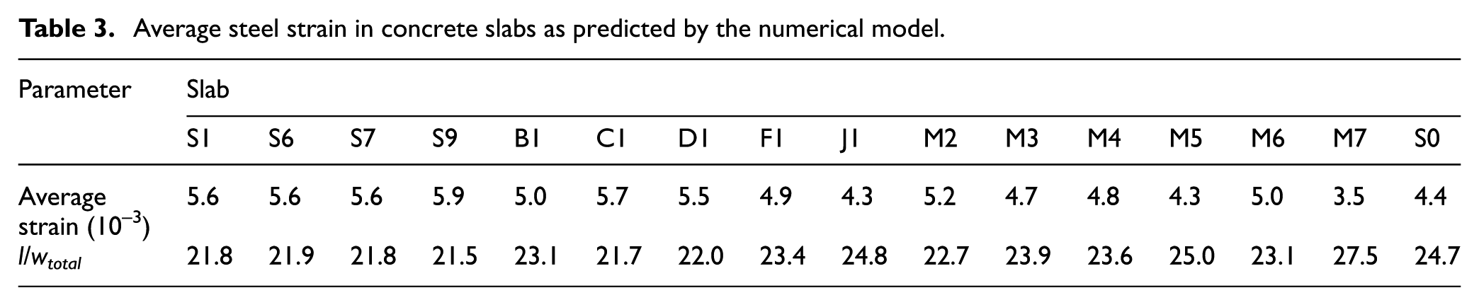
Equation (36) assumes that the strain is a uniform value along the length of the slab. According to the numerical model, as the central steel in the shorter span direction reached 0.01, the average steel strain and the average span-to-deflection ratio (l/w_total) were approximately 0.005 and 23.2, respectively, as shown in Table 3. Finally, to define the reinforcing failure mode, the limiting mid-span deflection of the slab can be determined using l/20, and this failure criterion conforms to that proposed in the references (Kodur and Dwaikat, 2008; Wang et al., 2015).

Table 3.

Average steel strain in concrete slabs as predicted by the numerical model.

Parameter	Slab
	S1	S6	S7	S9	B1	C1	D1	F1	J1	M2	M3	M4	M5	M6	M7	S0
Average strain (10⁻³)	5.6	5.6	5.6	5.9	5.0	5.7	5.5	4.9	4.3	5.2	4.7	4.8	4.3	5.0	3.5	4.4
l/w_total	21.8	21.9	21.8	21.5	23.1	21.7	22.0	23.4	24.8	22.7	23.9	23.6	25.0	23.1	27.5	24.7

Verification and discussion

Results from full-scale and small-scale concrete slab tests conducted by different authors are used for this comparison. In addition, for finite element modelling, due to the double symmetry of both support and loading conditions, only a quarter of each subject concrete slab is analysed, and the even mesh adopted for each concrete slab is shown in Table 1. The details of the nonlinear finite element model used for the validation can be found in the literature (Wang et al., 2013).

Comparison of the proposed method with experimental and other theoretical results

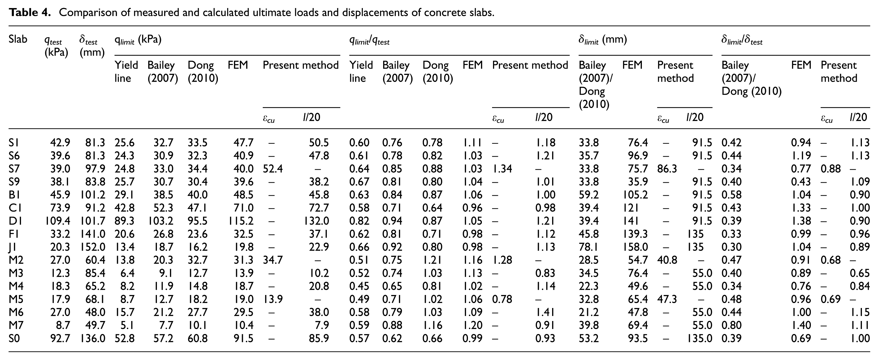
The load–deflection relationships of concrete slabs were predicted by different methods, as shown in Figure 6. Note that due to space limitations, only four slabs (Slabs B1, C1, F1 and M4) of 16 tests (Table 1) are plotted in this article. Meanwhile, considering that the values of the angle and steel strain difference were derived based on the 16 tests (Table 1), and thus, Slabs S8, S12, S18 and S20 (Herraiz, 2016) were used to further validate the rationality of the proposed method, as indicated in Figure 6. As shown in Table 4, the predictions of q_limit and δ_limit by different theories are compared against the experimental results (q_test and δ_test). The results are summarized as follows:

1. Figure 6 shows that during the membrane stage, the load–deflection curves estimated by the proposed design method agree well with the experimental results. The predictions for small-scale slabs, however, show a larger deviation from the tests due to the low flexural component of the small-scale test slabs. Because the contribution of flexural components is overestimated in the proposed methods, they assign a stiffer behaviour to the small-scale slabs than that present in reality. Additionally, the steel used in the small-scale test specimens did not exhibit a distinct yield plateau, instead exhibiting strain hardening behaviour (Bailey and Toh, 2007). Because strain hardening behaviour is considered beyond the scope of the research presented in this article, disagreements between the predicted and experimental results are to be expected.

Figure 6.

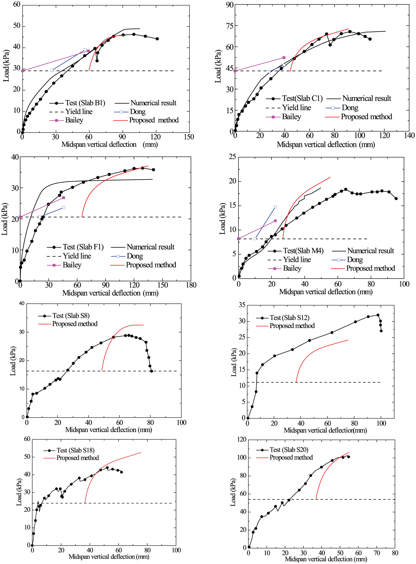
Comparison between experimental results and the load-carrying capacity of concrete slabs calculated by different methods.

Table 4.

Comparison of measured and calculated ultimate loads and displacements of concrete slabs.

Slab	q_test (kPa)	δ_test (mm)	q_limit (kPa)						q_limit/q_test						δ_limit (mm)				δ_limit/δ_test
			Yield line	Bailey (2007)	Dong (2010)	FEM	Present method		Yield line	Bailey (2007)	Dong (2010)	FEM	Present method		Bailey (2007)/Dong (2010)	FEM	Present method		Bailey (2007)/Dong (2010)	FEM	Present method
							ε_cu	l/20					ε_cu	l/20			ε_cu	l/20			ε_cu	l/20
S1	42.9	81.3	25.6	32.7	33.5	47.7	−	50.5	0.60	0.76	0.78	1.11	−	1.18	33.8	76.4	−	91.5	0.42	0.94	−	1.13
S6	39.6	81.3	24.3	30.9	32.3	40.9	−	47.8	0.61	0.78	0.82	1.03	−	1.21	35.7	96.9	−	91.5	0.44	1.19	−	1.13
S7	39.0	97.9	24.8	33.0	34.4	40.0	52.4	−	0.64	0.85	0.88	1.03	1.34	−	33.8	75.7	86.3	−	0.34	0.77	0.88	−
S9	38.1	83.8	25.7	30.7	30.4	39.6	−	38.2	0.67	0.81	0.80	1.04	−	1.01	33.8	35.9	−	91.5	0.40	0.43	−	1.09
B1	45.9	101.2	29.1	38.5	40.0	48.5	−	45.8	0.63	0.84	0.87	1.06	−	1.00	59.2	105.2	−	91.5	0.58	1.04	−	0.90
C1	73.9	91.2	42.8	52.3	47.1	71.0	−	72.7	0.58	0.71	0.64	0.96	−	0.98	39.4	121	−	91.5	0.43	1.33	−	1.00
D1	109.4	101.7	89.3	103.2	95.5	115.2	−	132.0	0.82	0.94	0.87	1.05	−	1.21	39.4	141	−	91.5	0.39	1.38	−	0.90
F1	33.2	141.0	20.6	26.8	23.6	32.5	−	37.1	0.62	0.81	0.71	0.98	−	1.12	45.8	139.3	−	135	0.33	0.99	−	0.96
J1	20.3	152.0	13.4	18.7	16.2	19.8	−	22.9	0.66	0.92	0.80	0.98	−	1.13	78.1	158.0	−	135	0.30	1.04	−	0.89
M2	27.0	60.4	13.8	20.3	32.7	31.3	34.7	−	0.51	0.75	1.21	1.16	1.28	−	28.5	54.7	40.8	−	0.47	0.91	0.68	−
M3	12.3	85.4	6.4	9.1	12.7	13.9	−	10.2	0.52	0.74	1.03	1.13	−	0.83	34.5	76.4	−	55.0	0.40	0.89	−	0.65
M4	18.3	65.2	8.2	11.9	14.8	18.7	−	20.8	0.45	0.65	0.81	1.02	−	1.14	22.3	49.6	−	55.0	0.34	0.76	−	0.84
M5	17.9	68.1	8.7	12.7	18.2	19.0	13.9	−	0.49	0.71	1.02	1.06	0.78	−	32.8	65.4	47.3	−	0.48	0.96	0.69	−
M6	27.0	48.0	15.7	21.2	27.7	29.5	−	38.0	0.58	0.79	1.03	1.09	−	1.41	21.2	47.8	−	55.0	0.44	1.00	−	1.15
M7	8.7	49.7	5.1	7.7	10.1	10.4	−	7.9	0.59	0.88	1.16	1.20	−	0.91	39.8	69.4	−	55.0	0.80	1.40	−	1.11
S0	92.7	136.0	52.8	57.2	60.8	91.5	−	85.9	0.57	0.62	0.66	0.99	−	0.93	53.2	93.5	−	135.0	0.39	0.69	−	1.00

Clearly, Bailey’s and Dong’s methods lead to linear load–deflection predictions that do not conform to the experimental curves, especially for full-scale test slabs, because the two methods do not consider M–N interaction (i.e. moment–membrane action) along the yield lines. This limitation may not have a large impact on the predictions for small-scale test specimens due to the low flexural component. However, for full-scale test slabs, M–N interaction plays a significant role in the load–deflection relationships.

2. As shown in Table 4, the predictions based on the conventional yield-line method are relatively conservative due to its neglect of the tensile membrane action. Under Bailey’s and Dong’s methods, the average load ratios (q_limit/q_test) were 0.79 and 0.89, respectively, and the average displacement ratio (δ_limit/δ_test) was 0.43. The predictions obtained using Bailey’s and Dong’s approaches underestimate the ultimate limit loads and deflections due to their conservative semi-empirical failure criteria.

For the proposed method, the average load ratio (q_limit/q_test) was 1.09, with an average displacement value (δ_limit/δ_test) of 0.94. In addition, when using the finite element method, the average values of q_limit/q_test and δ_limit/δ_test were 1.06 and 0.98, respectively. In all, compared with the numerical model, the presently proposed approach is relatively simple and can be easily used in engineering design practice.

Comparison with numerical results

As discussed above, for the proposed method, x₀ and y₀ are two key parameters in determining the distribution of membrane action in concrete slabs. Therefore, the results from the numerical model were used to verify the rationality of these two parameters as predicted by the proposed approach. The details are as follows:

1. Figure 7(a) shows the variation of the two parameters x₀ and y₀ with the mid-span deflection of Slab B1, and Figure 7(b) to (d) shows the distribution of tensile membrane traction in Slab B1 at different loads as predicted by the proposed method and by the numerical model. In these plots, the lengths of the vectors are proportional to their magnitudes; black thin lines denote tension, and red thick lines denote compression. Note that taking Slab B1 as an example (Figure 7(d)), the average steel strains ( ${\bar{ε}}_{edge, sx}$ and ${\bar{ε}}_{mid, sx}$ ) and strain difference ( $Δ {\bar{ε}}_{sx, 1}$ ) for Slab B1 can be obtained according to the strains at Gauss points (pink centre lines). Similarly, $Δ {\bar{ε}}_{sx, 0}$ and $Δ {\bar{ε}}_{sx, 1}$ of other slabs can be obtained using this method, as indicated in Table 2.

Figure 7.

Comparison of the membrane action regions of Slab B1 as predicted by the present method (blue dotted lines) and the numerical model at different loads. (a) variation of x₀ and y₀ with the deflection. (b) 62.3 mm (35 kPa). (c) 75.7 mm (45 kPa). (d) 91.5 mm (48.5 kPa).

As shown in Figure 7(b), at the early stage of membrane action, the membrane forces in the slab vary significantly, and the membrane action region develops rapidly, leading to a rapid increase in the load capacity of the slab. According to the numerical results, during the final stage of loading behaviour, the distribution of membrane forces remains basically unchanged, as indicated in Figure 7(c) and (d). Clearly, the x₀ (or y₀) value versus deflection curve predicted by the proposed method generally reflects this behaviour, indicating that the assumptions of peak values for x₀ and y₀ are relatively reasonable.

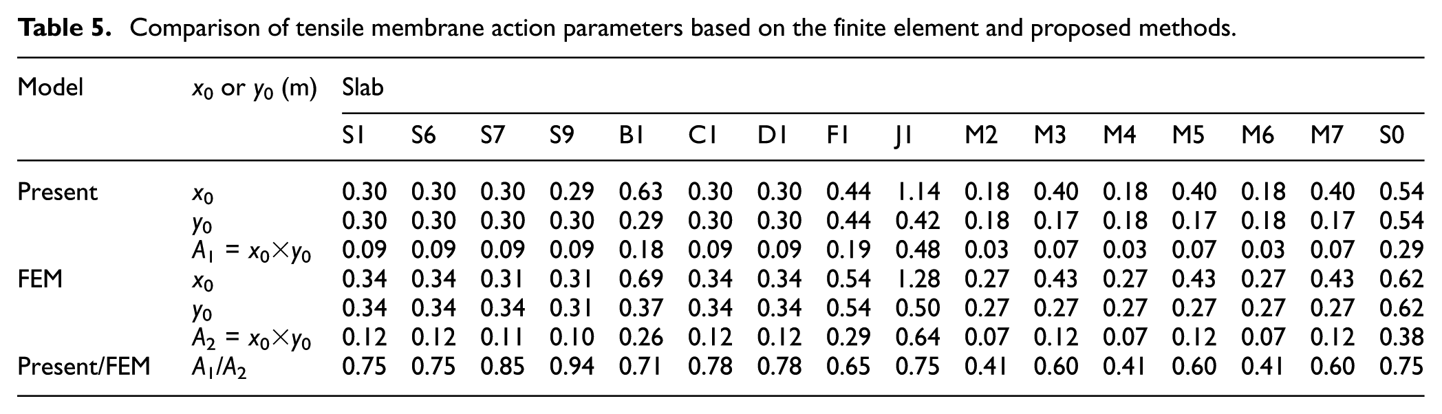
2. x₀ (or y₀) and the corresponding area (x₀×y₀) predicted by the proposed method and numerical model are shown in Table 5. The value of A₁/A₂ ranges from 0.41 to 0.94, with an average value of 0.67, indicating that the values of x₀ and y₀ for the concrete slabs obtained using the proposed method are smaller than those provided by the numerical model, especially for small-scale slabs. In all, this comparison indicates that the relationship given in equation (11) has a considerable effect on the key parameters of the proposed method.

Table 5.

Comparison of tensile membrane action parameters based on the finite element and proposed methods.

Model	x₀ or y₀ (m)	Slab
		S1	S6	S7	S9	B1	C1	D1	F1	J1	M2	M3	M4	M5	M6	M7	S0
Present	x ₀	0.30	0.30	0.30	0.29	0.63	0.30	0.30	0.44	1.14	0.18	0.40	0.18	0.40	0.18	0.40	0.54
	y ₀	0.30	0.30	0.30	0.30	0.29	0.30	0.30	0.44	0.42	0.18	0.17	0.18	0.17	0.18	0.17	0.54
	A₁ = x₀×y₀	0.09	0.09	0.09	0.09	0.18	0.09	0.09	0.19	0.48	0.03	0.07	0.03	0.07	0.03	0.07	0.29
FEM	x ₀	0.34	0.34	0.31	0.31	0.69	0.34	0.34	0.54	1.28	0.27	0.43	0.27	0.43	0.27	0.43	0.62
	y ₀	0.34	0.34	0.34	0.31	0.37	0.34	0.34	0.54	0.50	0.27	0.27	0.27	0.27	0.27	0.27	0.62
	A₂ = x₀×y₀	0.12	0.12	0.11	0.10	0.26	0.12	0.12	0.29	0.64	0.07	0.12	0.07	0.12	0.07	0.12	0.38
Present/FEM	A₁/A₂	0.75	0.75	0.85	0.94	0.71	0.78	0.78	0.65	0.75	0.41	0.60	0.41	0.60	0.41	0.60	0.75

Parameter analysis

Taking Slab C1 as an example, the effects of four parameters (θ_x,₀, θ_x,₁, $Δ {\bar{ε}}_{sx, 0}$ and $Δ {\bar{ε}}_{sx, 1}$ ) on the load–deflection curves are shown in Figure 8. As discussed above, the reference values of the four parameters are 0.05, 0.15, 1.0×10⁻⁵ and 8×10⁻⁴, respectively. For each case, one parameter was changed, and the other parameters were kept unchanged.

Figure 8.

Effects of four parameters (θ_x,₀, θ_x,₁, $Δ {\bar{ε}}_{sx, 0}$ and $Δ {\bar{ε}}_{sx, 1}$ ) on the slab’s load-carrying capacities as predicted by the proposed method.

As shown in Figure 8, four parameters have important effects on the load–deflection curves of the concrete slabs during the membrane action stage. On one hand, θ_x,₀ and $Δ {\bar{ε}}_{sx, 0}$ have considerable effects on entire load–deflection curves, and θ_x,₁ and $Δ {\bar{ε}}_{sx, 1}$ have important effects on the later load–deflection curves. On the other hand, the carrying capacities of the concrete slab decrease with increasing θ_x,₀ (or θ_x,₁), but they increase with increasing $Δ {\bar{ε}}_{sx, 0}$ (or $Δ {\bar{ε}}_{sx, 1}$ ). Clearly, this is due to the decrease or increase of the membrane action region (i.e. x₀ and y₀), as indicated in equations (2a) and (5b).

Conclusion

Based on the results of this study, the following conclusions can be drawn:

A new analytical method, based on five parts (four rigid plates and one centre region), the steel strain difference and two failure criteria, is established to predict the load-carrying capacity of concrete slabs during the tensile membrane stage. In addition, the linear steel strain difference–angle relationship is proposed in this article.

The method can reasonably predict the nonlinear load–deflection curves, tensile membrane region and failure modes of the concrete slabs. Meanwhile, the tensile membrane region predicted by the proposed method is relatively smaller than the numerical results.

The angle, steel strain difference and their relationship have considerable effects on the load–carrying capacity of the concrete slabs; the load-carrying capacity of one slab decreases with increasing angle and increases with increasing steel strain difference.

Footnotes

Appendix 1 Declaration of conflicting interests

The author(s) declared no potential conflicts of interest with respect to the research, authorship and/or publication of this article.

Funding

The authors disclosed receipt of the following financial support for the research, authorship, and/or publication of this article: This research was supported by the China Postdoctoral Science Foundation (grant no. 2014M560461 and 2016T90525) and National Natural Science Foundation of China (grant no. 51408594). The authors are grateful for this support.

References

(2017) Fire and post-fire carrying capacity study of two-way restrained concrete slabs. Master thesis, China University of Mining and Technology, Xuzhou, China (in Chinese).

Bailey

(2001) Membrane action of unrestrained lightly reinforced concrete slabs at large displacements. Engineering Structures 23(5): 470–483.

Bailey

Toh

(2007) Small-scale concrete slab tests at ambient and elevated temperatures. Engineering Structures 29(10): 2775–2791.

Bailey

Toh

(2010) Behavior of concrete floor slabs at ambient and elevated temperatures. Fire Safety Journal 42(6–7): 425–436.

Burgess

(2017) Yiled line plasticity and tensile membrane action in lightly-reinforced rectangular concrete slabs. Engineering Structures 138(1): 195–214.

Cameron

NJK

Usmani

(2005) New design method to determine the membrane capacity of laterally restrained composite floor slabs in fire. Part I: theory and method. The Structural Engineer 83(19): 28–33.

Dong

Fang

(2010) Determination of tensile membrane effects by segment equilibrium. Magazine of Concrete Research 62(1): 17–23.

GB50010-2010 (2011) Code for Design of Concrete Structures. Beijing, China: China Architecture & Building Press (in Chinese).

Ghoneim

McGregor

(1994) Tests of reinforced concrete plates under combined inplane and lateral loads. ACI Structural Journal 91(1): 19–30.

10.

Herraiz

(2016) Robustness of flat slab structures subjected to a sudden column failure scenario. PhD Thesis, ETH Zurich, Zurich.

11.

Herraiz

Vogel

(2016) Novel design approach for the analysis of laterally unrestrained reinforced concrete slabs considering membrane action. Engineering Structures 123(9): 313–329.

12.

Huang

Burgess

Plank

(2003a) Modeling membrane action of concrete slabs in composite buildings in fire. I: theoretical development. Journal of Structural Engineering 129(8): 1093–1102.

13.

Huang

Burgess

Plank

(2003b) Modeling membrane action of concrete slabs in composite buildings in fire. II: validations. Journal of Structural Engineering 129(8): 1103–1112.

14.

Kodur

VKR

Dwaikat

(2008) A numerical model for predicting the fire resistance of reinforced concrete beams. Cement Concrete Composite 30(5): 431–443.

15.

Guo

Zhou

(2007) Modeling of membrane action in floor slabs subjected to fire. Engineering Structures 29(6): 880–887.

16.

Omer

Izzuddin

Elghazouli

(2010) Failure of unrestrained lightly reinforced concrete slabs under fire – part I: analytical models. Engineering Structures 32(9): 2631–2646.

17.

Taylor

Maher

DRH

Hayes

(1966) Effect of the arrangement of reinforcement on the behaviour of reinforced concrete slabs. Magazine of Concrete Research 18(55): 85–94.

18.

Wang

Dong

Zhou

(2013) Nonlinear numerical modeling of two-way reinforced concrete slabs subjected to fire. Computers and Structures 119: 23–36.

19.

Wang

Dong

Yuan

et al . (2015) New failure criterion to determine the load carrying capacity of two-way reinforced concrete slabs. Advances in Structural Engineering 18(2): 221–236.

20.

(2005) Concrete Structures. 2th ed. Beijing, China: Tsinghua Press (in Chinese).

21.

Zhang

Dong

Fang

(2017) Modification of segment equilibrium method through considering tensile membrane effects and its application in two-way concrete slabs. Engineering Mechanics 34(3): 204–210 (240) (in Chinese).

New analytical method for determining the load-carrying capacity of two-way simply supported concrete slabs

Abstract

Keywords

Introduction

Proposed method

Assumptions

Initial angle

Analytical mode

Model parameters

Determination of θy

Determination of x0 and y0

Steel strain difference

Angle–steel strain difference relationship

Equilibrium equations

Internal force equilibrium equations

Equilibrium equations of different regions

Load capacity

Failure criteria

Compressive failure due to concrete crushing

Reinforcement failure

Verification and discussion

Comparison of the proposed method with experimental and other theoretical results

Comparison with numerical results

Parameter analysis

Conclusion

Footnotes

Appendix 1

Declaration of conflicting interests

Funding

References

Determination of θ_y

Determination of x₀ and y₀