Dynamic analysis of coupled train–track–bridge system subjected to debris flow impact

Abstract

With the increasing popularity of high-speed railway, more and more bridges are being constructed in Western China where debris flows are very common. A debris flow with moderate intensity may endanger a high-speed train traveling on a bridge, since its direct impact leads to adverse dynamic responses of the bridge and the track structure. In order to address this issue, a dynamic analysis model is established for studying vibrations of coupled train–track–bridge system subjected to debris flow impact, in which a model of debris flow impact load in time domain is proposed and applied on bridge piers as external excitation. In addition, a six-span simply supported box girder bridge is considered as a case study. The dynamic responses of the bridge and the running safety indices such as derailment factor, offload factor, and lateral wheel–rail force of the train are investigated. Some influencing factors are then discussed based on parametric studies. The results show that both bridge responses and running safety indices are greatly amplified due to debris flow impact loads as compared with that without debris flow impact. With respect to the debris flow impact load, the boulder collision has a more negative impact on the dynamic responses of the bridge and train than the dynamic slurry pressure. Both the debris flow impact intensity and train speed determine the running safety indices, and the debris flow occurrence time should be also carefully considered to investigate the worst scenario.

Keywords

debris flow dynamic analysis high-speed railway running safety train–track–bridge interaction

Introduction

Debris flows, which contain varying amounts of water, mud, sand, gravel, and boulders running over steep slopes and rushing through steam channels are a catastrophic geological hazard in mountain areas throughout the world (Cui et al., 2015; Hu et al., 2011). China is one of the countries where debris flows frequently occur. Statistics showed that approximately 45% area of China had suffered from debris flows (Hong et al., 2015; Liang et al., 2012). Debris flow hazards in China are mainly distributed in Yunnan, Xizang, Sichuan, Qinghai, Guizhou, and Gansu Provinces. For example, the most severe railway disaster in China occurred on 9 July 1981 in Sichuan province, in which two 15 m high piers of the Liziyida bridge on the Chengdu-Kunming Railway were destroyed by a debris flow, resulting in 400 casualties (Kang et al., 2004). Despite the hazardous consequences of debris flows, more high-speed railway lines (e.g. the Chengdu-Lanzhou Railway and the Sichuan-Tibet Railway) still need to be constructed in mountainous areas, due to the demand of economic development. According to Zhang and Zhang (2017), the recent strong earthquake events, that is, 2008 Wenchuan Earthquake and 2013 Ya’an Earthquake have caused significant geological changes and triggered many debris flows during rainstorms in recent years, and the debris flow disasters will be more frequent in the coming decades.

Debris flows cause damage mainly in three ways: deposition, erosion, and direct impact. The impact load of a debris flow often causes structural destruction and is a key element in bridge design and risk assessment (Deng et al., 2016). Although the probability of occurrence for an extreme debris flow is relatively small, a common debris flow with moderate intensity may cause serious consequences to the running of a high-speed train on a bridge. The main reason is that the debris flow impact load generates dislocation of bridge bearings, displacement and vibration of bridge girders, uneven deformation of the track, and so on; these adverse factors may threaten train running safety, and in the most severe case, the train may even derail from the track.

The train–bridge interaction is a classic topic of railway dynamics. There have been many investigations on the dynamic behavior of the train–bridge system, such as Yang et al. (2004), Xia et al. (2011), and Zhai and Xia (2011). With the increasing popularity of high-speed railway in China, various bridges have been systematically studied focusing on safety evaluation and design envelope of bridge dynamic characteristics; meanwhile, a mature methodology of train–track–bridge interaction has been developed. Some recent studies are aiming at improving the computational accuracy and/or efficiency (Li et al., 2013; Zhu et al., 2018), while others are focusing on the random vibration characteristics due to uncertainty of track irregularities (Zhu et al., 2016; Jin et al., 2017).

Besides the self-excitation vibrations of the train–bridge system, the external loads induced vibrations are attracting more and more attentions, such as wind (Wu et al., 2017; Zhang et al., 2015), earthquake (Jin et al., 2016; Xu and Zhai, 2017), and sea wave (Fang et al., 2017). The scenarios of train–bridge system subjected to collision loads, like vessel, vehicle, and floating ice, were also investigated by Xia et al. (2014, 2013). In these studies, one of the most challenging work is to quantify external loads. Obviously, dynamic analysis is much more complicated for a combined case in which one external load is applied when a train travels on a bridge. Safety issue due to debris flow impact is a major concern for a high-speed railway bridge in service. However up to now, relevant investigations have not yet been documented.

The study of the train running safety evaluation on a bridge subjected to debris flow impact load can be generalized into several aspects: the model of debris flow impact load, the train–track–bridge system model, the impact mechanism between debris flow and bridge, the dynamic response solution method, the dynamic safety indices, and the vibration mitigation measures (Zhang et al., 2018). In this article, it is the first time to investigate how the debris flow impact load affects the dynamic response of the train–track–bridge system and running safety of high-speed trains.

This article is organized as follows. A debris flow impact load model is first proposed based on the latest research findings, in which the time history of the debris flow impact load is assumed. The dynamic analysis model is then established for studying vibrations of coupled train–track–bridge system subjected to debris flow impact, where the debris flow impact load is regarded as the external excitation applied on bridge piers. Based on that, a multi-span simply supported box girder bridge on the Chengdu-Lanzhou Railway is selected as the case study, and the numerical simulation of a CRH2 high-speed train running on the bridge with applying debris flow impact load on bridge piers is carried out. The dynamic response of the bridge and the running safety indices of high-speed train are analyzed. Finally, parametric studies are carried out to investigate the influences of debris flow occurrence time, train operation speed, and debris flow impact intensity.

Model of debris flow impact load

Debris flow impact process

Debris flow is a kind of solid-fluid two-phase flow; the debris components and grain size distributions have a significant influence on its impact force (He et al., 2016). The fluid phase of the debris flow is composed of slurry (including small-sized coarse particles), which surges down as a continuous fluid. The solid phase is boulders, which moves as suspended load and/or bed load in the fluid phase. According to the observations in the laboratory and on the site (Bugnion et al., 2012; Cui et al., 2015; Hu et al., 2011; Scheidl et al., 2012), the debris flow impact process can be divided into three stages (see Figure 1(a)):

Stage 1: the rapid and powerful impact of the flow head. The impact time in this stage is usually about 0.8–1.0 s, from the time when the debris flow touches the pier till the time the flow depth reaches a maximum. Significant flow turbulence phenomenon can be observed if the debris flow density is lower than 2000 kg/m³. During this stage, the impact load increases rapidly, and the peak impact load usually appears earlier than the maximum flow depth. The boulders are easily to be transported due to the intense energy of the flow head. According to Zhang et al. (2007), the impact duration of a single boulder is about 0.01 s, which can be modeled as a triangular impulse. The boulders suspend in the middle height of a dilute debris flow or in the surface layer of a viscous one.

Stage 2: the continuous and steady impact of the flow body. In this stage, the flow turbulence becomes very weak, and the debris flow approximates a steady laminar flow. The flow depth in stage 2 is smaller than that in stage 1; whereas it is very hard to determine the difference between them. It is measured that the averaged continuous pressure of the flow body equals to 0.68 times of the peak pressure of the flow head (Cui et al., 2015). The occurrence of boulder impacts is random; however, it was observed that the majority of them took place in the front part of the flow body.

Stage 3: the slip flow of the flow tail. The velocity becomes much lower, and the impact pressure is much smaller than the rapid impact pressure. The destructive effect of the flow tail is generally limited.

Figure 1.

Debris flow: (a) typical impact process, (b) depth, and (c) impact load versus time.

General formulae

There are several models for the estimation of debris flow impact load. The models can be classified into hydrodynamic and solid collision models. The hydrodynamic model refers to the dynamic pressure provided by the slurry, and the solid collision model is associated with the boulder.

Dynamic pressure of slurry

The formula for dynamic pressure of slurry is derived from fluid momentum balance and Bernoulli equation, expressed as

P_{slurry} = α ρ_{s} v_{s}^{2}

(1)

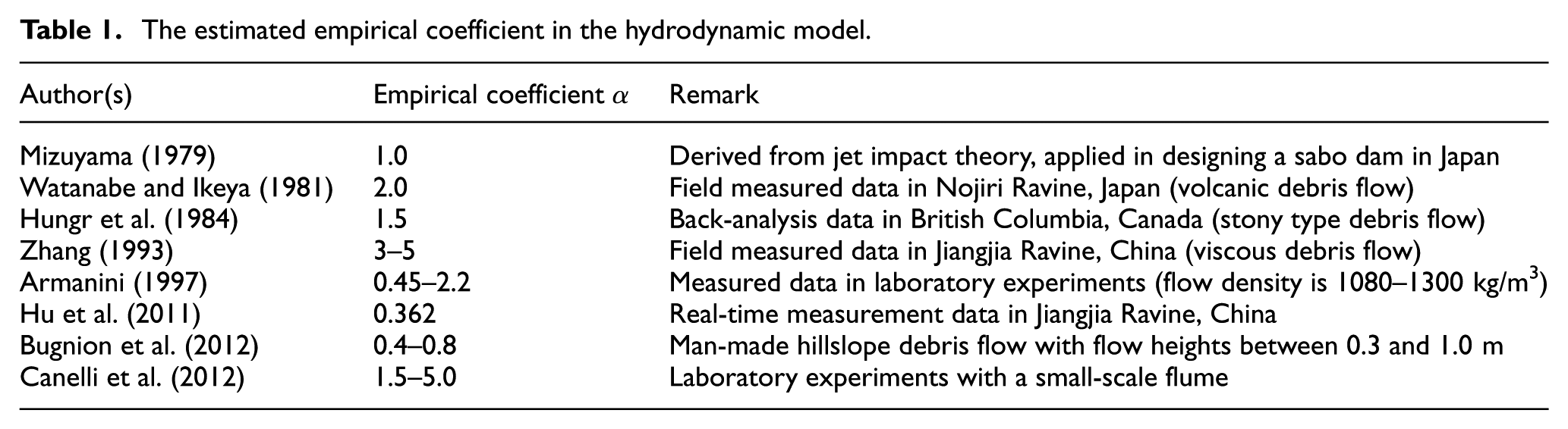
where P_slurry is the impact pressure of slurry; α is the empirical coefficient; ρ_s and v_s are the density and velocity of slurry, respectively. The empirical coefficient α depends on the flow type, that is, viscous, low-viscous, or transitional debris flow due to density, yield stress, and bed slope. The values of the empirical coefficient have been estimated based on laboratory experiments and field measurements, as shown in Table 1. It can be found that because of the variations in debris flow composition, the empirical coefficient α varies vastly. In addition, the impact pressure also depends on the geometric characteristics of the structure, for example, barrier, wall, or pier (Bugnion et al., 2012). As reported, the empirical coefficient could be a function of the dimensionless Froude number, which is the ratio between inertial and gravitational forces of the flow mass (Cui et al., 2015). However, a model for determining the empirical coefficient α is still lacking that can be applied to all types of flow or some sorts of debris flow.

Table 1.

The estimated empirical coefficient in the hydrodynamic model.

Author(s)	Empirical coefficient α	Remark
Mizuyama (1979)	1.0	Derived from jet impact theory, applied in designing a sabo dam in Japan
Watanabe and Ikeya (1981)	2.0	Field measured data in Nojiri Ravine, Japan (volcanic debris flow)
Hungr et al. (1984)	1.5	Back-analysis data in British Columbia, Canada (stony type debris flow)
Zhang (1993)	3–5	Field measured data in Jiangjia Ravine, China (viscous debris flow)
Armanini (1997)	0.45–2.2	Measured data in laboratory experiments (flow density is 1080–1300 kg/m³)
Hu et al. (2011)	0.362	Real-time measurement data in Jiangjia Ravine, China
Bugnion et al. (2012)	0.4–0.8	Man-made hillslope debris flow with flow heights between 0.3 and 1.0 m
Canelli et al. (2012)	1.5–5.0	Laboratory experiments with a small-scale flume

Impact force of boulder

The measurements by Zhang (1993) showed that the single boulder collision against structures led to significant impact forces. At present, the so-called solid collision model based on the Hertz law is preferred (Huang et al., 2007). However, the Hertz elastic contact theory overestimates the boulder impact force, and thus, some scholars suggested alternative models that consider elastic–plastic property of materials on the mechanical contact characteristics (Chen et al., 2017; He et al., 2016). Considering these factors, the following formulae can be used to estimate the impact force exerted by boulders (Chen et al., 2017)

F_{boulder} = k_{c 1} k_{c 2} k_{c 3} [\frac{4}{3 π {(k_{1} + k_{2})}^{0.4}}] {(\frac{5 ρ_{b} π^{2}}{4})}^{0.6} V_{b}^{0.8} R_{b}^{2}

(2)

k_{1} = \frac{1 - μ_{1}^{2}}{π E_{1}}, k_{2} = \frac{1 - μ_{2}^{2}}{π E_{2}}

(3)

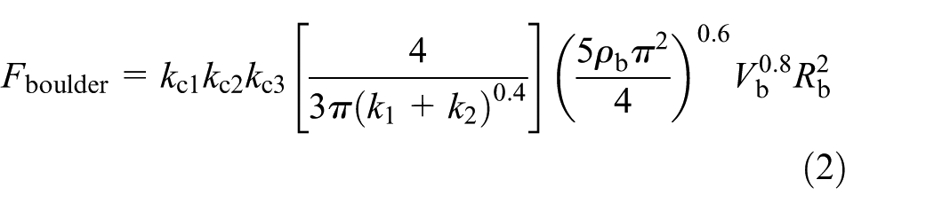
where F_boulder is the boulder impact force; ρ_b, V_b, and R_b are the density, velocity, and diameter of boulder, respectively; μ₁ and μ₂ are the Poisson’s ration of boulder and pier, respectively; E₁ and E₂ are the Young’s moduli of boulder and pier, respectively; k_c1, k_c2, and k_c3 are three correction factors, which are associated with the influences of elastic–plastic property of pier material, relative size between boulder and pier, and pier displacement during the impact process. Equation (2) gives reasonable estimation of the boulder impact force and matches well with field observations.

Proposed time history of a debris flow impact load

The acquisition of debris flow impact loads under real-world conditions is a great challenge. In order to carry out simulations in this study, a typical debris flow impact load has to be assumed. Considering the debris flow impact process, the time history of debris flow impact load is proposed in this article, as shown in Figure 1(b) and (c). The details are described as follows.

Three stages of the debris flow are presented as shown in Figure 1(a). The starting and ending times of the three stages are 0–t₁, t₁–t₂, and t₂–t₃, respectively. t₁ is usually about 0.8–1.0 s, while t₂ depends on the scale of the debris flow. Boulder collisions take place in the flow head and the front part of flow body.

H _L and H_H are the depths of flow body and head, respectively, which can be determined from the geologic data at the bridge site. The depth variation of flow head is neglected for simplicity. The heights of boulders are 0.5H_L and H_L for dilute and viscous debris flow, respectively.

Equation (2) is used to calculate the slurry impact pressure of flow body p_L. The peak pressure of flow head p_H equals to p_L / 0.68. In the flow head, the slurry impact pressure gradually increases and reaches the maximum at the time of 0.5t₁.

The boulder impact force is computed based on Equation (3). The single boulder impact is represented by a triangular impulse with a duration of 0.01 s. Multiple boulder impacts may occur, and thus this article considers a group of boulders (e.g. 10) continuously striking the pier. The first round of boulder impact occurs at 0.5t₁, and the second one takes place along with the flow body (e.g. at the time of t₁ + 1).

It should be noted that although the proposed time history of the debris flow impact load may be different from real scenario, the main features of debris flow impact load have been taken into account. In addition, parametric studies are conducted in the following sections to discuss the influences of impact intensity and occurrence time of debris flow impact load.

Model of coupled train–track–bridge system subjected to debris flow impact

The established analysis model of coupled train–track–bridge system subjected to debris flow impact is a three-dimensional dynamic system composed of three subsystems, that is, the train subsystem, the track subsystem, and the bridge subsystem. Three subsystems are coupled by wheel–track interaction and track–bridge interaction. The debris flow impact load is regarded as an external excitation acting on several piers of the bridge, as shown in Figure 2.

Figure 2.

Dynamic analysis model.

Coupled train–track–bridge system

Train subsystem

The train subsystem is composed of several independent vehicles (i.e. motor cars and trailer cars for a modern high-speed train). Each vehicle consists of seven rigid bodies: a car body, two bogies, and four wheelsets, which are connected by spring-damping connections representing the primary and secondary suspensions. Each rigid body has five degrees-of-freedoms (DOFs) in the Y, Z, RX, RY, and RZ directions, that is, lateral, vertical, rolling, yawing, and pitching movements. Therefore, the idealized model for each vehicle has 35 DOFs. The motion equation of the train subsystem can be derived according to the D’Alembert’s principle, expressed in the matrix form as

M_{v} {\overset{\cdot\cdot}{u}}_{v} + C_{v} {\overset{\cdot}{u}}_{v} + K_{v} u_{v} = R_{v}

(4)

where M _v, C _v, and K _v are the mass, damping, and stiffness matrices of the train, respectively; u _v, ${\overset{\cdot}{u}}_{v}$ , and ${\overset{\cdot\cdot}{u}}_{v}$ are the generalized displacement, velocity, and acceleration vectors of the train; and R _v is the generalized force vector of the train.

Track subsystem

The track submodel shown in Figure 2 represents the double-block ballastless track, which is used in the case study. For the double-block ballastless track, the sleeper blocks are directly precast into the track slab and there is no elasticity between the track slab and the concrete base on the bridge deck; therefore, the left and right rails are treated as Euler beams which are supported at discrete points by spring-damping elements, representing the elasticity and damping of rail fastenings. The rails vibrate in three directions, that is, vertical, lateral, and torsional movements. The motion equation of the track subsystem is written as

M_{t} {\overset{\cdot\cdot}{u}}_{t} + C_{t} {\overset{\cdot}{u}}_{t} + K_{t} u_{t} = R_{t}

(5)

where M _t, C _t, and K _t are the mass, damping, and stiffness matrices of the track, respectively; u _t, ${\overset{\cdot}{u}}_{t}$ , and ${\overset{\cdot\cdot}{u}}_{t}$ are the generalized displacement, velocity, and acceleration vectors of the track; and R _t is the generalized force vector of the track.

Bridge subsystem

Bridge structures can be modeled by the finite element method with different element types, such as spatial beam element, spatial bar element, plate/solid element, and other special elements. For a multi-span simply supported box girder bridge, the spatial beam element is usually adopted to model the beam and the pier, which can achieve satisfying precision. The connection between beam and pier is simulated by master-slave nodes according to the actual constraint condition at each bearing location. In order to consider the effects of the foundation stiffness, the equivalent-stiffness model is used by exerting six equivalent spring stiffness at the bottom of cushion caps. The dynamic equation of the bridge subsystem is

M_{b} {\overset{\cdot\cdot}{u}}_{b} + C_{b} {\overset{\cdot}{u}}_{b} + K_{b} u_{b} = R_{b}

(6)

where M _b, C _b, and K _b are the mass, damping, and stiffness matrices of the bridge, respectively; u _b, ${\overset{\cdot}{u}}_{b}$ , and ${\overset{\cdot\cdot}{u}}_{b}$ are the generalized displacement, velocity, and acceleration vectors of the bridge; and R _b is the generalized force vector of the bridge.

More details of the motion equations (4) and (5) can be found in Zhai and Xia (2011). The two equations are coupled with the wheel–rail interaction model, in which the nonlinear Hertzian elastic contact theory is used to calculate the wheel–rail normal contact forces, and the Kalker’s linear creep theory is considered to calculate the tangential wheel–rail creep forces. Equations (5) and (6) are coupled with the track–bridge interaction model, in which a series of point-to-point spring-damping connections at each contact point between the rail and the bridge deck is defined. Therefore, once the vibrations of the rail and bridge are obtained, the interaction forces between them can be determined.

Debris flow impact load

In order to calculate the dynamic response due to the train–track–bridge interaction combined with a debris flow impact load, the time history of the debris flow impact load is required, which has been assumed in the previous section. The time histories of debris flow impact load are taken as external load input to the bridge subsystem model. Thus, the dynamic equation of the bridge subsystem can be rewritten as

M_{b} {\overset{\cdot\cdot}{u}}_{b} + C_{b} {\overset{\cdot}{u}}_{b} + K_{b} u_{b} = R_{b} + R_{d}

(7)

where R _d is associated with the debris flow impact load acting on the bridge.

Solution strategy

Equations (4), (5), and (7) comprise a large-scale nonlinear dynamic system, which involves vehicle suspension, wheel–rail contact and creep, as well as other nonlinear factors. In the numerical analysis, a fast explicit–implicit integration method is used to solve the vehicle and track subsystems, and the Newmark-β integration is used to solve the dynamic response of the bridge subsystem. This hybrid explicit–implicit integration method has a high efficiency and has been proved by Zhai and Xia (2011). A Fortran program is compiled based on the formulation derived above and is used to perform the following case study.

Case study

Bridge description

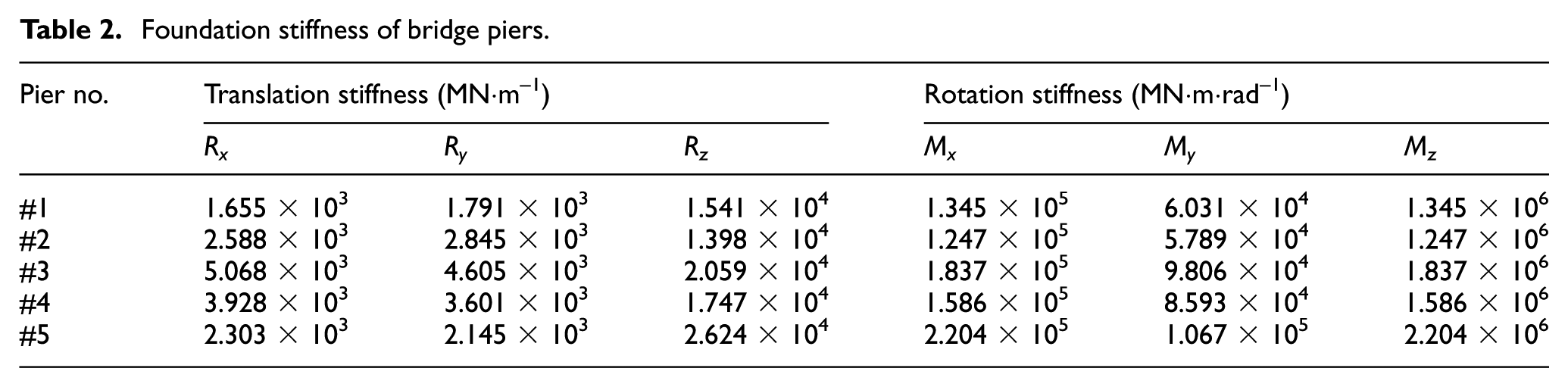
The case study investigates a multi-span simply supported box girder bridge situated on the Chengdu-Lanzhou Railway in Western China, where the debris flow disaster is very common. Figure 3 gives the general layout of the bridge, as well as the main dimensions of the beam and pier cross sections. The main beams are box girders, with the same cross section dimensions for two different spans (i.e. 24 and 32 m beams). A single track, namely the double-block ballastless track is laid on the bridge deck. All the piers are of round-ended cross sections, and the group-pile foundation is used. The support stiffnesses of the foundations are calculated by using the “m” method, as listed in Table 2.

Figure 3.

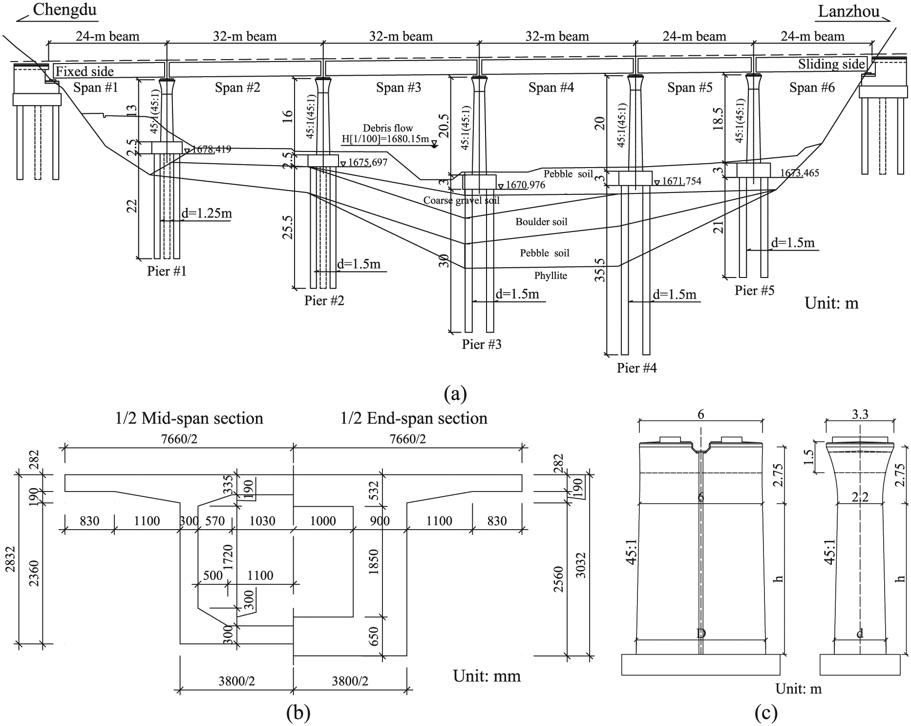
The Walnut Ravine Bridge on the Chengdu-Lanzhou Railway: (a) general layout; main dimensions of (b) the beam and (c) pier cross sections.

Table 2.

Foundation stiffness of bridge piers.

Pier no.	Translation stiffness (MN·m^–1)			Rotation stiffness (MN·m·rad^–1)
	R_x	R_y	R_z	M_x	M_y	M_z
#1	1.655 × 10³	1.791 × 10³	1.541 × 10⁴	1.345 × 10⁵	6.031 × 10⁴	1.345 × 10⁶
#2	2.588 × 10³	2.845 × 10³	1.398 × 10⁴	1.247 × 10⁵	5.789 × 10⁴	1.247 × 10⁶
#3	5.068 × 10³	4.605 × 10³	2.059 × 10⁴	1.837 × 10⁵	9.806 × 10⁴	1.837 × 10⁶
#4	3.928 × 10³	3.601 × 10³	1.747 × 10⁴	1.586 × 10⁵	8.593 × 10⁴	1.586 × 10⁶
#5	2.303 × 10³	2.145 × 10³	2.624 × 10⁴	2.204 × 10⁵	1.067 × 10⁵	2.204 × 10⁶

In the subsequent sections, two types of dynamic analyses are carried out. The first simulation focuses on the dynamic responses solely induced by a debris flow impact. The second one is to calculate dynamic responses due to the train–track–bridge interaction combined with debris flow impact load.

Vibrations of the bridge solely induced by debris flow impact

Calculation model

A detailed three-dimensional finite element model of the track and bridge is built by ANSYS software, as shown in Figure 4. In order to consider the track details, the box girder slabs (i.e. top slab, bottom slab, web, and flange) are modeled with plate elements. The rails, piers, and cushion caps are regarded as beam elements. For the connections between each components, several spring-damping elements are added to simulate the isolating effect of the rail fastenings. One layer of plate elements is used to model the ballastless track. A rigid connection condition is assumed between the ballastless track and the bridge deck, which is consistent with the bridge construction technique in practice. The stiffness and damping of the rail fastenings are 50 MN/m and 70 kN•s/m in the vertical direction, respectively. In the lateral direction, the corresponding values are 42 MN/m and 35 kN•s/m, respectively. The distance between adjacent fastenings is 0.6 m. The length of the rails out of each side of the bridge is 90 m, and they are assumed to be laid on the ground using spring-damping elements. The ends of the rails are assumed to be fixed. The pile foundation stiffness is considered by using six equivalent spring stiffnesses at the bottom of cushion caps. This model contains 17,426 elements with the maximum element size of 0.5 m. In the loading area, the elements are of smaller size.

Figure 4.

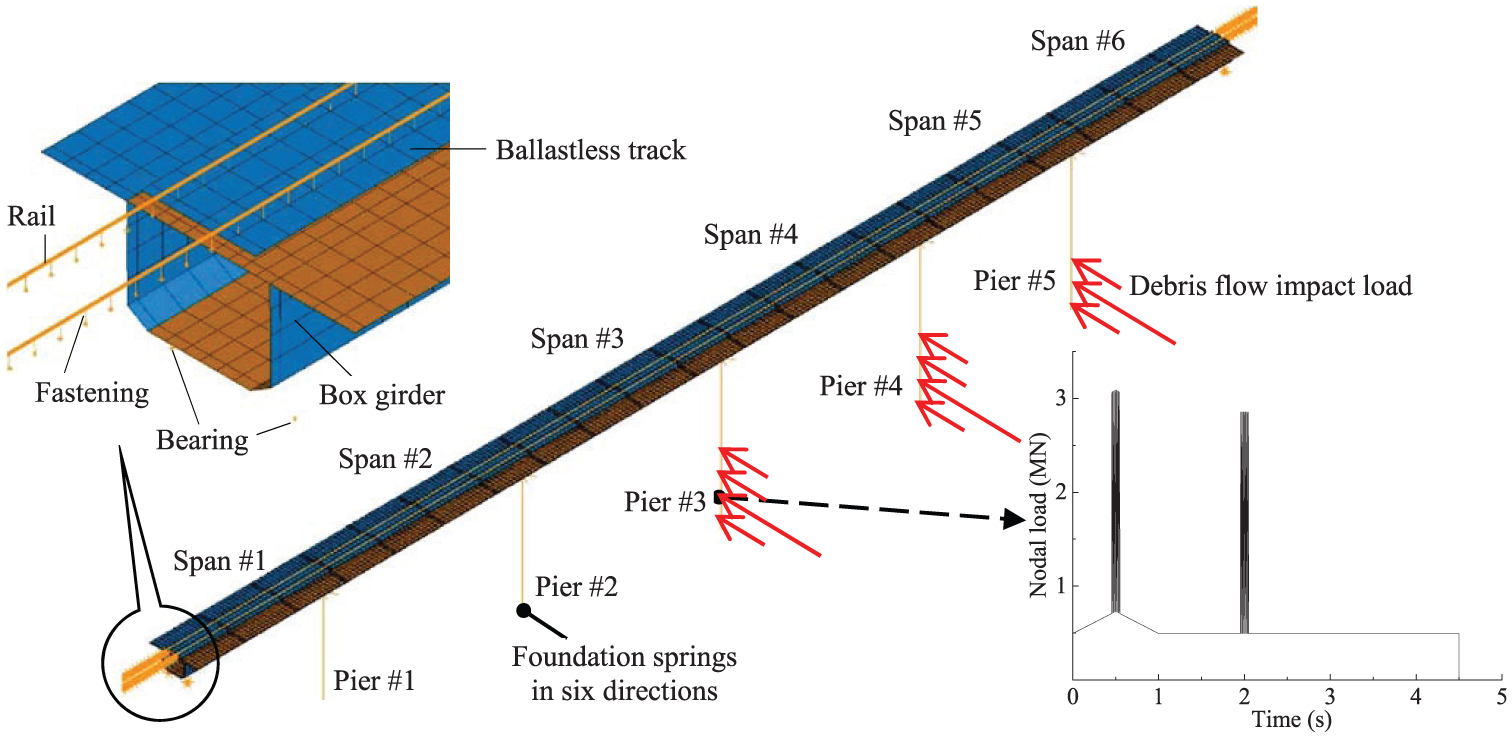
Three-dimensional finite element model of the track and bridge.

As shown in Figure 4, debris flow impact loads are applied on piers by using concentrated nodal forces in the horizontal direction. The details of the debris flow load are described as follows.

According to the geological data, three piers labeled #3, #4, and #5 are located in the debris flow ravine with a 100-year-return-period elevation of 1680.15 m (also shown in Figure 3(a)). Thus, the heights of the debris flow corresponding to Piers #3, #4, and #5 are 6.174, 5.396, and 3.685 m, respectively.

The velocity of the 100-year-return-period debris flow slurry is estimated as 4.23 m/s, with a density of 1800 kg/m³. Therefore, the dynamic pressures of debris flow head and body are 189 and 128 kPa, respectively, based on an empirical coefficient of 4.0 (see equation (1)).

The diameter and density of boulders are 1 m and 2650 kg/m³, respectively. A group of 10 boulders is considered to continuously impact Piers #3, #4, and #5 at a half height of the debris flow slurry. The first round of collision occurs at 0.5 s, and the second round takes place at 2 s. The total duration of each round of impact is 0.1 s. The calculated impact forces of the boulders acting on Piers #3, #4, and #5 are 2152, 2284, and 2395 kN based on equation (2), respectively.

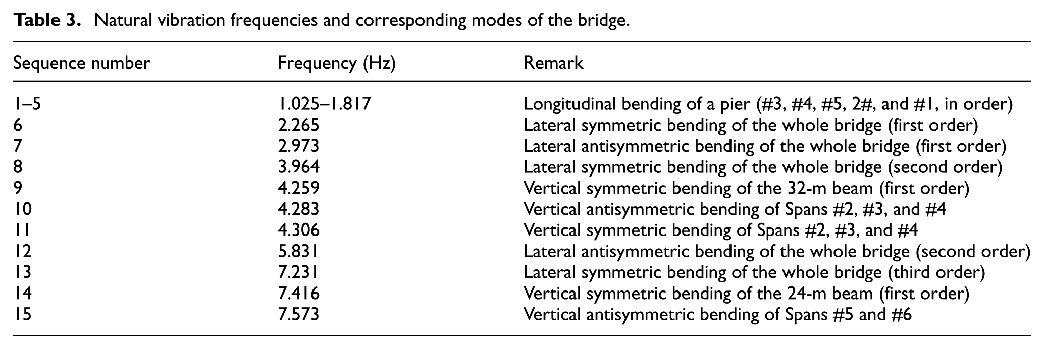
Natural vibration characteristics

The natural vibration characteristics including frequencies and mode shapes of the bridge are obtained, as listed in Table 3. The first five modes are the longitudinal bending of a certain pier (from the highest one to the lowest one) along with the longitudinal motion of the neighboring main beam. The first-order lateral symmetric bending of the whole bridge occurs at 2.265 Hz, which is lower than the first-order vertical symmetric bending frequencies of the 32 and 24 m beams (i.e. 4.259 and 7.416 Hz, respectively). Because the lateral stiffness of the box girder is very large, the lateral bending modes of the 32 and 24 m beams do not appear in the first 15 modes. However, the occurrences of lateral bending modes of the whole bridge, mainly characterized by the lateral vibration of piers, are very common in the first 15 modes (with sequence numbers 6, 7, 8, 12, and 13).

Table 3.

Natural vibration frequencies and corresponding modes of the bridge.

Sequence number	Frequency (Hz)	Remark
1–5	1.025–1.817	Longitudinal bending of a pier (#3, #4, #5, 2#, and #1, in order)
6	2.265	Lateral symmetric bending of the whole bridge (first order)
7	2.973	Lateral antisymmetric bending of the whole bridge (first order)
8	3.964	Lateral symmetric bending of the whole bridge (second order)
9	4.259	Vertical symmetric bending of the 32-m beam (first order)
10	4.283	Vertical antisymmetric bending of Spans #2, #3, and #4
11	4.306	Vertical symmetric bending of Spans #2, #3, and #4
12	5.831	Lateral antisymmetric bending of the whole bridge (second order)
13	7.231	Lateral symmetric bending of the whole bridge (third order)
14	7.416	Vertical symmetric bending of the 24-m beam (first order)
15	7.573	Vertical antisymmetric bending of Spans #5 and #6

Bridge and track responses

In Figure 5(a) and (b), the lateral displacements at the mid-span of Span #4 are shown in both time and frequency domains, respectively. In the case without train operation, it can be found that the displacement is significant under the debris flow impact loads. The maximum displacements under two rounds of boulders impact (i.e. at 0.5 and 2 s) are 4.16 and 3.99 mm, respectively. The dominant frequency component concentrates at 2.598 Hz, which is close to the first lateral bending frequency of the whole bridge, that is, 2.265 Hz. The bridge responses can be mapped to the rail on the bridge deck and lead to track irregularities, as shown in Figure 5(c). It is noted that the lateral displacement of the rail is significant in the range of Spans #3, #4, #5, and #6, as the debris flow impact loads are applied on Piers #3, #4, and #5. Out of this range, the lateral displacement of the rail quickly attenuates to zero. The maximum displacement of the rail is smaller than that of the box girder due to the elasticity of the track. However, the lateral rail displacement also experiences the peaks around the time of boulders impact.

Figure 5.

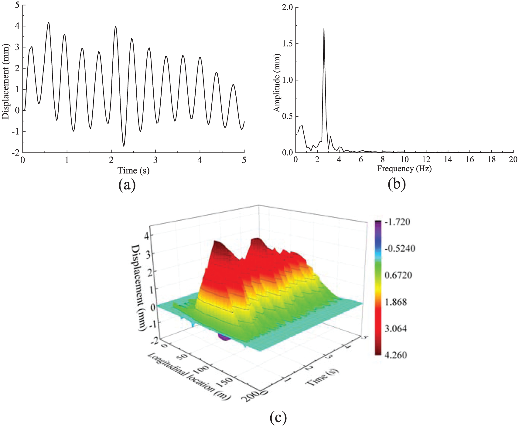
Lateral displacements solely induced by a debris flow impact without train operation: (a) time history, mid-span of Span #4; (b) spectrum, mid-span of Span #4; and (c) time history, rail.

Responses of coupled train–track–bridge system subjected to debris flow impact

Calculation condition

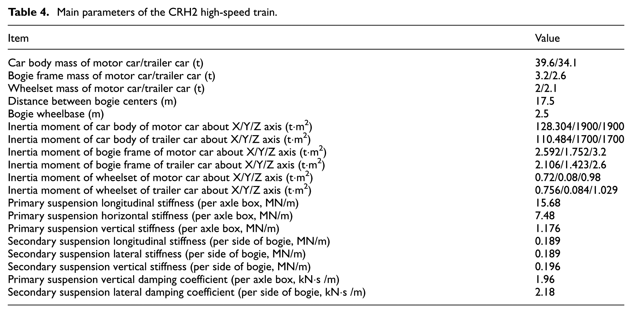
The CRH2 high-speed train is adopted for the dynamic analysis. It is composed of 2 × (M + T + M + M) cars, with M representing the motor car and T representing the trailer one, respectively. The main parameters are listed in Table 4. The measured track irregularity data on the Qinhuangdao-Shenyang High-Speed Railway are taken into consideration in this article, as plotted in Figure 6(a) and (b), representing the lateral and vertical irregularities, respectively. The train runs at a constant speed of 200 km/h in the simulations. The debris flow impact loads are applied at the time when the first wheelset of the first car arrives at the mid-span of Span #4, which ensures that all the eight cars of the train can pass Span #4 during the acting period of the debris flow load, in order to get the maximum train responses.

Table 4.

Main parameters of the CRH2 high-speed train.

Item	Value
Car body mass of motor car/trailer car (t)	39.6/34.1
Bogie frame mass of motor car/trailer car (t)	3.2/2.6
Wheelset mass of motor car/trailer car (t)	2/2.1
Distance between bogie centers (m)	17.5
Bogie wheelbase (m)	2.5
Inertia moment of car body of motor car about X/Y/Z axis (t·m²)	128.304/1900/1900
Inertia moment of car body of trailer car about X/Y/Z axis (t·m²)	110.484/1700/1700
Inertia moment of bogie frame of motor car about X/Y/Z axis (t·m²)	2.592/1.752/3.2
Inertia moment of bogie frame of trailer car about X/Y/Z axis (t·m²)	2.106/1.423/2.6
Inertia moment of wheelset of motor car about X/Y/Z axis (t·m²)	0.72/0.08/0.98
Inertia moment of wheelset of trailer car about X/Y/Z axis (t·m²)	0.756/0.084/1.029
Primary suspension longitudinal stiffness (per axle box, MN/m)	15.68
Primary suspension horizontal stiffness (per axle box, MN/m)	7.48
Primary suspension vertical stiffness (per axle box, MN/m)	1.176
Secondary suspension longitudinal stiffness (per side of bogie, MN/m)	0.189
Secondary suspension lateral stiffness (per side of bogie, MN/m)	0.189
Secondary suspension vertical stiffness (per side of bogie, MN/m)	0.196
Primary suspension vertical damping coefficient (per axle box, kN·s /m)	1.96
Secondary suspension lateral damping coefficient (per side of bogie, kN·s /m)	2.18

Figure 6.

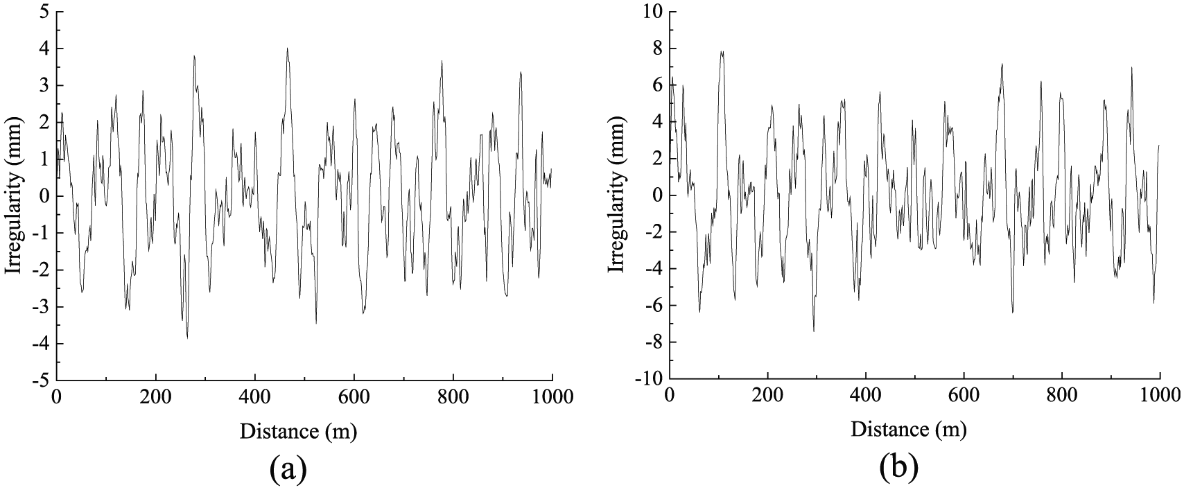
Measured track irregularities: (a) lateral and (b) vertical.

Bridge responses

The lateral displacement and acceleration histories at the mid-span of Span #4 are shown in Figure 7(a) and (c), respectively. These curves start to record responses at a distance of 10 m before the train enters into the bridge. In the case without debris flow impact, the bridge responses are caused by the running train; therefore, the time history curves are rather steady with very small values. While under the impact loads of debris flow, the bridge displacement and acceleration are significantly amplified, showing clear impact characteristics. The maximum displacement and acceleration are 3.60 mm and 1.55 m/s², respectively. Compared with Figure 5(a), the maximum lateral displacement at mid-span of Span #4 is slightly smaller, indicating that the train has an advantageous effect in reducing the debris flow impact induced responses. The maximum acceleration occurs during the boulders impact, which attributes to the short pulse effect.

Figure 7.

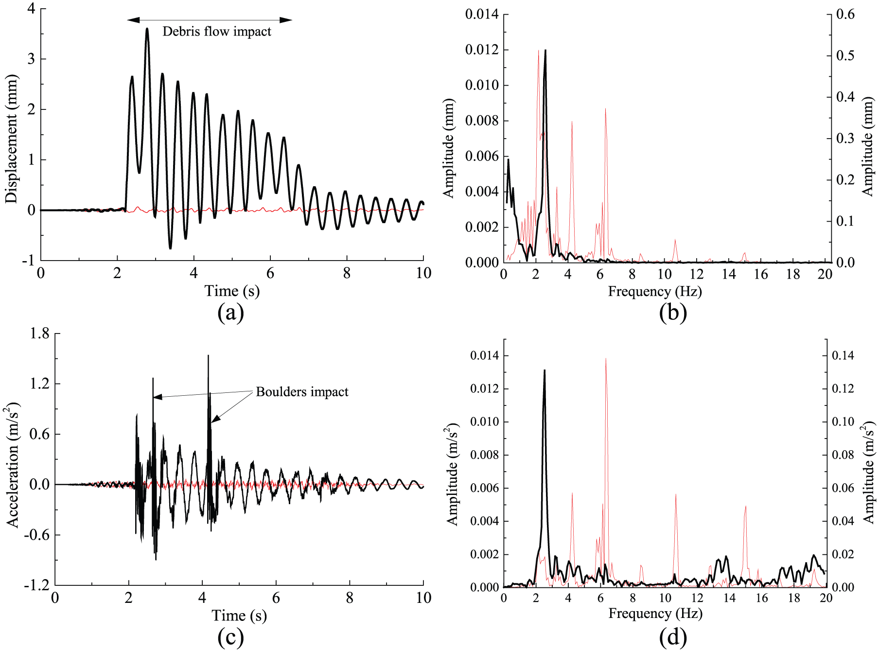
Lateral mid-span (Span #4) responses with debris flow impact (thick line) and without debris flow impact (thin line) at train speed 200 km/h: (a) time history, displacement; (b) spectrum, displacement; (c) time history, acceleration; and (d) spectrum, acceleration.

The frequency spectra of the bridge responses (lateral displacement and acceleration) are shown in Figure 7(b) and (d). In the case without debris flow impact, several peaks can be found and these frequency components are close to the lateral bending frequencies of the whole bridge although the train weight has some effects on the natural vibration characteristics of the bridge. For example, the peaks at 2.171 and 2.549 Hz are corresponding to the first-order lateral symmetric and antisymmetric bending frequency of the whole bridge (i.e. 2.265 and 2.973 Hz), respectively; the peak at 4.249 Hz is close to the second-order lateral symmetric bending frequency of the whole bridge (i.e. 3.964 Hz); the peak at 6.326 Hz is related to the second-order lateral antisymmetric bending frequency of the whole bridge (i.e. 5.831 Hz). In the case with debris flow impact, a peak appears at 2.549 Hz, which is similar to Figure 5(b); therefore, the forced vibration induced by debris flow impact loads rather than train loads plays a decisive role. A quasi-static component in the displacement spectrum can be found and the displacement response dominates in the low frequency range below 4 Hz. Different to the displacement spectrum, there is no quasi-static component in the acceleration spectrum and more high frequency contents are included.

Train responses

The evaluation indices for the running safety of a high-speed train include the derailment factor, the offload factor, and the lateral wheel–rail force (Zhai and Xia, 2011). Their definitions and the corresponding allowances are given below

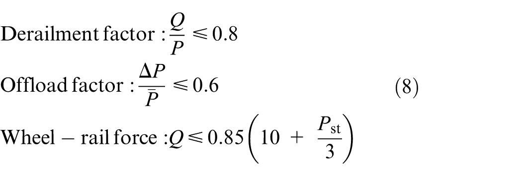
\begin{matrix} Derailment factor : \frac{Q}{P} \leq 0.8 \\ Offload factor : \frac{Δ P}{\bar{P}} \leq 0.6 \\ Wheel - rail force : Q \leq 0.85 (10 + \frac{P_{st}}{3}) \end{matrix}

(8)

where Q and P are the lateral and vertical wheel–rail forces, respectively; $Δ P$ is the offload vertical wheel–rail force; $\bar{P}$ is the average vertical wheel–rail force of the two wheels on a wheelset; P_st denotes the static wheelset load. The allowable lateral wheel–rail forces for the CRH2 motor car and trailer car are 46.0 and 41.8 kN, respectively.

Figures 8(a) to (c) show the time history curves of the derailment factor, the offload factor, and the lateral wheel–rail force of the second car with and without debris flow impact when the train runs on the bridge at 200 km/h. The second car is on Span #3 and about 10 m away from Pier #3 when the debris flow impact loads act on Piers #3, #4, and #5. It can be seen from the figures that the running safety indices of the train are strongly affected by the debris flow impact loads when the second car arrives at Span #4 during the first round of boulders impact. Although the dynamic slurry pressure has some influences on the train responses at the starting point of the debris flow impact (around 2 s), the running safety indices vary slightly. During the first round of boulders impact, the train responses are much influenced, indicating that the boulders impact is more intense and a short pulse load has more adverse effects on the running safety of the train. Under the debris flow impact loads, the maximum values of the running safety indices are greatly amplified: the derailment factor increases from 0.09 to 0.23, the offload factor increases from 0.11 to 0.23, and the lateral wheel–rail force increases from 6.0 to 16 kN. However, these indices are all within the corresponding safety allowances as the impact intensity is relatively small. In the second round of boulders impact, the second car is far away from Span #4, and thus the variation of train responses is not significant.

Figure 8.

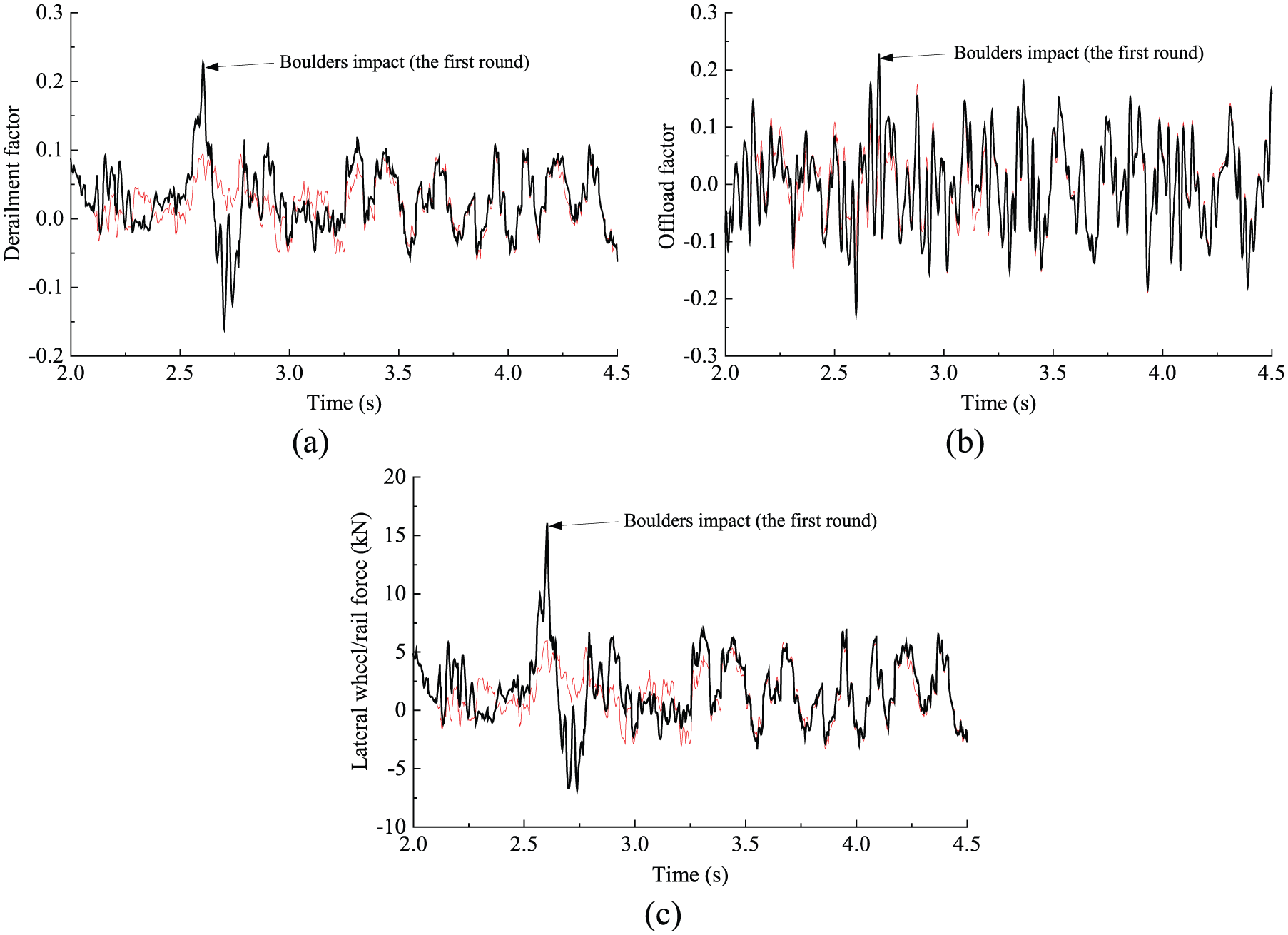
Train responses with debris flow impact (thick line) and without debris flow impact (thin line) at train speed 200 km/h: (a) derailment factor, (b) offload factor, and (c) lateral wheel–rail force.

Discussion

Influence of train location during debris flow impact

Train location on the bridge influences its responses when a debris flow impact load is applied. In order to find the most adverse location, the variation of train responses are calculated for different train locations. It is described in Figure 9(a), the location of the first wheelset is defined as the variate X, representing the distance from the first wheelset to Pier #3 (the first pier subjected to the debris flow impact). While keeping the parameters of the bridge, the train and the debris flow impact load unchanged, the train location X varies from −42 to 42 m with an increment of 6 m when the debris flow impact takes place. The total length of a vehicle is 26 m, and the distance between bogie centers and bogie wheelbase are 17.5 and 2.5 m, respectively.

Figure 9.

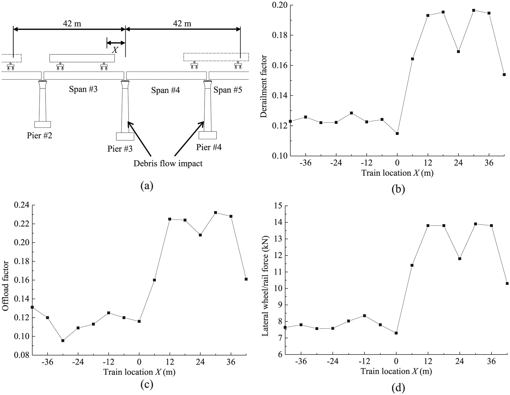
Distribution of train running safety indices versus train locations at train speed 200 km/h: (a) schematic plot of train locations, (b) derailment factor, (c) offload factor, and (d) lateral wheel–rail force.

The maximal derailment factors, offload factors, and lateral wheel–rail forces versus train locations are shown in Figures 9(b) to (d). It can be found that the train responses are larger when the train travels on Span #4 rather than on Span #3. The main reason is that the bridge vibration of Span #4 is larger than that of Span #3 due to the fact that the debris flow impacts acting on Piers #3, #4, and #5 simultaneously. Moreover, two peaks of train responses can be observed: the first one corresponds to the front bogie center situated at the mid-span of Span #4, and for the second one, the back bogie center arrives at the mid-span of Span #4.

Influence of train speed and debris flow impact intensity

With the same bridge and track irregularity parameters, the running safety of train is investigated by considering different train speeds and debris flow impact intensities. For all the simulations, the debris flow impact occurs when the second car is on Span #3 and about 10 m away from Pier #3. The maximum values of the running safety indices, which are taken from the corresponding time histories of the second car, are used for comparisons.

Figures 10 and 11 show the distribution of maximal derailment factors, offload factors, and lateral wheel–rail forces when the trains run on the bridge with the speeds of 160, 200, 240, 280, and 320 km/h, respectively. As the debris flow impact load consists of two parts—the dynamic slurry pressure and boulders impact—in the calculations, one part of them varies by using a multiplier while the other one remains unchanged. The horizontal dashed lines represent the allowance values given in equation (9). Referring to these figures, the influence of train speed and debris flow impact intensity on the running safety indices can be summarized as follows:

The greater the debris flow impact intensity and the higher the train speed, the higher the running safety indices including the derailment factor, the offload factor, and the lateral wheel–rail force.

For five train speeds (i.e. 160, 200, 240, 280, and 320 km/h), the increase tendency of running safety indices with the increasing debris flow impact intensity is obvious, especially when the train speed is greater than 280 km/h. At speeds lower than 240 km/h, the running safety indices increase moderately, indicating that a low operation speed is preferred when debris flows could happen in rainy seasons.

For the same multiplier, the increase rates of running safety indices in the case of changing boulders load intensity are larger than those in the case of changing slurry load intensity, namely boulders load causes more threats to the train operation than the slurry load. Therefore, boulders impact should be avoided in engineering practice.

The running safety of the train can be evaluated by the threshold curves between train speed and debris flow impact intensity, and thus an early warning system can be established according to the simulations of train–track–bridge system subjected to debris flow impact load.

Figure 10.

Distribution of train running safety indices versus slurry load intensity under different train speeds: (a) derailment factor, (b) offload factor, and (c) lateral wheel–rail force.

Figure 11.

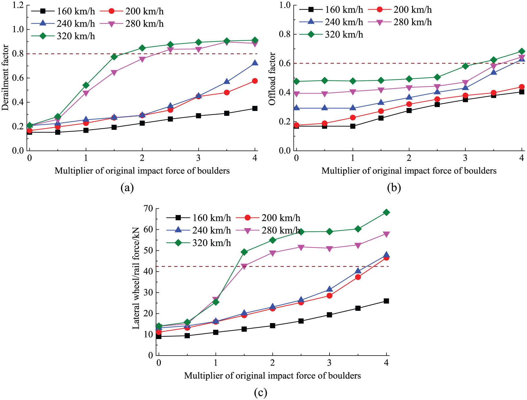
Distribution of train running safety indices versus boulders load intensity under different train speeds: (a) derailment factor, (b) offload factor, and (c) lateral wheel–rail force.

Conclusion

This article presents dynamic analysis model of a train–track–bridge system subjected to debris flow impact load. Through a case study, dynamic responses of the bridge and the train are calculated and some influencing factors are discussed. The major conclusions from the case study can be summarized as follows:

The proposed model of debris flow impact load consists of two parts: dynamic slurry pressure and boulders impact. The load time history is assumed according to the characteristics of the impact process.

The lateral displacement of the rail is significant when the debris flow impact loads are applied to the corresponding piers.

The bridge dynamic responses are greatly affected by debris flow impact load. The lateral displacements and accelerations of the bridge subjected to the debris flow impact load are much greater than those without debris flow impact. The dominant frequency components of bridge responses are close to the lateral bending frequencies of the whole bridge.

The train running safety indices are significantly affected by the debris flow impact load. The boulders impact has more adverse effects on the running safety of the train than the slurry pressure. When the front or back bogies of a train vehicle arrives at the mid-span of the most adverse span (i.e. with high piers and both piers suffered from the debris flow impact), the running safety indices reach the peak values.

The debris flow impact intensity and train speed jointly influence the running safety indices. When the train speed is greater than 280 km/h, the increase of running safety indices with the increasing debris flow impact intensity is much more pronounced. The increase of boulders load intensity imposes more detrimental effect on the running safety indices than that of slurry load intensity.

This article presents a methodology for the dynamic evaluation of railway bridges subjected to debris flow impact loads. Nevertheless, the dynamic analysis of the train–track–bridge system subjected to debris flow impact load is a rather challenging task, which is related to the train characteristics, the bridge structural form, the debris flow composition, the impact intensity and position, and many other factors. For instance, a bridge may be damaged during debris flow impact, and the structural properties of the bridge and track can be significantly changed. Therefore, such factors should be incorporated into the future study.

Footnotes

Declaration of Conflicting Interests

The author(s) declared no potential conflicts of interest with respect to the research, authorship, and/or publication of this article.

Funding

The author(s) disclosed receipt of the following financial support for the research, authorship, and/or publication of this article: The National Natural Science Foundation of China (51778534, 51478400) and the Sichuan Science and Technology Program (2016HH076).

References

Armanini

(1997) On the dynamic impact of debris flows: lecture notes in earth sciences. In: Armanini

Michiue

(eds) Recent Developments on Debris Flows. Berlin: Springer, pp. 208–226.

Bugnion

Mcardell

Bartelt

et al . (2012) Measurements of hillslope debris flow impact pressure on obstacles. Landslides 9(2): 179–187.

Canelli

Ferrero

Migliazza

et al . (2012) Debris flow risk mitigation by the means of rigid and flexible barriers—experimental tests and impact analysis. Natural Hazards and Earth System Sciences 12(5): 1693–1699.

Chen

Wang

Chen

et al . (2017) Amending calculation on impact force of boulders in debris flow based on the Hertz theory. Journal of Harbin Institute of Technology 49(2): 124–129 (in Chinese).

Cui

Zeng

Lei

(2015) Experimental analysis on the impact force of viscous debris flow. Earth Surface Processes and Landforms 40(12): 1644–1655.

Deng

Wang

(2016) State-of-the-art review on the causes and mechanisms of 487 bridge collapse. Journal of Performance of Constructed Facilities 30(2): 04015005.

Fang

Xiang

(2017) Study on train running performance under wave load for cross-sea bridge. Journal of Southwest Jiaotong University 52(6): 1068–1074 (in Chinese).

Liu

(2016) Prediction of impact force of debris flows based on distribution and size of particles. Environmental Earth Sciences 75: 298.

Hong

Wang

et al . (2015) Statistical and probabilistic analyses of impact pressure and discharge of debris flow from 139 events during 1961 and 2000 at Jiangjia Ravine, China. Engineering Geology 187: 122–134.

10.

Wei

(2011) Real-time measurement and preliminary analysis of debris-flow impact force at Jiangjia Ravine, China. Earth Surface Processes and Landforms 36(9): 1268–1278.

11.

Huang

Yang

Lai

(2007) Impact force of debris flow on filter dam. Geophysical Research Abstracts 9: 03218.

12.

Hungr

Morgan

Kellerhals

(1984) Quantitative analysis of debris torrent hazards for design of remedial measures. Canadian Geotechnical Journal 21(4): 663–677.

13.

Jin

Pei

et al . (2017) Vehicle-induced random vibration of railway bridges: a spectral approach. International Journal of Rail Transportation 5(4): 191–212.

14.

Jin

Pei

et al . (2016) Effect of vertical ground motion on earthquake-induced derailment of railway vehicles over simply-supported bridges. Journal of Sound and Vibration 383: 277–294.

15.

Kang

et al . (2004) Debris Flow Research in China. Beijing, China: Science Press (in Chinese).

16.

Liu

et al . (2013) Influences of soil-structure interaction on coupled vibration of railway bridge and vehicles: theoretical and experimental study. Advances in Structure Engineering 16(8): 1355–1364.

17.

Liang

Zhuang

Jiang

et al . (2012) Assessment of debris flow hazards using a Bayesian Network. Geomorphology 171–172: 94–100.

18.

Mizuyama

(1979) Computational method and some considerations on impulsive force of debris flow acting on sabo dams. Journal of the Japan Society of Erosion Control Engineering 11(2): 40–43 (in Japanese).

19.

Scheidl

Chiari

Kaitna

et al . (2012) Analysing debris-flow impact models, based on a small scale modelling approach. Surveys in Geophysics 34(1): 121–140.

20.

Watanabe

Ikeya

(1981) Investigation and analysis of volcanic mud flows on Mt Sakurajima, Japan. In: Walling

Webb

(eds) Erosion Sediment Transport Measurement: Proceedings of the Florence Symposium, 22 June. London: IAHS, pp. 245–256.

21.

Zhang

(2017) Impacts of wind shielding effects of bridge tower on railway vehicle running performance. Wind and Structures 25(1): 63–77.

22.

Xia

De Roeck

(2014) Dynamic response of a train-bridge system under collision loads and running safety evaluation of high-speed trains. Computers & Structures 140: 23–38.

23.

Xia

Zhang

et al . (2013) Effect of truck collision on dynamic response of train–bridge systems and running safety of high-speed trains. International Journal of Structural Stability and Dynamics 13(3): 1250064.

24.

Xia

De Roeck

Goicolea

(2011) Bridge Vibration and Controls: New Research. New York: Nova Science Publishers.

25.

Zhai

(2017) Stochastic analysis model for vehicle-track coupled systems subject to earthquakes and track random irregularities. Journal of Sound and Vibration 407: 209–225.

26.

Yang

Yau

(2004) Vehicle-Bridge Interaction Dynamics—With Application to High-Speed Railways. Singapore: World Scientific Publisher.

27.

Zhai

Xia

(2011) Train-track-bridge Dynamic Interaction: Theory and Engineering Application. Beijing: Science Press (in Chinese).

28.

Zhang

Xia

(2015) Dynamic analysis of coupled wind-train-bridge system considering tower shielding and triangular wind barriers. Wind and Structures 21(3): 311–329.

29.

Zhang

(2017) Impact of the 2008 Wenchuan earthquake in China on subsequent long-term debris flow activities in the epicentral area. Geomorphology 276: 86–103.

30.

Zhang

(1993) A comprehensive approach to the observation and prevention of debris flows in China. Natural Hazards 7(1): 1–23.

31.

Zhang

Wen

Liu

et al . (2018) Dynamic responses of a ballastless track bridge under debris flow impacts. Journal of Railway Engineering Society 35(1): 70–77 (in Chinese).

32.

Zhang

Wei

Wang

(2007) Experimental research of reinforced concrete buildings struck by debris flow in mountain areas of western China. Wuhan University Journal of Natural Sciences 12(4): 645–650.

33.

Zhu

Jin

(2016) Three-dimensional random vibrations of a high-speed-train–bridge time-varying system with track irregularities. Proceedings of the Institution of Mechanical Engineers, Part F: Journal of Rail and Rapid Transit 230(8): 1851–1876.

34.

Zhu

Gong

Wang

et al . (2018) An efficient multi-time-step method for train-track-bridge interaction. Computers & Structures 196: 36–48.