
Abstract
Pretension deviation may cause stiffness degradation and overstress that can compromise the safety of tensile structures, which can be diagnosed by modal identification. This article presents modal tests on a 1:10 scaled model of a herringbone-ribbed cable dome structure. An optimal sensor placement scheme is proposed to observe the geometric stiffness change induced by pretension deviation. Based on the tests, different output-only modal identification techniques were implemented. A substructure strategy was adopted to overcome the limited measurement quantity and provide localized diagnoses. The experimental results show that operational modal analysis methods based on output-only data can effectively identify major modes of massive structures. The sensitivity of modal characteristics to pretension deviation is also evaluated via experimental comparisons, and modifications are implemented in an analytical finite element model to approximate the test model. The identified modal information can help locate stiffness degradation and thereby pretension loss in tensile structures. A modified modal strain energy method is proposed to detect pretension loss from decentralized testing and is verified by the test results.
Keywords
Introduction
Tensile structures and pretension deviation
Tensile structures are effective spatial structural systems that are deployed through cables and trusses; they are among the foremost inventions in modern architecture with many applications in engineering practice, especially in large-span facilities such as stadium canopies, gymnasium and terminal station roof systems. Among the most important characteristics of a tensile structure, its structural stiffness and load capacity are established and maintained by cable pretension. The simple deduction shown below describes these relationships.
The modal equation of an undamped structure under free vibration can be written as follows
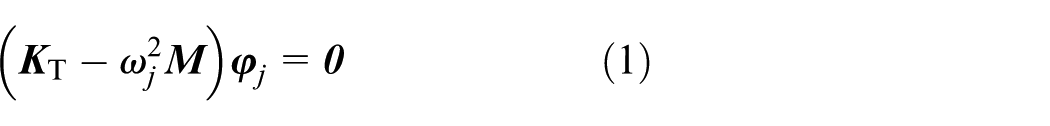
where
For tensile structures, the tangent stiffness matrix
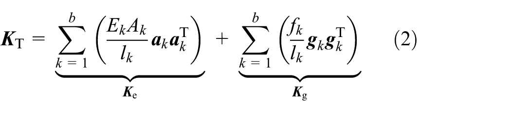
in which
Pretension deviation, defined as the difference between self-balanced member forces in the pre-stress state and the corresponding designed values, is a common issue in practice. Unlike rigid structures such as frames and shells, tensile structures are susceptible to pretension deviation due to the contribution of the geometric stiffness to the integral stiffness. During the service life of a large-span tensile structure, manufacturing and construction errors, creeping, base settlement, and cable sag can lead to geometric errors which are likely to alter the balanced configuration and self-stress modes. The major sources of geometric errors can be converted into element length errors during analysis. According to Deng et al.’s (2016) study on a cable-truss system as a stadium roof, the choice of tensioning schemes significantly affects control performance over pretension deviations. In the worst-case scenario, pretension deviations up to 48% were observed in the radial cables if all the members were passively installed with fixed lengths. The relationship between element length errors and pretension deviations can be described by an error sensitivity matrix. Chen et al.’s (2016) experimental study verified this theoretical approach and a peak deviation of 34.6% was reported. Unlike rigid structures such as frames and shells, tensile structures are susceptible to pretension deviation due to the contribution of the geometric stiffness to the integral stiffness. Under extreme loading conditions, pretension changes may lead to cable slack and severe stiffness degradation, or possible damage due to overstress. Therefore, the pretension state and integral stiffness of a tensile structure must be monitored for structural safety.
Large-scale structural systems such as tensile structures usually consist of a substantial number of members that are difficult to monitor or manipulate simultaneously. Conventional cable force measurement techniques such as the electro-magnetic (EM) method that requires installation of transducers on individual members consume time and effort and have high maintenance costs. In view of these difficulties in comprehensive pretension monitoring, researchers tried to find solutions from dynamic testing methods, which are widely applied to tension measurements of tie-rods (Gentilini et al., 2013) and stay cables in bridge engineering (Fang and Wang, 2012). Wu et al. (2017, 2018a, 2018b) proposed testing and evaluation methods for key stiffness based on targeted modal information, and also developed a modal identification method using optimizing step excitations to address the common issues of closely spaced modes in spatial structures.
However, step excitations by the sudden release of hanged loads are not suitable for as-built structures under usage. Furthermore, the excitation directions are strictly confined by the working space. Oscillators are too heavy for light-weight structures to retain their dynamic characteristics. Force hammers cannot provide sufficient excitations for a full-scale structure. None of these testing methods can meet the requirements of on-line and long-term health monitoring.
Operational modal analysis
Among the state-of-the-art techniques of modal identification, only a few are suitable to large-span tensile structures in engineering practice. As discussed above, the foremost difficulty lies in finding an effective and convenient way to excite a massive structure. Collecting complete excitation data from such a complicated structure is another difficult challenge. Therefore, the conventional experimental modal analysis (EMA) are no longer useful. Instead, operational modal analysis (OMA) methods that require only response signals based on ambient or natural excitations have emerged and provide an effective solution to the aforementioned challenges (Reynders, 2012).
The existing OMA methods can be classified into three categories. One category comprises the frequency domain methods based on the estimation of spectral functions (such as the power spectral density (PSD) and frequency response function (FRF)) of stochastic response signals; these methods include peak picking, polynomial fitting, enhanced frequency domain decomposition (EFDD), and poly-reference least squares complex frequency domain (p-LSCF, also known as PolyMax), and so on.
A second category operates directly in the time domain. A variety of time-domain methods are based on different forms of free response signals derived by natural excitation (NExT) or random decrement (RD) techniques, such as the Ibrahim time domain, least squares complex exponent, Eigensystem realization algorithm (ERA), and autoregressive moving average (ARMA). Subspace identification technique, driven either by the stochastic response data (SSI-Data) or its covariance (SSI-Cov), provides a powerful tool for large structures with high model order. ERA can be regarded as a specific case of SSI-Cov, and both of them utilize a subspace technique to reduce the Hankel (or Toeplitz) signal matrix.
The third category refers to time–frequency domain methods (Perez-Ramirez et al., 2016), such as wavelet method and Hilbert–Huang transform. They extract both time and frequency characteristics from the data by multi-scale analysis or decomposition and have great potential in time-variant and nonlinear system identification. However, these methods cannot yet deal with large systems due to computation inefficiency.
Several statistical approaches and numerical optimization methods can be applied with the above three categories to enhance performance, such as Bayesian inference, maximum likelihood, and linear regression. Another branch of system identification besides OMA is based on model-updating, such as different extensions of least squares estimation and Kalman filtering. They first assume an initial mathematic model for the vibration structure and then update the system parameters based on the measurements to minimize a prescribed cost function. These model-updating techniques can skip modal information and estimate structural parameters directly (Huang and Yang, 2014; Zhou et al., 2012), but rely heavily on the accuracy of the analytical model.
OMA techniques already have wide applications in many large-scale structures such as long-span bridges (Reynders and Roeck, 2015) and high-rise towers (Zhang et al., 2016), and these were even integrated with real-time wireless monitoring systems (Whelan et al., 2009). Most of the existing vibration testing measures are based on acceleration signals, which require installation of accelerometers on the structures. Recently, vision-based contact-free vibration testing techniques have emerged for dynamic displacement measurement (Ye et al., 2013), and corresponding OMA methods have been proposed (Canio et al., 2011). These techniques provide a far more efficient testing approach for bridges and towers in that the effort of deployment is saved. However, field applications of these appealing techniques on large-span tensile structures have been rarely reported. One major reason is that tensile structures usually exhibit complex spatial behaviors and cannot be simplified by plate or beam models such as in bridges or towels. The substantial number of degrees of freedom (DOFs) also adds to the difficulty of modal identification.
This article compares four methods representative of the above in terms of their performance in modal tests. The four methods selected were PolyMax (Peeters et al., 2004, 2015), EFDD (Brincker et al., 2001; Gade et al., 2005), NExT-ERA (Caicedo et al., 2004), and SSI-Data (Kim and Lynch, 2012; Peeters and Roeck, 1999). The relevant theories and detailed implementation methods can be found in the corresponding references. This work aims to validate the OMA methods on comprehensive modal identification of large-span tensile structures and to provide solutions to the aforementioned challenges and suggestions for engineering practice.
Experimental methods
Herringbone-ribbed cable dome model
The modal tests were performed on a 10 m wide, 1:10 scaled model of a herringbone-ribbed cable dome (Dong and Liang, 2014) (Figure 1). This novel structure has a layout of vertical struts and diagonal cables that differ from that of conventional cable domes. Instead of sharing a radical plane with the ridge cables, the cables follow a chevron arrangement along the circumferential direction, which enhances the circumferential stiffness and overall stability of the cable dome. This design also introduces a zigzag pattern along the roof edge, which enriches the architectural appearance. All the joints and members were weighted in advance to obtain a precise estimation of the structural mass. The cable dome model was anchored on a stiff ring girder of the supporting frame, and model’s boundary condition can be assumed as fixed.
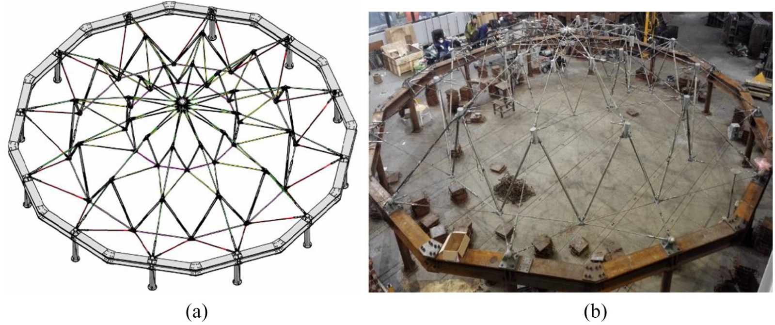
Herringbone-ribbed cable dome model with a scale ratio of 1:10: (a) 3D sketch and (b) physical model.
Preparation of tests
The cable dome model was erected as designed by actively stretching the diagonal cables at the outer-most and middle loops to the designed pretension level. Ridge cables, hoop cables, and diagonal cables at the inner-most loop and struts were regarded as passive members of fixed length. These members were placed on the scaffolding until the entire structure was elevated. A subset of the hoop cables, stay cables, and ridge cables were selected as passive cables to be monitored. Their cable forces were detected by force transducers installed directly on the members. The rest of the cables were measured by a portable dynamometer after stabilization. In addition, the coordinates of control nodes were scanned by a total station theodolite to capture and record structural displacements.
After the construction, the spatial coordinates of upper layer joints were collected to reconfirm the structural configuration. Measurement data showed that the upper layer of the cable dome model was basically erected to the designed position. Vertical coordinates of the observed nodes were less than 3 cm away from the design values. Cables forces were also measured and compared with the design values. Any active cables that exhibited large deviations were fine-tuned after the pre-tensioning construction. The deviations in passive members, however, were not treated. Except for several passive members like diagonal cables at the inner-most loop, major cables including ridge and hoop cables exhibited pretension levels that were very close to the designed condition. Therefore, the model was considered to be stretched to the designed pre-stress state.
More detailed information and a static loading experiment of the test model can be found in the cited reference (Liang et al., 2017). The static behaviors of the test model were shown to be in good agreement with the theoretical results. This scale model is representative of its full-scale prototype as well as the original design, with respect to the static performance.
The dynamic testing system consisting of excitation sources, accelerometers, and a high-speed data-acquisition instrument was then deployed onto the structure. Altogether five triaxial accelerometers and nine uniaxial accelerometers were used in the tests. The measurement devises and their features are listed in Table 1.
List of testing devices.

IEPE: Integrated Electronics Piezo-Electric; F.S.: Full-scale; rms: root mean square.
Optimal sensor placement regarding geometric stiffness
In structural modal tests, the number of measurement channels is usually far less than the number of structural DOFs because of equipment limitations. Therefore, sensor placement that helps to obtain adequate modal information has become an important issue for modal testing. Toward this objective, researchers have proposed various optimization criteria for sensor placement. Some criteria emphasize the identification effect. For example, the effective independence (EI) approach (Kammer, 1991) is based on the claim that the optimal case should guarantee mutual independence of the identified modes; the modal kinetic energy (MKE) approach insists that sensors be placed on DOFs that contribute the most to the modal kinetic energy, and the average acceleration amplitude (AAA) approach focuses on the quality of measurement signals. These criteria can be easily compounded to yield more thorough considerations, such as EI-MKE and EI-AAA (Liu et al., 2013). Some researchers maximized the damage sensitivity and minimized the noise sensitivity in the measurement selection to enhance damage identification performance (Xia and Hao, 2000; Zhou et al., 2013). Other optimization strategies tend to approach the optimal solution using numerical methods, such as genetic algorithms (Yao et al., 2012), neural networks, and others.
Taking EI-MKE as an example, the optimization criteria are based on a priority sequence vector defined as

where
Rearranging the DOFs according to the vector

where
Replacing

Major deformation patterns indicating the optimal sensor placement: (a) circumferential, (b) overall vertical, (c) global fluctuation, and (d) component vertical deformations.
In tensile structures, loss of stiffness due to pretension deviation is a more likely source of danger to the structural safety than material fatigue or cable ruptures. Therefore, the main objective of modal tests can focus on the evaluation of geometric stiffness instead of integral stiffness. The optimization can be further refined by considering the contribution of geometric stiffness to the modes by extracting those modes where geometric stiffness contributes the most and forming a reduced modal displacement matrix
With the orthogonality of the mode shape vector, multiplying

Substituting equations (2) into (5), the modal stiffness can be rewritten as

where
To evaluate the proportion of geometric stiffness in the modal stiffness at the rth mode, the following stiffness projecting factors are defined (Xia, 2014)
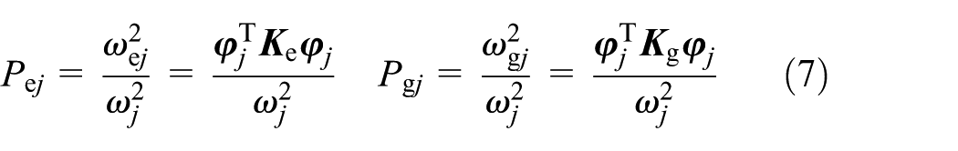
Rearranging the modes according to the geometric stiffness projecting factor vector
Figure 3 clearly shows that only in the first 15 modes (except modes 4 and 5) is the geometric stiffness the dominant contributor to the modal stiffness. The high-order modes mainly provide information about the elastic stiffness, which depends on the topological relationship, material properties, and structural dimensions, rather than cable pretentions. Therefore, this analysis focuses on only the first 15 modes for cable force identification.

Elastic and geometric stiffness projecting factors.
In this special case, the optimal schemes with and without the geometric stiffness refinement do not differ significantly. The placement scheme shown in Figure 4 was adopted for the complete structure. To obtain the most complete integral structural modal information as possible, after a set of tests, the sensors were moved to the adjacent trusses for another set of tests, retaining the positions of the reference node and the three channels on the central node. The reference channel was selected based on the principle that the modal displacement at the node remained sufficiently observable in the first 15 modes. The sensor placement scheme was thereby rotated counter-clockwise by 15°. This operation was repeated twice, and the three sets of sensor placement schemes were named Complete-A, Complete-B, and Complete-C. With these three sets of measurements, almost all the DOFs of interest were observed. Although the vertical vibrations of the outer-most hoop cable nodes were not monitored, the corresponding motion could be derived from the lateral movement of the adjacent ridge nodes based on their geometric relationship.
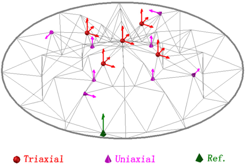
Optimal sensor placement for the complete structure (Complete-A).
In addition, a spatial cable truss within the cable dome was selected as a substructure. Sensors were intensely arranged on this substructure to obtain detailed measurements for the comparative study, as shown in Figure 5. As long as the analytical model is accurate and reliable, the stiffness of the substructure can be estimated through model-updating (Weng et al., 2013) or minimization of modal dynamic residuals as Zhu et al. (2016) implemented on a space frame bridge.
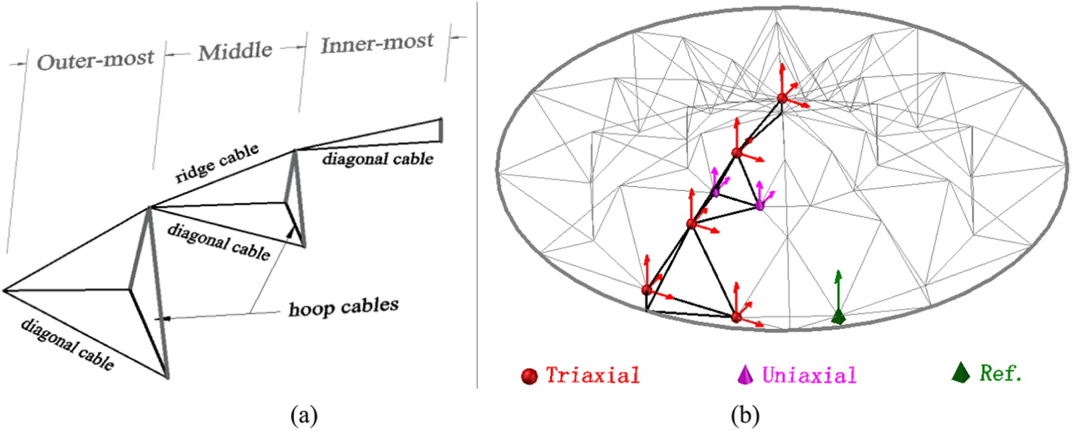
Optimal sensor placement for the substructure: (a) schematic of a cable-truss substructure and (b) sensor placement.
Dynamic testing protocol
These modal tests were conducted to compare the various methods in the following respects:
Excitation method. In this test, environmental excitation was simulated by random strikes at random locations using rubber hammers. Such excitation methods were used in both integral tests and substructure tests. On the substructure, a set of impact tests were also conducted using a testing hammer, and the excitation signal was recorded.
Complete structure and substructure. In view of the limitation on sensor channels, the authors followed two different strategies of modal testing: one strategy repeated the integral tests with different sensor placements on the complete structure and the other focused on substructure measurements.
Different pretension distributions. To investigate the susceptibility of structural stiffness to pretension deviation, several cables were manually loosened to half their designed pretension levels in separate modal tests. These tests aimed to determine the relationship between the structural modes identified and the known cable force distribution. Each test was tagged with an ID as shown in Table 2.
Testing schemes on the cable dome model.
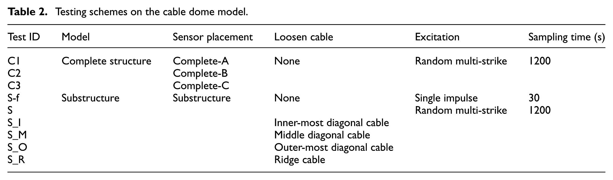
Table 2 also presents each of the dynamic testing protocols. In all tests, the sampling frequency was set at 1000 Hz, although 100 Hz can satisfy most cases. The higher frequency was selected to enhance the sample number for averaging without largely increasing the sampling time. Before conducting modal identification techniques, the data were down-sampled to 100 Hz to attenuate the high-frequency components.
Test results and modal analysis
Modal identification based on the test data of the complete structure and substructure were conducted via four commonly used OMA techniques: PolyMax, EFDD, NExT-ERA, and SSI-Data.
When using frequency domain methods, Hanning windowing was established, and the overlapping rate of averaging was set at 50%. For NExT-ERA, the parameters for the dimensions of Hankel matrix
Stabilization diagrams were employed to remove the spurious modes from the true structural modes. The convergence criteria were as follows: 0.01 Hz for frequency; 0.1 for damping; and 1% for mode shape based on the modal assurance criterion (MAC) value. When all convergence criteria were met as the model order increased, the corresponding mode was considered stable. After analysis, 82, 66, and 92 were selected for the PolyMax, ERA, and SSI system orders, respectively.
Test results of the complete structure
The identified frequencies f and damping
Modal identification results of the complete structure in the pre-stressed state.
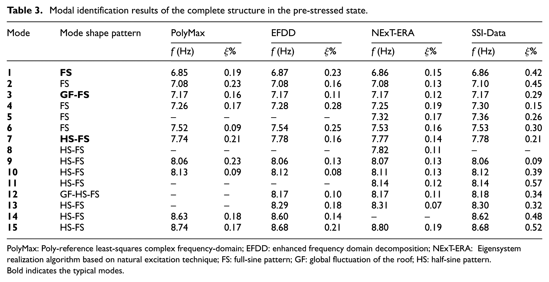
PolyMax: Poly-reference least-squares complex frequency-domain; EFDD: enhanced frequency domain decomposition; NExT-ERA: Eigensystem realization algorithm based on natural excitation technique; FS: full-sine pattern; GF: global fluctuation of the roof; HS: half-sine pattern.
Bold indicates the typical modes.
Despite their similarities, some modes identified by one method were not recognized by the others, such as Mode 8 identified by the ERA method. With a limited amount of data, all methods were challenged to identify closely spaced modes, which is common for massive structures characterized by a certain degree of symmetry. Many modes with very close frequencies but irrelevant mode shapes were identified at the expense of sampling time and data size, and there were inevitably some other modes that were not identified. Fortunately, several typical modes were well detected, as shown in Figure 6.
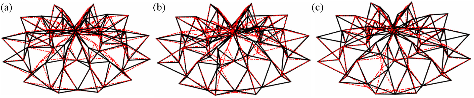
Typical modes identified from the complete structure: (a) Mode 1 (6.85 Hz), (b) Mode 3 (7.17 Hz), and (c) Mode 7 (7.74 Hz).
The first several modes mainly involved lateral vibrations of the spatial cable trusses. These modes revealed the lack of lateral stiffness of the structure due to the circumferential members missing from the top layer, in comparison with the traditional Geiger cable dome. The second typical mode showed a global fluctuation deformation pattern. Starting at approximately 7.77 Hz, some of the cable trusses presented a full-sine deformation pattern (see Figure 6(c)), instead of the half-sine pattern exhibited throughout the first six modes. In the higher-order modes, more local deformations of cable trusses were observed.
Damping results from different methods varied significantly and could only serve as criteria for modal stabilization. Prior researchers have found that damping properties in tensile structure are insignificant compared to those in traditional structures like frames and shells (Feng et al., 2011), and are therefore not of concern.
Although the four OMA methods used in this test have succeeded in identifying the major modes, they exhibited some differences in identification performance. Compared to the other three methods, EFDD was faster and more straightforward, but required manual selection. The time-domain methods omit a few modes that identified by the frequency-domain methods. SSI-Data was more time-consuming compared to NExT-ERA and PolyMax, but provided better stabilization diagrams, and thus is more suitable for automatic identification.
Test results of the substructure
Centralized testing provided better performance because of the denser sensor arrangement. Table 4 shows agreement among the identification results from the three different OMA methods and one EMA method: the least squares frequency domain (LSFD) method based on full FRF matrix obtained via the multi-reference impact technique (MRIT). More complete structural modes were identified at the expense of testing resources. The comparison shows that OMA methods based on output-only data performed almost as well as the laborious EMA method, which requires response and excitation signals in all DOFs. Although the OMA methods missed a few modes, they nonetheless succeeded in identifying all the typical modes of concern.
Modal identification results of the substructure in the pre-stressed state.

EMA: experimental modal analysis; LSFD: least squares frequency domain; OMA: operational modal analysis; EFDD: enhanced frequency domain decomposition; NExT-ERA: Eigensystem realization algorithm based on natural excitation technique; SSI-Data: Data-driven stochastic subspace identification; FS: full-sine pattern; GF: global fluctuation of the roof; HS: half-sine pattern.
Bold denotes the typical modes.
As shown in Figure 7, the first mode shape clearly exhibited the half-sine lateral deformation of the cable truss. Mode 3 showed a vertical deformation inherited from the global fluctuation of the complete structure. Mode 7 presented another local lateral deformation but with a full-sine pattern instead.

Typical identified modes of the substructure: (a) Mode 1 (6.83 Hz), (b) Mode 3 (7.17 Hz), and (c) Mode 7 (7.76 Hz).
Sensitivity of modes to pretension deviations
Table 5 compares the test results for different pretension deviation distributions, and the results show that the structural modes change only slightly when the individual cable force decreased. Most of the frequency differences caused by pretension loss in individual members were within 1%. One explanation for this result is that the structure contains a large number of members and most individual members have limited influence on the overall structure (except for highly sensitive members like hoop cables). Another explanation is that the experimental model exhibits larger elastic stiffness than ideal cable-strut models, and therefore, the geometric stiffness is relatively less significant. The global modal information given by this test model is not sufficiently sensitive to obtain precise readings on individual cable forces.
Identified modes of the substructure with different pretension deviations.

Italic indicates a difference in mode shape although the frequencies are close; bold indicates the typical modes.
Discussion
Comparison between theoretical and experimental modes
The theoretical analyses of tensile structures in the literature are mostly based on a line model consisting of cable and strut elements only. According to the comparison between theoretical and experimental results, the test model appeared stiffer compared to the ideal model and exhibited higher frequencies. Because the structural mass was precisely evaluated, the major factors responsible for the modal differences could be concluded to be as follows:
Moment resistance of cables. Unlike the cable elements in the ideal model, the ridge cables and hoop cables are in fact continuous cables that have bending stiffness. The pinned-cable assumption in the ideal model may underestimate the lateral stiffness of a cable truss.
Dimensions of joints. For simplicity, the connections of members in the ideal model are usually assumed to be zero-sized, whereas in reality, the joint is more of a rigid body with non-negligible size. Therefore, the actual effective length of members is shorter than that in the line model, leading to higher element stiffness.
Rigidity of connections. In the ideal tensile structure model, the connections among members are assumed to be moment-free, whereas in reality, such connections are usually implemented with one-dimensional pin connections, which exhibit rotational rigidity along the other two axes. Details and orientation of these connections, as well as mechanical locking, add to the complexity of modeling.
Mechanical friction. Because of fabrication and construction errors, the model will not be properly installed without coercive assemblage actions. Together with the applied pretension, the structural model stored a certain level of pre-stress, which was accompanied by mechanical frictions at each connection, increasing the structural damping and stiffening the structure.
Natural frequencies of different models (Hz).

FE: finite element.
Bold indicates the typical modes.
Any of these factors may introduce additional stiffness to the structure. Taking the first two factors into consideration, different finite element models (FEMs) have been constructed and their natural frequencies are compared in Table 6. Model A refers to the ideal cable-truss structure: ridge and hoop cables are modeled as continuous beams in Models B and C. The effective lengths of members are modified in Model C by modeling the joints as rigid solid bodies. Although these modifications significantly enhanced the natural frequencies, they still do not precisely match the test results. Factors 3 and 4 are difficult to model due to their complexity and randomness, but they have non-negligible impacts on the structural stiffness. In conjunction with the size effect, the above problems also exist in full-scale tensile structures because the connection details for both the test model and real structures are very similar.
The first mode in the FEM results was not identified in the test results, because the first mode involves simultaneous lateral leaning of all cable trusses, which is difficult to trigger by simple artificial excitation. Pretension deviation is also a major reason for some of the missing theoretical modes, and the deviation also induces unexpected modes, because it breaks the symmetry and periodicity of the ideal structure.
The difference between the theoretical and experimental modes is even more significant than that caused by pretension deviation of individual members. Therefore, no easy method yet exists to identify cable forces directly from global modal information and FEM analysis, unless a numerical model can be established that describes the real structure in minute detail.
Fortunately, the modal identification accuracy is sufficiently good to capture the modal difference between cable trusses, which helps to locate cable slackness or overstress as long as the global pretension remains at the designed level. Changes in global mode shapes also help in diagnosing stiffness degradation in substructures. Standard modes can be obtained by pre-calibrating one cable truss with precise measurements of cable forces, and thus, pretension deviations in other cable trusses can be detected by modal comparison.
Identification of pretension loss
Pretension loss of the cable structure results in the degradation of global and local stiffness, which can also be regarded as a form of structural damage. A damage identification technique can detect pretension loss in the structure as long as technique’s sensitivity is adequate. Modal parameters are sensitive to the members that contribute most to the geometric stiffness, and vice versa.
Given the modal information, a damage index based on modal strain energy (MSE), such as the MSEBI proposed by Seyedpoor (2012), can be adopted to pinpoint the elements upon which damage occurs. Theoretically, as the elemental stiffness decreases, the average elemental MSE over the overall structural MSE increases. For cable structures, this index can be further optimized by excluding the elastic stiffness irrelevant to cable pretension.
The modal geometric strain energy (MGSE) before and after damages occur is defined as follows
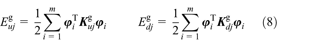
in which
The new index

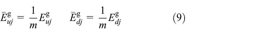
Theoretical results from the modal analysis of ideal structures before and after loosening ridge cable 12 (one of the ridge cables at the outer-most loop) verify this method. Pretension deviation and the corresponding MGSEBI of all the ridge cables at the outer-most loop are shown in Figure 8(a). The index clearly indicates pretension loss in ridge cable 12.
MGSEBI of ridge cables when cable 12 is loosened: (a) theoretical model and (b) experimental model.
The above presented damage detection approach requires sufficient modal information of the structure, which is usually unrealistic in practice, especially for massive structures. As concluded from the previous section, the identified modes before and after damage may not easily match. As a result, the MGSEBI derived directly from the test data cannot precisely reveal the damage position.
To guarantee the detection accuracy, the mode shapes between tests should be matched and coupled first according to MAC values. A tolerance value

The MGSEBI was then calculated from the subset of identified modes
Key issues on field applications
The experimental methods presented above may encounter several critical issues when applied to real structures. These issues are as follows:
Deployment of the testing system. Wiring a decentralized system on a large-span structure is laborious and expensive, and it will generate electronic noises if the sensors are not equipped with analog-to-digital converters. Therefore, a wireless sensing system is a better option for field deployment. However, most of the OMA methods require continuous sampling over a period of time to capture adequate and distinguishable signals, so as to guarantee the identification accuracy. Battery life and package loss during transmission are major challenges for wireless systems in this application.
Signal quality. Unlike the multi-strike excitations in this experiment, ambient excitations are much weaker while the noise sources are more complicated. It is important to enhance the signal-to-noise ratio through noise suppression measures and high-quality instruments.
Operating conditions. For many large-scale structures such as bridges and towers, strong winds (and even typhoon) are desirable conditions for ambient testing in that the response signals are strong. The measurement data can also be used to model wind characteristics for other research purposes (Ye et al., 2017). However, the performance of OMA techniques and identification methods may not be good for tensile structures, as the configuration and pretension distribution of the structure will change due to large deformation under strong wind loads. The modal testing is suggested to be performed under moderate loading conditions.
Influence of sheeting diaphragms. When applied as a roofing system, tensile structures are likely to be strengthened by purlins and sheeting diaphragms. The additional stiffness may compensate for the stiffness degradation caused by the potential pretension loss, and thus, affects the identification performance. Furthermore, aerodynamic damping of the membranes may significantly increase the structural damping, which was reported to vary between 0.15% and 1% for bare tensile structures (Cao and Xue, 2008), and may amplify the wind-induced fluid–solid interaction effect.
Conclusion
This article presents a series of modal tests on a 10-m-span cable dome structural model and compares different testing protocols and various modal identification methods. The following conclusions were drawn from the results.
A revised optimization method for sensor placement was proposed to improve the measurement of the geometric stiffness. The proposed method was found to overcome the sensing equipment limitations and enhance the modal identification performance.
By applying multiple hammer strikes at random locations, the modal tests simulated the environmental excitations. With output data only, the major modes of the integral cable dome structure and substructure were successfully identified. The test results also validated existing OMA methods such as PolyMax. EFDD, NExT-ERA, and Data-SSI on the cable dome model.
Pretension deviations in individual members were found to have detectable influence, though not sufficiently significant for precise reading, on both the natural frequencies and the mode shapes of the typical modes. Stiffness degradation positions could be identified by mode shapes from decentralized testing. A modified MGSEBI method was proposed to detect pretention loss, and the method was verified by the test results. Further investigation can be conducted via localized testing on the tagged substructure.
The identified modes from the test data suggest greater stiffness in the test model than in the theoretical model. With regard to dynamic behaviors, the ideal cable-truss model does not guarantee simulation accuracy for tensile structures. Modification of the analytical model to enhance detail, though complicated, is required for precise pretension identification from modal characteristics of the test model.
Footnotes
Acknowledgements
Special thanks are extended to Jiangsu Donghua Testing Technology Co., Ltd. of China for the use of their instruments.
Declaration of Conflicting Interests
The author(s) declared no potential conflicts of interest with respect to the research, authorship, and/or publication of this article.
Funding
The author(s) disclosed receipt of the following financial support for the research, authorship, and/or publication of this article: This work was supported by the National Natural Science Foundation of China (Grant Number 51478420).