Shear resistance estimation for unreinforced masonry walls based on Gaussian process models

Abstract

Uncertainty results in misestimate of the shear resistance of unreinforced masonry walls. The misestimate is difficult to correct using deterministic calculation models even when sophisticated numerical models are used. To address this issue, the authors converted the deterministic calculation models for shear resistance of unreinforced masonry walls into prior Gaussian process models and then collected experimental results to train the prior Gaussian process models. They evaluated the resultant posterior Gaussian process models and found two of them are preferable. The two favorable posterior Gaussian process models can well interpolate the collected experimental results and can predict the shear resistance of the unreinforced masonry walls in the authors’ experiments with full information. The interpolation and predication demonstrate that the posterior Gaussian process models can combine and weight prior engineering judgments and observational information from experimental results and then can quantitatively specify the remaining uncertainty of the estimation. In addition, the Gaussian process models are efficient, favorable for reliability analysis, and easily improvable. Therefore, they are potentially useful in engineering practices.

Keywords

estimation Gaussian process shear resistance uncertainty unreinforced masonry wall

Introduction

Unreinforced masonry (URM) walls are principal structural elements in masonry structures that have been widely used around the world. An appropriate estimation of the walls’ resistance is critical for safety assessment of the masonry structures, and for potential strengthening design of them. Most URM walls are supposed to resist shear force under vertical compression. Therefore, shear resistance estimation for URM walls under compression is essential and has attracted considerable research attention in decades (Binda et al., 1991; Dhanasekar et al., 1985; Mazzotti et al., 2014; Page et al., 1980; Shing et al., 1990; Zhu et al., 1980).

Extensive physical experiments have revealed that the URM walls’ shear failure is subject to a wide range of parameters, and it can happen in different modes. Some influential parameters are difficult—if not impossible—to quantify comprehensively (Sutcliffe et al., 2001; Tomaževič et al., 1996). Therefore, to estimate the shear resistance deterministically is difficult. The URM walls are highly heterogeneous, because the units and the mortar have different mechanical properties and they combine in different bricklaying patterns (Grimm, 1988; Mojsilović and Stewart, 2015). The heterogeneity results in unpredictable orientation of principal stresses with respect to bed mortar joints and then causes uncertain damages of the unit–mortar interfaces (Vasconcelos and Lourenço, 2009). Moreover, the units and the mortar joints decay at different paces. Deficiencies can randomly arise within them or at their interfaces during use. These deficiencies irregularly impair the URM and reduce the URM walls’ shear resistance in a random way (Gentilini et al., 2015). There are experimental results show that the URM walls are not perfectly elastic even in the range of small deformation (Sutcliffe et al., 2001). Under coupling interaction of shear and flexure mechanism, the walls may fail in diagonal shear mode, rocking modes with toe crushing, flexure modes with toe crushing, sliding mode, or mixed modes, displaying very different resistance (Shing et al., 1990). All the failure modes are brittle, especially when the vertical compression is high, and then to measure the resistance exactly is not easy (Konthesingha et al., 2013; Mojsilović et al., 2010). Loading pattern and boundary conditions also have significant impacts on the shear resistance of the URM walls (Gams et al., 2017; Tomaževič et al., 1996). For example, the repeated compressive loading can cause significant reduction in resistance (Nazar and Sinha, 2007a). In addition, the URM walls’ shear resistance is influenced by some retrofitting measurements, like grouting or mortar joint reinforcement (Bolhassani et al., 2016; Schultz et al., 1998). The extensive experimental results indicate that the shear resistance is far from deterministic: the coefficient of variation (COV) of the experimental results for mechanical properties of URM can be higher than 0.25 (GB50003-2011, 2011). The shear resistance estimation under such a high variation could be unreliable. To reveal the shear failure mechanism underlying the huge volume of experimental results, extensive study has been focused on resistance calculation models for URM walls, including numerical models and analytical models.

The numerical models attempt to represent the walls’ failure mechanism comprehensively. They can be classified into three categories according to their level of detail, that is, microscopic models, mesoscopic models, and macroscopic models (Lourenço, 1996; Roca et al., 2010). The microscopic models treat the units, the mortar, and the unit–mortar interfaces separately and then calculate the walls’ responses under different loading cases (Lourenço, 2010). They are often complicated because different elements have to be combined (Kalliontzis and Schultz, 2017). The mortar joints can be simulated by interface elements that represent bonding and frictional contact (Snozzi and Molinari, 2013); the units can be simulated using solid elements that dynamically interact with each other through collision (Lemos, 2007). The detailed microscopic models require a careful—but potentially subjective—selection of material models and many input parameters (Calderón et al., 2017), and they take much computational time to capture the development of intrinsic damages in the URM. During their calculation, high local stresses and stress gradients often result in divergence (Ali and Page, 1989). The explicit method can be used to address the divergence issue, but it might take much more computational time (Noor-E-Khuda and Dhanasekar, 2018).

The mesoscopic models homogenize the URM into continuum and then calculate the URM walls’ resistance (Lourenço et al., 2007). Direct mesoscopic strategy is only appropriate under very small loads because it neglects the heterogeneity and existing damages in the URM (Peralta et al., 2016). To appropriately homogenize the URM, displacement boundaries should be applied on a representative volume element (RVE) consisting of units and mortar, and then equivalent overall material properties should be determined by integrating stresses and strains responses over the RVE (Ma et al., 2001). For the homogenized URM, different failure criteria can be imposed, including the Hill–Rankine criteria (Janaraj and Dhanasekar, 2014), the Mohr–Coulomb criteria (Bruggi and Milani, 2015), and the Drucker–Prager criteria (Köksal et al., 2013). Under cyclic loading, stress–strain curves of the homogenized URM can be represented by normalized polynomial functions (Nazar and Sinha, 2007b). However, to justify the calculation results of the mesoscopic models, parameters of the failure criteria and stress–strain curves might have to be adjusted subjectively (Orduña and Lourenço, 2003).

The macroscopic models treat the URM walls or their portions as super elements. The super elements can be regarded as rigid, and the nonlinearity deformation is concentrated in predefined contact regions around them (Costa et al., 2015). The nonlinearity deformation can also be represented by normal springs and shear spring connecting the super rigid elements, and the mechanical characteristics of the springs are defined considering the mechanical properties of mortar (Peng et al., 2018). The macroscopic models can simulate the extreme responses of masonry structures, including buckling and collapse (Casolo, 2004). However, they are more effective in simulating the global responses of the structures under dynamic inputs, than in simulating the local responses within an URM wall under static loads (D’Ayala and Shi, 2011).

In general, the numerical models require much time for modeling and calculation. They resort to different elements, solution procedures, constitutive laws, and failure criteria (Costa et al., 2015; Nazar and Sinha, 2007b). For the complicated constitutive laws and failure criteria, not all parameters have clear physical meanings, and some of these parameters are difficult to measure (Tomaževič and Weiss, 2010). Moreover, the mechanical parameters of the URM vary from wall to wall, and the parameters set for any specific constitutive laws and failure criteria will not generally be appropriate. Therefore, the numerical models that heavily depend on the parameters introduce uncertainty into their calculation results potentially.

As an alternative to the sophisticated numerical models, the analytical models proposed in design codes have simple forms, and they ensure the safety of the URM walls with considerable margin (ACI 530-05, 2005; EN 1996/Eurocode 6, 2005; GB50003-2011, 2011; Theodossopoulos and Sinha, 2013). They are efficient because they impose strong simplifications on mechanical parameters and failure modes. However, the simplifications make them less flexible than the numerical models in representing different failure mechanisms (Brunner and Shing, 1996) and less accurate in terms of the agreement between their results and the experimental results (Haach et al., 2013; Tomaževič, 2009). The analytical models are often biased because their parameters are conservatively chosen to ensure the safety margin (Schultz et al., 1998). In some circumstances, the strength of URM is set to be half or less of the experimental average (GB50003-2011, 2011; Hendry, 1982). Such a high reduction neutralizes the efforts to optimize the calculation models, and it could mislead the structural assessment, reliability analysis, and maintenance of the target URM walls (Haukaas et al., 2011).

The shear resistance estimation for URM walls has not been well addressed with the extensive experimental results and the available calculation models. The calculation models hardly reproduce the experimental results systematically without repeated adjustment of the input parameters (Sui, 2007; Torres et al., 2017), and they cannot systematically evaluate the differences between their results and the experimental results (Haukaas et al., 2011). Consequently, either overestimation of the resistance that leads to insufficiently interventions and inadmissible risks, or underestimation of the resistance that leads to over-strengthening or unnecessary loss, can happen. The reason for these issues is the conflict between the uncertain nature of the shear failure and the deterministic forms of the calculation models (Atamturktur et al., 2012). The uncertainty has been acknowledged and some counter measures have been proposed. For example, Eurocode 8 introduces a confidence factor (CF) to represent the influence of model uncertainties (Rota et al., 2014). Its value depends on the knowledge level (KL) obtained on the geometry, on the structural details, and the mechanical characteristics of the materials (Clementi et al., 2016).

Both parameter uncertainty and model uncertainty exist in the estimation of the shear resistance of the URM walls. The parameter uncertainty results from the significant aleatory randomness of the mechanical properties of the heterogeneous URM, and also from the observational error in the experimental results. Such strong uncertainty makes it unjustified to estimate the parameters on the basis of simple statistical moments over the limit observational samples (Ang and Tang, 1975). The shear resistance estimation relying on the insufficiently evaluated parameters could be unreliable (Dymiotis and Gutlederer, 2002; Ellingwood, 1981). The mechanical parameters of masonry are not only uncertain but also correlated with each other. For example, a variety of the geometry of the units results in a mismatch between the units and their surrounding mortar joints. This mismatch leads to complicated stress states in the URM and then uncertainly impairs the strength. A lack of information about the correlations among the mechanical parameters introduces even more severe uncertainty. Therefore, we might have to estimate the shear resistance of URM walls with the significant parameter uncertainty.

Besides, there is the model uncertainty that results from the imperfections of the calculation models. Influenced by the uncertain and correlated parameters, the shear failure of the URM walls under compression is a very complicated procedure. To predict the failure mode of a wall before loading—and then to choose a specific resistance calculation model in advance—is not realistic because of the strong uncertainty. Meanwhile, a generally accepted calculation model that can comprehensively represent all uncertain parameters and the complicated failure mechanisms has not been developed yet. As a result, both the numerical models and the analytical models have to represent the real URM walls in idealized or simplified ways. To achieve such idealization, the former ignore some influential parameters and the latter assume particular failure mechanisms. They are all biased because of the idealizations. Therefore, we might have to estimate the shear resistance of URM walls, even we cannot represent the shear failure procedure correctly.

We face the uncertainty as a major issue in shear resistance estimation for the URM walls, also in appropriate strengthening design for the walls (Colonna et al., 2017; Como, 2014). This issue can be addressed by explicitly accounting for the uncertainty, through modeling the shear resistance as a stochastic process over the uncertain parameters and models (Soize, 2013). The Gaussian process (GP) model and the artificial neural network (ANN) are effective in doing so. The two methods are popular in the field of machine learning, and they have strong relations and could potentially give similar results (Neal, 1996). It has been reported that the ANN can effectively reproduce experimental results for shear resistance of grouted reinforced concrete masonry walls (Zhou et al., 2017). The GP model is simpler and more transparent than the ANN (Rasmussen and Williams, 2006). Using the GP model, we can use plausible calculation models as priors to represent the engineering judgments and then use available experimental results to train the priors. The resultant posterior GP models retain the engineering judgments from the priors and use them to avoid relying completely on the scattered experimental results with inherent errors. This feature potentially relieves the parameter uncertainty. Meanwhile, the GP models represent the engineering judgments just vaguely and let the experimental results “speak” sufficiently for themselves. Thus, they relieve the bias of the priors and then relieve the model uncertainty. The GP models automatically combine and weight the engineering judgments from the priors and the observational information from the experimental results. They provide estimation with complete information and can quantitatively specify the remaining uncertainty.

Unlike the numerical or analytical models, the GP models define a purely mathematical relationship between the inputs and the outputs while disregarding the involved physics. They do not have divergence issues or heavy time burdens. Therefore, they can be efficient surrogates to the numerical or analytical models (Atamturktur et al., 2012). More importantly, they allow us to estimate starting from a biased prior model that is not mechanically sound. The situation happens in many real-world practices, because our knowledge of the parameters, the real states, and the failure mechanism of the target masonry walls is vague generally.

In this study, we converted the deterministic shear resistance models of URM walls into prior GP models, and then trained and updated the prior GP models based on available experimental results. We estimated the shear resistance of URM walls using the updated GP models and then verified the estimation. The rest of this article is organized as follows. In section “Experimental results and calculation models for shear resistance of URM walls,” we collect experimental results and introduce three deterministic calculation models for shear resistance of URM walls. In section “GP models for shear resistance of URM walls,” we explain the GP modeling procedure that uses the deterministic calculation models as priors. In section “Shear resistance estimation based on the GP models,” we establish GP models for shear resistance of URM walls, train the GP models using the collected experimental results, and then verify their interpolation and predication ability. In section “Conclusion,” we summarize the research findings and point out the potentials of the GP models in engineering practices.

Experimental results and calculation models for shear resistance of URM walls

Experimental results

The extensive physical experiments for shear resistance of URM walls have accumulated a huge volume of results. These results were obtained under different conditions and they are significantly scattered. Their inherent uncertainty should be addressed before they can be used in the estimation of the shear resistance.

We collected 78 sets of experimental results from literature, as shown in Appendix 1. To reduce potential bias caused by the difference in material properties, only the results for brick URM walls were collected. Some values in Appendix 1 were converted from the original parameters in the literature.

Although the collected results are not complete, they can be used to explain the GP modeling and estimation procedure. Other experimental results can be incorporated easily following the same procedure.

Calculation models

Although deterministic calculation models for shear resistance of URM walls do not explicitly account for the uncertainty, they convey important engineering judgments. Therefore, they contribute to relieve the uncertainty. We resort to three typical models as follows, which are widely used in real-world practices.

The first model is based on the Mohr–Coulomb failure criteria, and it specifies the shear resistance as a linear function of the cohesion and the vertical compressive force. The general form of the model is (GB50003-2011, 2011; Tomaževič, 2009)

R_{v} = A v_{0} + μ N

where $R_{v}$ is the wall’s shear resistance under compression, A is the wall’s cross-sectional area which bears the vertical compressive force, $v_{0}$ is the cohesion—or shear strength without compression—of the masonry, µ is the frictional coefficient, and N is the vertical compressive force.

In most practices, the cross-sectional area A can be well measured. Taking A to be deterministic and then dividing the two sides of the above equation by it, we obtain the following equation

τ = v_{0} + μ c

where $τ = R_{v} / A$ is the wall’s nominal shear strength under compression and it is a convenient indicator of the shear resistance of the wall in practices, and $c = N / A$ is the nominal compressive stress. Here, we save the common stress notation σ for the standard deviation in the following sections.

The second model is based on the maximum tensile stress theory, and it specifies the nominal shear strength as a nonlinear function of the cohesion and the nominal compressive stress. The general form of the model is as follows

τ = v_{0} \sqrt{1 + \frac{c}{v_{0}}}

The two above-mentioned models are applicable directly for ideal elastoplastic materials. For URM, calibration parameters have to be used to fit the models to experimental results. Then, the models become

τ = α v_{0} + β c

(1)

and

τ = α v_{0} \sqrt{1 + β \frac{c}{v_{0}}}

(2)

where α and β are the calibration parameters. Equation (1) is recommended by many design codes because of its simplicity, and thus, stability.

Most URM walls have irregular cracks that are difficult to model. To avoid the theoretical difficulty, we can establish the shear resistance model by a direct linear regression of enough shear–compression experimental results. Taking the low masonry cohesion as a constant, the regression leads to another simple model. The general form of the model is (ACI 530-05, 2005)

τ = α + β c

(3)

With different sets of calibration parameters, the above-mentioned models are considerably different from each other. Moreover, other plausible models that are not in the forms of equations (1) to (3) exist. The different models are not interchangeable because they refer to different failure mechanisms. However, when estimating the URM walls’ resistance in real-world practices, it is difficult to predict the failure mechanism of the target wall, and then it is difficult to choose a sound equation in advance. Using biased equations is not mechanically sound, but the situation happens. This is a source of uncertainty.

The bias can be relieved by trying to use models that are as appropriate as possible. However, the bias cannot be eliminated. If sophisticated numerical models were used, the relief of the bias might come with time burdens, potential divergence issues, and truncation errors in calculation. The errors add to the uncertainty when they accumulate through the iterative calculation procedures. Therefore, careful choosing or deliberate improvement of the deterministic models cannot address the uncertainty issue. We often estimate the shear resistance starting with the biased models.

To account for the uncertainty in the parameters and the models explicitly, we modeled the shear resistance as a stochastic process and converted the above-mentioned deterministic models into GP models, as discussed in the next section.

GP models for shear resistance of URM walls

A GP model describes a probability distribution over functions. It can specify the uncertain relationship between the output nominal shear strength $τ$ and the inputs v₀ and c. The GP model is flexible because it has vague requirements on how the functions look like. We can choose a function that we believe to be qualified to represent the plausible engineering judgments, and then we have a prior GP model. As the next step, we can train the prior GP model using available experimental results. Through the training, we combine the engineering judgments and the information from experimental results and then establish a posterior GP model within the Bayesian framework. The posterior GP model is a favorable base for estimating the nominal shear strength $τ$ , and it can be further updated whenever new experimental results are available.

Prior models

A GP model for the shear resistance of URM walls can be expressed as follows

τ (x) ~ N (m (x), C (x, x'))

(4)

where $N$ denotes the normal distribution, x is the input vector that contains the parameters $v_{0}$ and c, $m (x)$ is the mean function, $C (x, x')$ is the covariance matrix whose elements are the covariance functions, and $τ (x)$ is the output nominal shear strength. The functions become vectors for discontinuous inputs and outputs. The GP model is completely specified by its mean function and covariance functions.

Equation (4) denotes the conversion of the deterministic models if we set the prior of the $m (x)$ to be equation (1), (2), or (3). Although the equations are imperfect and biased, many masonry walls designed by following them are reliable. We can use the equations to compensate for insufficient information from the scattered experimental results. If the prior knowledge about the relation between the inputs and the outputs is not adequate, we can drop the mean function and use solely the covariance matrix $C (x, x')$ to determine a GP model. We numbered the GP models using equation (1), (2), or (3) as prior $m (x)$ by 1, 2, and 3, respectively, and numbered the GP model without a prior $m (x)$ by 4.

We specified the prior covariance functions, that is, an element in $C (x, x')$ , in a squared exponential form as follows (Rasmussen and Williams, 2006)

C (x, x') = σ_{f}^{2} \exp [- \frac{1}{2} {(x - x')}^{T} l^{- 2} (x - x')] + σ_{n}^{2} δ (x, x')

(5)

where $σ_{f}^{2}$ is the maximum allowable covariance between any two samples of $τ (x)$ , l = diag[l₁, l₂] is a diagonal matrix of distance scale factors that controls the smoothness of the model in each dimension of x , and $σ_{n}^{2}$ represents the observational error. Furthermore, $δ (x, x')$ is the Kronecker delta function; it equals to 1 if $x = x'$ , otherwise it equals to 0.

Equation (5) has favorable features. First, it quantitatively tells different uncertainty sources: the first term on the right side denotes the bias introduced using the prior mean functions, and the second term denotes the random observational errors. Second, it makes the model smooth: the closer the inputs, the more similar are the outputs. Along with the increase of $‖ x - x' ‖$ that is the distance between two inputs, the covariance $C (x, x')$ decreases subject to the distance scale factors l₁ and l₂. The l₁ and l₂ help to weight out the overcomplicated candidate models during model training. Third, it is flexible because it has the adjustable hyperparameters $σ_{f}$ , l₁, l₂, and $σ_{n}$ .

Using equations (1) to (5), we converted the deterministic models into stochastic GP models, which contain the calibration parameters $α$ and $β$ and hyperparameters $σ_{f}$ , l₁, l₂, and $σ_{n}$ . We can choose prior values for these parameters following our engineering judgments and then establish the prior GP models.

Training and updating of the prior models

The posterior values of calibration parameters $α$ and $β$ and hyperparameters $σ_{f}$ , l₁, l₂, and $σ_{n}$ . can be inferred by maximizing the log likelihood as follows (Hoff, 2009)

\log P (τ | x, θ) = - \frac{1}{2} τ^{T} C^{- 1} τ - \frac{1}{2} \log det (C) - \frac{n}{2} \log 2 π

(6)

where $θ = [α, β, σ_{f}, l_{1}, l_{2}, σ_{n}]^{T}$ and $C = C (x, x')$ . The input vectors x , the covariance matrix C , and the output $τ$ can be determined by available experimental results. The first term on the right side of equation (6) represents how well the experimental results are fitted, the second term penalizes the model complexity, and the third term is a log normalization term. The maximization of equation (6) results in parsimonious posterior models that combine and weight the prior engineering judgments and the information from the experimental results (Rasmussen and Williams, 2006). This procedure is fully Bayesian and is referred to as GP model training.

An important feature of the GP models is that the training can be triggered whenever new experimental results are available. The posterior GP models can then be further trained to incorporate more information from the new observations. To distinguish the training of the prior models and the further training of the posterior models, we refer to the latter as GP model updating.

Probability density functions of nominal shear strength

For any particular input $x^{*}$ , the output nominal shear strength $τ (x^{*})$ is still in the joint Gaussian distribution specified by the posterior GP model. Thus, we have the following equation

[\begin{matrix} τ (x) \\ τ (x^{*}) \end{matrix}] ~ N ([\begin{matrix} m (x) \\ m (x^{*}) \end{matrix}], [\begin{matrix} C (x, x) & C (x, x^{*}) \\ C (x^{*}, x) & C (x^{*}, x^{*}) \end{matrix}])

(7)

and we can further determine a normal probability density function (PDF) for the $τ (x^{*})$ as follows (Rasmussen and Williams, 2006)

\begin{matrix} τ (x^{*}) | τ (x) ~ N {m (x^{*}) + C (x^{*}, x) C {(x, x)}^{- 1} [τ (x) - m (x)] \\ C (x^{*}, x^{*}) - C (x^{*}, x) C {(x, x)}^{- 1} C (x, x^{*})} \end{matrix}

(8)

The normal PDF contains full information, including the engineering judgments and their biases, observational information from the experimental results, and the random observational errors. We can use the mean or an appropriate quantile of the PDF as an estimator of the nominal shear strength, and we can determine the confidence interval of such an estimator simultaneously. These advantages are not available when using deterministic models, individual experimental result, or simple statistics over a few experimental results. We explain the estimation procedure using some instances in the next section.

Shear resistance estimation based on the GP models

GP modeling

To establish prior GP models for the nominal shear strength, we judged the prior calibration parameters $α$ and $β$ according to available literature (ACI 530-05, 2005; GB50003-2011, 2011). In addition, we set the l₁ and l₂ to be the standard deviations of the $v_{0}$ and c in Appendix 1, respectively, and set both the $σ_{f}^{2}$ and $σ_{n}^{2}$ to be half of the variance of the $τ$ in Appendix 1.

The prior parameters are listed in Table 1, and the prior GP models are illustrated in Figure 1. Figure 1 shows that the collected experimental results are very scattered. If we tried to fit the relationships between the inputs and the outputs using deterministic parametric models, the models would be very complicated and then unstable.

Table 1.

Prior calibration parameters and hyperparameters.

Model	Mean function	Covariance function	Calibration parameters		Hyperparameters
Model	Mean function	Covariance function	α	β	$l_{1}$	$l_{2}$	$σ_{f}^{2}$	$σ_{n}^{2}$
1, Prior	Equation (1)	Equation (5)	1.00	0.19	0.29	0.52	0.01	0.01
2, Prior	Equation (2)		1.00	1.00	0.29	0.52	0.01	0.01
3, Prior	Equation (3)		0.25	0.45	0.29	0.52	0.01	0.01
4, Prior	None		–	–	0.29	0.52	0.01	0.01

Figure 1.

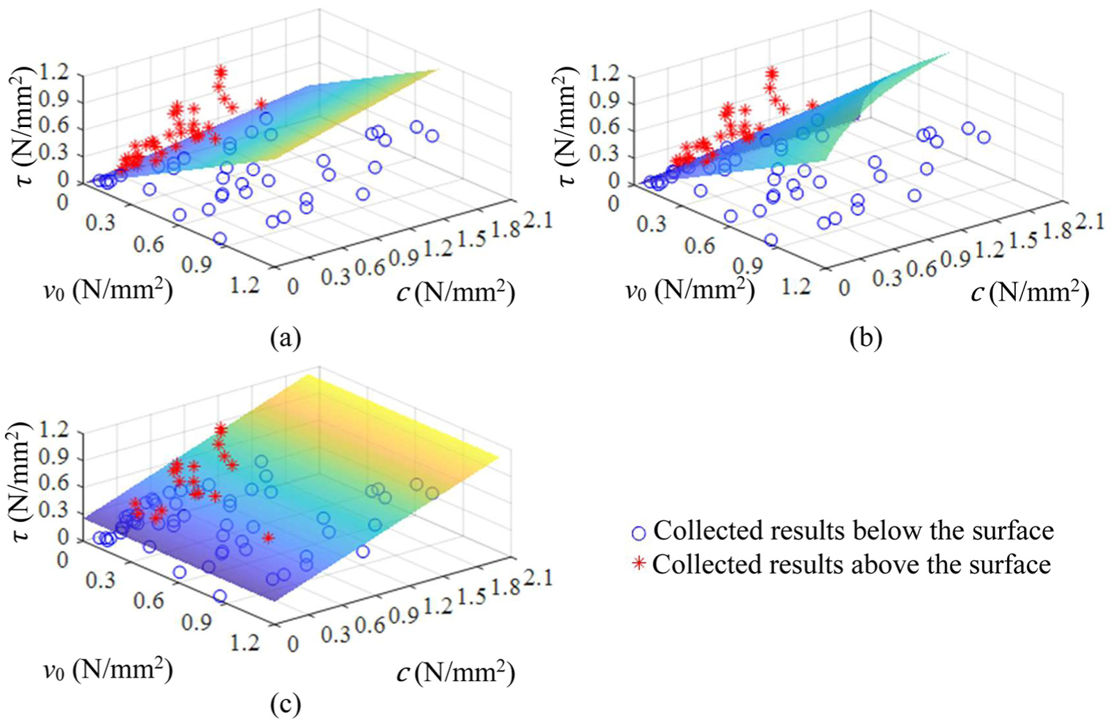
Surface of the prior mean function: (a) Model 1, (b) Model 2, and (c) Model 3.

To effectively train the prior GP models, the number of set of experimental results should be 10 times or more of that of the calibration parameters (Higdon et al., 2008). There are two calibration parameters in our prior GP models, and it needs 20 sets of experimental results at least. We used the 78 sets of experimental results in Appendix 1.

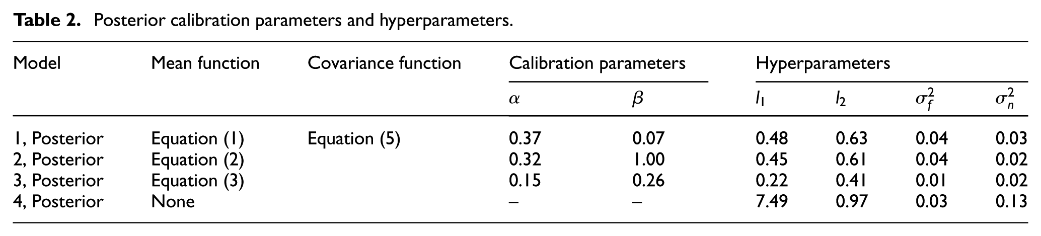
We established the log likelihood following equation (6) and then maximized the log likelihood using the conjugate gradient method (Rasmussen and Williams, 2006). There was no divergence issue or heavy time burden in the procedure. The resultant posterior parameters are listed in Table 2. They determine the posterior GP models.

Table 2.

Posterior calibration parameters and hyperparameters.

Model	Mean function	Covariance function	Calibration parameters		Hyperparameters
Model	Mean function	Covariance function	α	β	$l_{1}$	$l_{2}$	$σ_{f}^{2}$	$σ_{n}^{2}$
1, Posterior	Equation (1)	Equation (5)	0.37	0.07	0.48	0.63	0.04	0.03
2, Posterior	Equation (2)		0.32	1.00	0.45	0.61	0.04	0.02
3, Posterior	Equation (3)		0.15	0.26	0.22	0.41	0.01	0.02
4, Posterior	None		–	–	7.49	0.97	0.03	0.13

Interpolation based on the posterior GP models

We illustrate the posterior GP models in Figure 2. The posteriors GP models correct the bias of the prior models using the collected experimental results: the posterior mean functions of model 1 and model 3 become nonlinear, although their priors are linear. Through the correction, all the posterior mean functions show the nominal shear strength decreases with the increase of nominal compressive stress when such stress is high. The decrease is reasonable but the prior mean functions have not pointed out. In the posterior models, the decrease is due to the importance given to the covariance matrix, which is determined by the collected experimental results. It can be seen that the experimental results contribute significant information to correct the prior models without mechanical analysis.

Figure 2.

Surface of the posterior mean function: (a) Model 1, (b) Model 2, (c) Model 3, and (d) Model 4.

Reciprocally, the posteriors GP models relieve the uncertainty of the scattered experimental results using the prior mean functions, which represent engineering judgments. After relieving the uncertainty, the posterior GP models reveal latent relationships between the inputs and the outputs, and quantitatively specify the remaining uncertainty of the latent relationships.

We use two statistical indicators to evaluate the posterior GP models: the standardized mean squared error (SMSE) to the experimental results, and the standard deviation $σ$ combining $σ_{f}$ and $σ_{n}$ . The former represents how well the GP models interpolate in terms of agreement with the experimental results, and the latter represents how certain the GP models are about their interpolation. A favorable model has small SMSE and σ, indicating it is comparatively unbiased and certain. We list the two indicators of the posterior GP models in Table 3.

Table 3.

Statistical indicators of the posterior GP models.

Model	Standardized mean squared error (SMSE)	Standard deviation σ
1, Posterior	0.50	0.27
2, Posterior	0.49	0.24
3, Posterior	0.47	0.17
4, Posterior	0.54	0.40

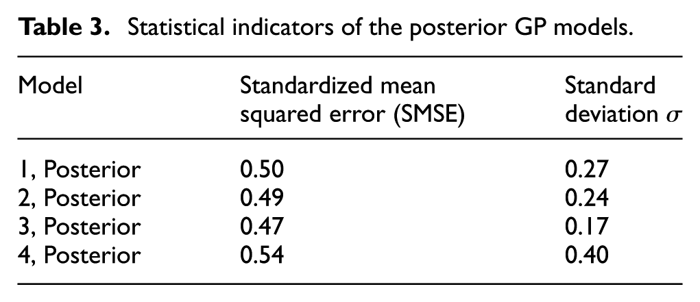
Table 3 indicates that the posterior GP model 3 is more favorable than other models. However, it excludes the influences of the cohesion $v_{0}$ and then potentially be less flexible. Therefore, we kept both the GP model 1 and 3 and then verified their interpolation and prediction.

The SMSEs in Table 3 are not small because we have used simple—or parsimonious—prior models. The parsimony is favorable and it can ensure the stability of prediction in terms of Bayesian inference. We can reduce the SMSEs using complicated prior models. However, the complicated models could introduce more calibration parameters that are difficult to measure, and then the training data would become inadequate. As an alternative, we can reduce the SESEs by optimizing the posterior GP models (Hastie et al., 2001; Nocedal and Wright, 2006). The optimization is meaningful for interpolation problems in which we have known all the experimental results. We illustrate the optimized GP model 1 and model 3 in Figure 3 and compare their interpolation with the experimental results in Figure 4. Figures 3 and 4 show that the optimized models are in good agreement with the known experimental results. Because the experimental results are heavily scattered, the agreement is very difficult to achieve using deterministic regression.

Figure 3.

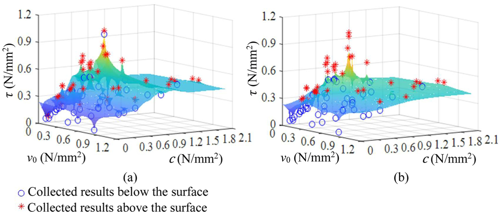
Surface of the optimized mean function: (a) Model 1 and (b) Model 3.

Figure 4.

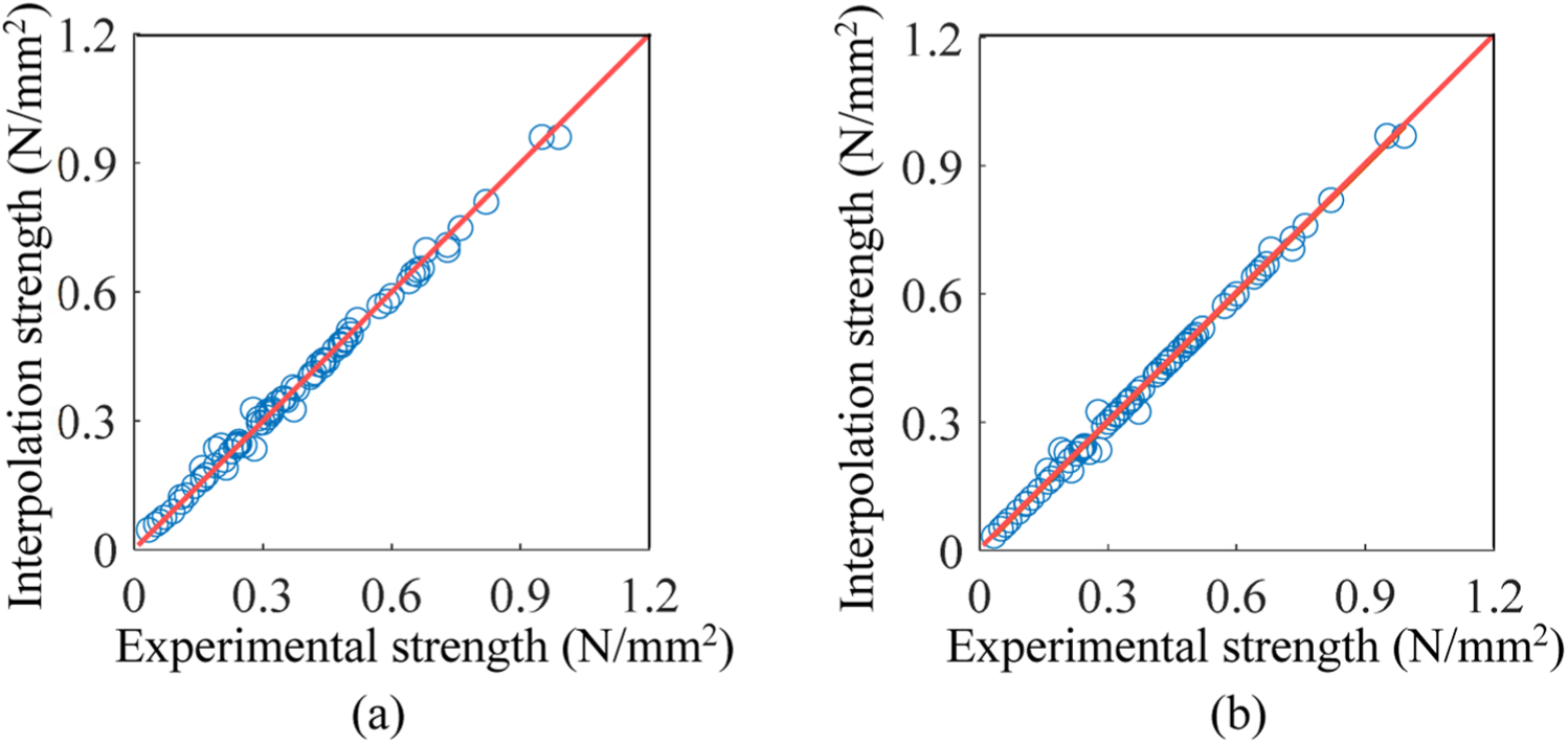
Interpolation results of the optimized GP models: (a) Model 1 and (b) Model 3.

Predication based on the updated GP models

In this section, we use the posterior GP model 1 and model 3 to predict new experimental results, which are from our own experiments and have not been used in model training. We constructed six 240-mm-thick fire-clay brick URM walls following the Chinese Code for Design of Masonry Structures (GB50003-2011, 2011) and determined their shear resistance through pseudo-static experiments. The experimental setup and the loading procedure are illustrated in Figure 5, and the experimental parameters and results are listed in Table 4. Other details of the experiments can be found elsewhere (Peng et al., 2016). Together with other parameters, Table 4 lists the aspect ratio of the specimens. This parameter influences the failure mode and shear resistance, but it is not considered in the prior GP models. We will show that the GP models suffer from missing the parameter.

Figure 5.

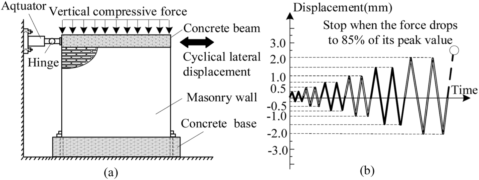
Pseudo-static experimental setup and lateral loading procedure: (a) experimental setup and (b) lateral loading procedure.

Table 4.

Experimental parameters and results.

Wall no.	Cohesion of masonry $v_{0}$ (N/mm²)	Nominal compressive stress c (N/mm²)	Nominal shear strength τ (N/mm²)	Parameters not considered in the prior GP models
Wall no.	Cohesion of masonry $v_{0}$ (N/mm²)	Nominal compressive stress c (N/mm²)	Nominal shear strength τ (N/mm²)	Aspect ratio of the wall	Area ratio of opening	Aspect ratio of the solid part of the wall
W1	0.26	0.43	0.74	0.75	0	0.75
W2	0.34	0.54	0.86	0.75	0	0.75
W3	0.34	0.55	0.66	0.75	0.11	0.38
W4	0.36	0.54	0.67	0.75	0.16	0.56
W5	0.36	0.52	0.72	1.25	0	1.25
W6	0.25	0.42	0.34	1.25	0.11	0.65

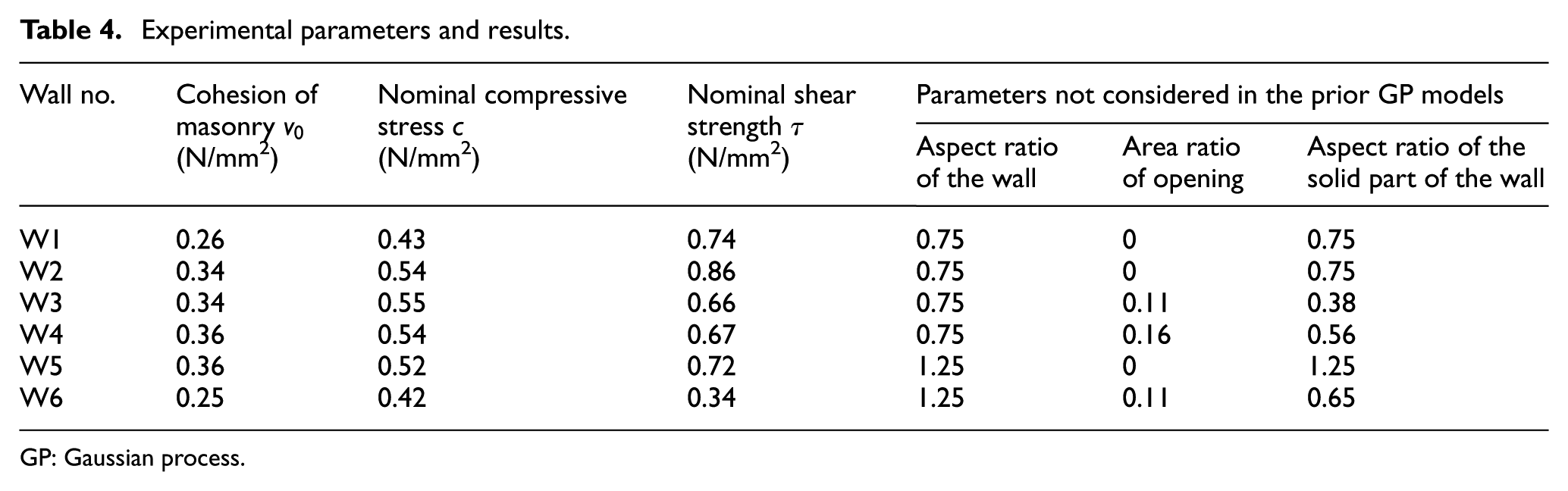
GP: Gaussian process.

For each set of $v_{0}$ and c in Table 4, we can predict a normal PDF for τ using the posterior GP model 1 and 3. Before each predication, we updated the posterior GP models using the other five sets of the experimental results. The predicted normal PDFs are specified in Table 5. In Table 5, the means are the estimators of τ, the standard deviations describe the remaining uncertainty of the estimators, and the SMSEs describe the global agreement between the estimators and the experimental results.

Table 5.

Predicted normal PDF of the nominal shear strength τ.

Wall no.	Experimental results (N/mm²)	Normal PDF predicted by updated GP model 1			Normal PDF predicted by updated GP model 3
Wall no.	Experimental results (N/mm²)	Mean $μ_{1}$ (N/mm²)	Standard deviation $σ_{1}$ (N/mm²)	SMSE	Mean $μ_{3}$ (N/mm²)	Standard deviation $σ_{3}$ (N/mm²)	SMSE
W1	0.74	0.45	0.25	0.47	0.45	0.20	0.19
W2	0.86	0.52	0.25	0.48	0.56	0.20	0.20
W3	0.66	0.54	0.25	0.48	0.63	0.20	0.20
W4	0.67	0.53	0.25	0.48	0.64	0.20	0.20
W5	0.72	0.52	0.25	0.48	0.61	0.20	0.20
W6	0.34	0.47	0.25	0.46	0.47	0.20	0.19

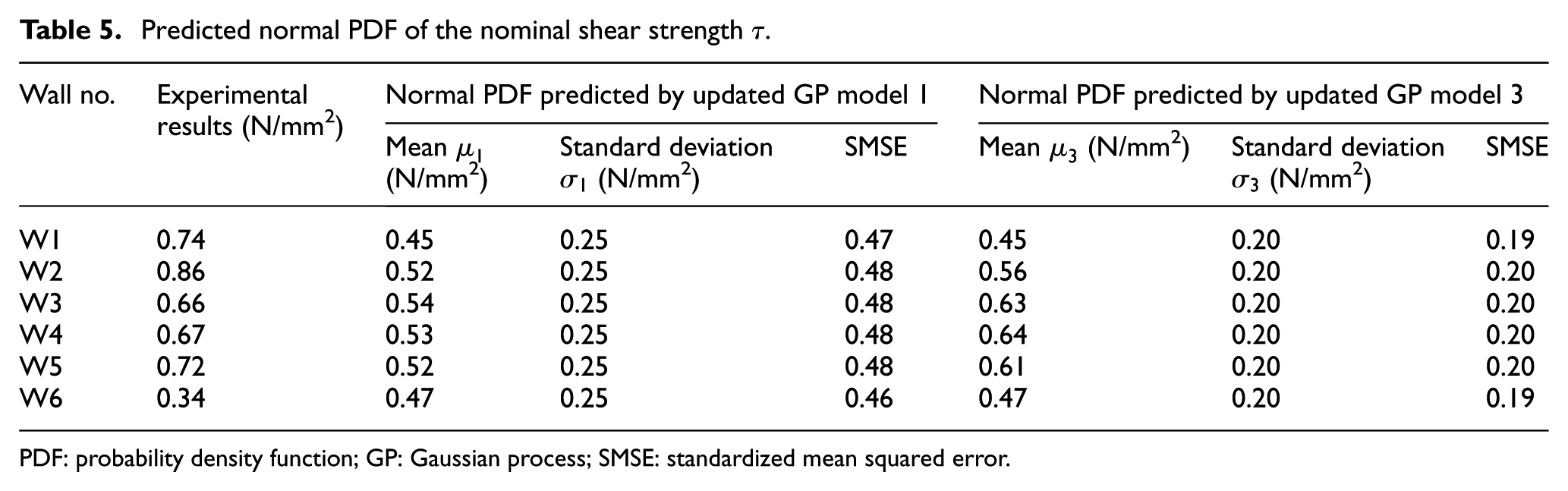
PDF: probability density function; GP: Gaussian process; SMSE: standardized mean squared error.

The GP models give information that is unavailable if using deterministic models. The SMSEs indicate that the estimators given by the updated GP model 3 are in better agreement with experimental results, and the stand deviations indicate that the estimators given by the updated GP model 3 are more certain. The updated GP models still have uncertainty, as any deterministic models do; but they can quantitatively specify their uncertainty, unlike the deterministic models that fail to do so. With this feature, the GP models can give clear information for decision-making in real-world practices.

The updated GP model 3 predicts well for the walls having aspect ratios below 0.6, like wall 3 and wall 4. Because the small aspect ratio makes the two walls more likely to fail in diagonal shear mode, which is in accordance with the judgment of the prior GP model 3. The same model predicts poor for the other walls that have aspect ratios above 0.6, because the big aspect ratio makes the walls less likely to fail in diagonal shear modes. For such walls, the prior GP model 3 is significantly biased and then the posterior model cannot predict well.

The COV of all experimental results is 0.26, while the COV of all estimators given by the updated GP model 3 is 0.15. The small COV denotes the mean function of the updated GP model 3 is smooth (or stable) enough, and thus, the model is favorable for predication. The smooth mean function indicates that the training and updating procedures have penalized the unnecessary complexity of the model, as has explained for equation (6).

The GP models have other potential advantages for real-world practices. First, they are efficient because they do not involve the constitutive relationships and the failure criteria of the URM. Using the GP models, we can directly predict the shear resistance without conducting a full range of iterative analysis. Second, they specify the normal PDFs of the nominal shear resistance. The normal PDFs give adequate information for decision-making and facilitate the reliability index calculation by simplifying the performance functions. Third, the GP models are easily improvable. Their updating runs completely on the new experimental results as those listed in Table 4, while involving no operation on the previously used results as those listed in Appendix 1. The updating can be triggered again whenever other experimental results arrive.

With the above-mentioned features, the GP models can predict the shear resistance using simple prior models and a few parameters that can be easily measured. Their prediction can be efficiently improved along with the accumulation of experimental results.

Conclusion

Uncertainty is a major issue in the shear resistance estimation for URM walls. To account for the uncertainty, we converted the deterministic shear resistance models to prior GP models, trained the prior GP models into posterior ones using the experimental results collected from literature, and then verified the performance of the GP models in interpolation and predication. The following conclusions are drawn from this research.

The GP models can combine and weight the engineering judgments and the information from experimental results. They use the engineering judgments to compensate for information inadequateness of the scattered experimental results. Meanwhile, they use the information from the experimental results to relieve the potential bias of the engineering judgments. Therefore, they can realize interpolations that are in good agreement with heavily scattered experimental results.

The GP models account for both parameter uncertainty and model uncertainty. They allow us to estimate the shear resistance of the URM walls, even when we are not sure about the parameters and the failure mechanisms. They are flexible and compatible with a wide range of simple prior models. Meanwhile, their training or updating procedures automatically penalize the unnecessary complexity and then result in stable posterior mean functions that are favorable for estimation.

The GP models can determine normal PDFs for the shear resistance. The normal PDFs can generate shear resistance estimators and then quantitatively specify the estimators’ remaining uncertainty. Having the PDFs, we can determine whether we should modify the priors to relieve the bias, or whether we should use more experimental results to further update the posterior GP models. The normal PDFs also facilitate reliability index calculations in structural assessments. With these advantages, the GP models are potentially useful in the shear resistance estimation for the URM walls.

Footnotes

Appendix 1

Table 6.

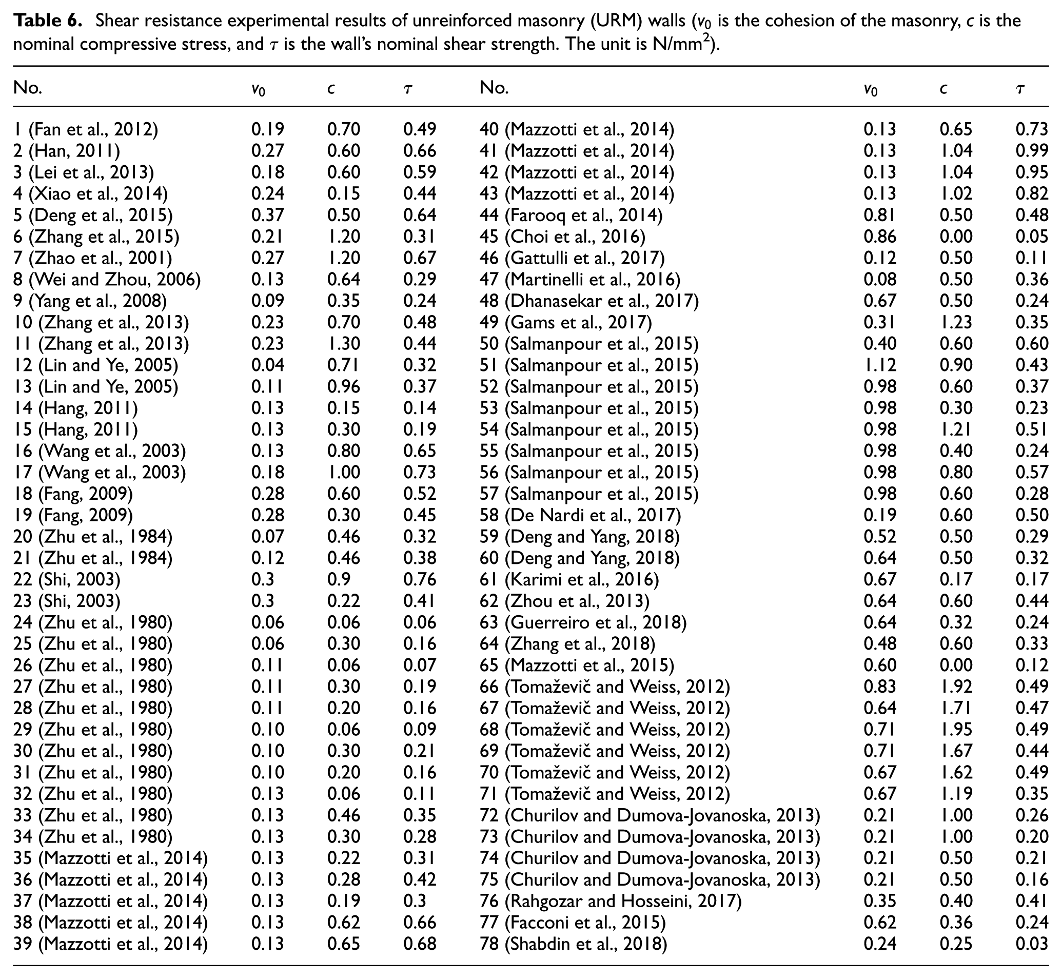
Shear resistance experimental results of unreinforced masonry (URM) walls ( $v_{0}$ is the cohesion of the masonry, c is the nominal compressive stress, and τ is the wall’s nominal shear strength. The unit is N/mm²).

No.	$v_{0}$	c	τ	No.	$v_{0}$	c	τ
1 (Fan et al., 2012)	0.19	0.70	0.49	40 (Mazzotti et al., 2014)	0.13	0.65	0.73
2 (Han, 2011)	0.27	0.60	0.66	41 (Mazzotti et al., 2014)	0.13	1.04	0.99
3 (Lei et al., 2013)	0.18	0.60	0.59	42 (Mazzotti et al., 2014)	0.13	1.04	0.95
4 (Xiao et al., 2014)	0.24	0.15	0.44	43 (Mazzotti et al., 2014)	0.13	1.02	0.82
5 (Deng et al., 2015)	0.37	0.50	0.64	44 (Farooq et al., 2014)	0.81	0.50	0.48
6 (Zhang et al., 2015)	0.21	1.20	0.31	45 (Choi et al., 2016)	0.86	0.00	0.05
7 (Zhao et al., 2001)	0.27	1.20	0.67	46 (Gattulli et al., 2017)	0.12	0.50	0.11
8 (Wei and Zhou, 2006)	0.13	0.64	0.29	47 (Martinelli et al., 2016)	0.08	0.50	0.36
9 (Yang et al., 2008)	0.09	0.35	0.24	48 (Dhanasekar et al., 2017)	0.67	0.50	0.24
10 (Zhang et al., 2013)	0.23	0.70	0.48	49 (Gams et al., 2017)	0.31	1.23	0.35
11 (Zhang et al., 2013)	0.23	1.30	0.44	50 (Salmanpour et al., 2015)	0.40	0.60	0.60
12 (Lin and Ye, 2005)	0.04	0.71	0.32	51 (Salmanpour et al., 2015)	1.12	0.90	0.43
13 (Lin and Ye, 2005)	0.11	0.96	0.37	52 (Salmanpour et al., 2015)	0.98	0.60	0.37
14 (Hang, 2011)	0.13	0.15	0.14	53 (Salmanpour et al., 2015)	0.98	0.30	0.23
15 (Hang, 2011)	0.13	0.30	0.19	54 (Salmanpour et al., 2015)	0.98	1.21	0.51
16 (Wang et al., 2003)	0.13	0.80	0.65	55 (Salmanpour et al., 2015)	0.98	0.40	0.24
17 (Wang et al., 2003)	0.18	1.00	0.73	56 (Salmanpour et al., 2015)	0.98	0.80	0.57
18 (Fang, 2009)	0.28	0.60	0.52	57 (Salmanpour et al., 2015)	0.98	0.60	0.28
19 (Fang, 2009)	0.28	0.30	0.45	58 (De Nardi et al., 2017)	0.19	0.60	0.50
20 (Zhu et al., 1984)	0.07	0.46	0.32	59 (Deng and Yang, 2018)	0.52	0.50	0.29
21 (Zhu et al., 1984)	0.12	0.46	0.38	60 (Deng and Yang, 2018)	0.64	0.50	0.32
22 (Shi, 2003)	0.3	0.9	0.76	61 (Karimi et al., 2016)	0.67	0.17	0.17
23 (Shi, 2003)	0.3	0.22	0.41	62 (Zhou et al., 2013)	0.64	0.60	0.44
24 (Zhu et al., 1980)	0.06	0.06	0.06	63 (Guerreiro et al., 2018)	0.64	0.32	0.24
25 (Zhu et al., 1980)	0.06	0.30	0.16	64 (Zhang et al., 2018)	0.48	0.60	0.33
26 (Zhu et al., 1980)	0.11	0.06	0.07	65 (Mazzotti et al., 2015)	0.60	0.00	0.12
27 (Zhu et al., 1980)	0.11	0.30	0.19	66 (Tomaževič and Weiss, 2012)	0.83	1.92	0.49
28 (Zhu et al., 1980)	0.11	0.20	0.16	67 (Tomaževič and Weiss, 2012)	0.64	1.71	0.47
29 (Zhu et al., 1980)	0.10	0.06	0.09	68 (Tomaževič and Weiss, 2012)	0.71	1.95	0.49
30 (Zhu et al., 1980)	0.10	0.30	0.21	69 (Tomaževič and Weiss, 2012)	0.71	1.67	0.44
31 (Zhu et al., 1980)	0.10	0.20	0.16	70 (Tomaževič and Weiss, 2012)	0.67	1.62	0.49
32 (Zhu et al., 1980)	0.13	0.06	0.11	71 (Tomaževič and Weiss, 2012)	0.67	1.19	0.35
33 (Zhu et al., 1980)	0.13	0.46	0.35	72 (Churilov and Dumova-Jovanoska, 2013)	0.21	1.00	0.26
34 (Zhu et al., 1980)	0.13	0.30	0.28	73 (Churilov and Dumova-Jovanoska, 2013)	0.21	1.00	0.20
35 (Mazzotti et al., 2014)	0.13	0.22	0.31	74 (Churilov and Dumova-Jovanoska, 2013)	0.21	0.50	0.21
36 (Mazzotti et al., 2014)	0.13	0.28	0.42	75 (Churilov and Dumova-Jovanoska, 2013)	0.21	0.50	0.16
37 (Mazzotti et al., 2014)	0.13	0.19	0.3	76 (Rahgozar and Hosseini, 2017)	0.35	0.40	0.41
38 (Mazzotti et al., 2014)	0.13	0.62	0.66	77 (Facconi et al., 2015)	0.62	0.36	0.24
39 (Mazzotti et al., 2014)	0.13	0.65	0.68	78 (Shabdin et al., 2018)	0.24	0.25	0.03

Declaration of Conflicting Interests

The author(s) declared no potential conflicts of interest with respect to the research, authorship, and/or publication of this article.

Funding

The author(s) disclosed receipt of the following financial support for the research, authorship, and/or publication of this article: The research is financially supported by the National Natural Science Foundation of China under Grant No. 51208300.

ORCID iD

Bin Peng

References

ACI 530-05 (2005) Building Code Requirements for Masonry Structures. Farmington Hills, MI: American Concrete Institute.

Ali

Page

(1989) Finite element model for masonry subjected to concentrated loads. Journal of Structural Engineering 114(8): 1761–1784.

Ang

AH-S

Tang

(1975) Probability Concepts in Engineering Planning and Design (Basic Principles), vol. 1. New York: John Wiley & Sons.

Atamturktur

Hemez

Laman

(2012) Uncertainty quantification in model verification and validation as applied to large scale historic masonry monuments. Engineering Structures 43: 221–234.

Binda

Pina-Henriques

Anzani

et al . (2006) A contribution for the understanding of load-transfer mechanisms in multi-leaf masonry walls: Testing and modelling. Engineering Structures 28: 1132–1148.

Bolhassani

Hamid

Johnson

et al . (2016) Shear strength expression for partially grouted masonry walls. Engineering Structures 127: 475–494.

Bruggi

Milani

(2015) Optimal FRP reinforcement of masonry walls out-of-plane loaded: a combined homogenization–topology optimization approach complying with masonry strength domain. Computers & Structures 153: 49–74.

Brunner

Shing

(1996) Shear strength of reinforced masonry walls. The Masonry Society Journal 14(1): 65–77.

Calderón

Sandoval

Arnau

(2017) Shear response of partially-grouted reinforced masonry walls with a central opening: testing and detailed micro-modelling. Materials & Design 118: 122–137.

10.

Casolo

(2004) Modelling in-plane micro-structure of masonry walls by rigid elements. International Journal of Solids and Structures 41(13): 3625–3641.

11.

Choi

Bae

Choi

(2016) Lateral resistance of unreinforced masonry walls strengthened with engineered cementitious composite. International Journal of Civil Engineering 14(6): 411–424.

12.

Churilov

Dumova-Jovanoska

(2013) In-plane shear behaviour of unreinforced and jacketed brick masonry walls. Soil Dynamics and Earthquake Engineering 50: 85–105.

13.

Clementi

Gazzani

Poiani

et al . (2016) Assessment of seismic behaviour of heritage masonry buildings using numerical modelling. Journal of Building Engineering 8: 29–47.

14.

Colonna

Imperatore

Zucconi

et al . (2017) Post-seismic damage assessment of a historical masonry building: the case study of a school in Teramo. Key Engineering Materials 747: 620–627.

15.

Como

(2014) Seismic strength of reinforced multi-storey masonry walls. Key Engineering Materials 624: 19–26.

16.

Costa

Penna

Arêde

et al . (2015) Simulation of masonry out-of-plane failure modes by multi-body dynamics. Earthquake Engineering & Structural Dynamics 44(14): 2529–2549.

17.

D’Ayala

Shi

(2011) Modeling masonry historic buildings by multi-body dynamics. International Journal of Architectural Heritage 5(4–5): 483–512.

18.

De Nardi

Cecchi

Ferrara

(2017) The influence of self-healing capacity of lime mortars on the behaviour of brick-mortar masonry subassemblies. Key Engineering Materials 747: 465–471.

19.

Deng

Yang

(2018) Cyclic testing of unreinforced masonry walls retrofitted with engineered cementitious composites. Construction and Building Materials 177: 395–408.

20.

Deng

Fan

Gao

et al . (2015) Experimental investigation on seismic behavior of damaged brick masonry wall strengthened with ECC splint. Engineering Mechanics 32(4): 120–129 (in Chinese).

21.

Dhanasekar

Kleeman

Page

(1985) Biaxial stress-strain relations for brick masonry. Journal of Structural Engineering 111(5): 1085–1100.

22.

Dhanasekar

Thamboo

Nazir

(2017) On the in-plane shear response of the high bond strength concrete masonry walls. Materials and Structures 50(5): 214.

23.

Dymiotis

Gutlederer

(2002) Allowing for uncertainties in the modelling of masonry compressive strength. Construction and Building Materials 16(8): 443–452.

24.

Ellingwood

(1981) Analysis of reliability for masonry structures. Journal of the Structural Division 107(5): 757–773.

25.

EN 1996/Eurocode 6 (2005) Design of Masonry Structures. Brussels: European Committee for Standardization (CEN).

26.

Facconi

Conforti

Minelli

et al . (2015) Improving shear strength of unreinforced masonry walls by nano-reinforced fibrous mortar coating. Materials and Structures 48(8): 2557–2574.

27.

Fan

Zuo

Guo

(2012) Experimental study on the test of masonry walls strengthened with CFRP under low-cyclic loads. Journal of Shenyang Jianzhu University 28(2): 208–214 (in Chinese).

28.

Fang

(2009) Experimental research on seismic shear strength and seismic behavior of autoclaved fly ash brick wall. PhD Thesis, Changsha University of Science & Technology, Changsha, China (in Chinese).

29.

Farooq

Shahid

Ilyas

(2014) Seismic performance of masonry strengthened with steel strips. KSCE Journal of Civil Engineering 18(7): 2170–2180.

30.

Gams

Tomaževič

Berset

(2017) Seismic strengthening of brick masonry by composite coatings: an experimental study. Bulletin of Earthquake Engineering 15(10): 4269–4298.

31.

Gattulli

Lofrano

Paolone

et al . (2017) Performances of FRP reinforcements on masonry buildings evaluated by fragility curves. Computers & Structures 190: 150–161.

32.

GB50003-2011 (2011) Code for Design of Masonry Structures. Beijing, China (in Chinese): China Architecture and Building Press.

33.

Gentilini

Franzoni

Graziani

et al . (2015) Mechanical properties of fired-clay brick masonry models in moist and dry conditions. Key Engineering Materials 624: 307–312.

34.

Grimm

(1988) Brick masonry workmanship statistics. Journal of Construction Engineering and Management 114(1): 147–149.

35.

Guerreiro

Proença

Ferreira

et al . (2018) Experimental characterization of in-plane behaviour of old masonry walls strengthened through the addition of CFRP reinforced render. Composites Part B: Engineering 148: 14–26.

36.

Haach

Vasconcelos

Lourenço

(2013) Proposal of a design model for masonry walls subjected to in-plane loading. Journal of Structural Engineering 139(4): 537–547.

37.

Han

(2011) Research on vertical loading control and specimen design for seismic experiments of masonry shear walls. PhD Thesis, Taiyuan University of Technology, Taiyuan, China (in Chinese).

38.

Hang

(2011) Comparison between simulation and experimental results of compressive and seismic resistance of masonry structures. PhD Thesis, Hunan University, Changsha, China (in Chinese).

39.

Hastie

Friedman

Tibshirani

(2001) The Elements of Statistical Learning. New York: Springer.

40.

Haukaas

Asce

Gardoni

(2011) Model uncertainty in finite-element analysis: Bayesian finite elements. Journal of Engineering Mechanics 137(8): 519–526.

41.

Hendry

(1982) Safety factors in limit states design of masonry. International Journal of Masonry Construction 2(4): 178–181.

42.

Higdon

Gattiker

Williams

et al . (2008) Computer model calibration using high-dimensional output. Journal of the American Statistical Association 103(482): 570–583.

43.

Hoff

(2009) A First Course in Bayesian Statistical Methods. New York: Springer.

44.

Janaraj

Dhanasekar

(2014) Finite element analysis of the in-plane shear behaviour of masonry panels confined with reinforced grouted cores. Construction and Building Materials 65: 495–506.

45.

Kalliontzis

Schultz

(2017) Improved estimation of the reverse-cyclic behavior of fully-grouted masonry shear walls with unbonded post-tensioning. Engineering Structures 145: 83–96.

46.

Karimi

Kheyroddin

et al . (2016) Experimental and numerical study on seismic behavior of an infilled masonry wall compared to an arched masonry wall. Structures 8: 144–153.

47.

Köksal

Jafarov

Doran

et al . (2013) Computational material modeling of masonry walls strengthened with fiber reinforced polymers. Structural Engineering and Mechanics 48: 737–755.

48.

Konthesingha

KMC

Masia

Petersen

et al . (2013) Static cyclic in-plane shear response of damaged masonry walls retrofitted with NSM FRP strips—an experimental evaluation. Engineering Structures 50: 126–136.

49.

Lei

Zhou

Wang

(2013) Seismic behavior of reinforced masonry brick wall with basalt fiber reinforced material. Journal of South China University of Technology (3): 43–49,75 (in Chinese).

50.

Lemos

(2007) Discrete element modeling of masonry structures. International Journal of Architectural Heritage 1(2): 190–213.

51.

Lin

(2005) Experimental investigation on masonry wall strengthened with FRP. Building Structure 35(3): 21–27 (in Chinese).

52.

Lourenço

(1996) Computational strategies for masonry structures. PhD Thesis, Delft University of Technology, Delft.

53.

Lourenço

(2010) Recent advances in masonry modelling: micromodelling and homogenization. In: Galvanetto

Aliabadi

MHF

(eds) Multiscale Modeling in Solid Mechanics: Computational Approaches. London: World Scientific Publishing, pp. 251–294.

54.

Lourenço

Milani

Tralli

(2007) Analysis of masonry structures: review of and recent trends of homogenization techniques. Canadian Journal of Civil Engineering 34: 1443–1457.

55.

Hao

(2001) Homogenization of masonry using numerical simulations. Journal of Engineering Mechanics 127(5): 421–431.

56.

Martinelli

Perri

Sguazzo

et al . (2016) Cyclic shear-compression tests on masonry walls strengthened with alternative configurations of CFRP strips. Bulletin of Earthquake Engineering 14(6): 1695–1720.

57.

Mazzotti

Ferracuti

Bellini

(2015) Experimental bond tests on masonry panels strengthened by FRP. Composites Part B: Engineering 80: 223–237.

58.

Mazzotti

Sassoni

Pagliai

(2014) Determination of shear strength of historic masonries by moderately destructive testing of masonry cores. Construction and Building Materials 54: 421–431.

59.

Mojsilović

Stewart

(2015) Probability and structural reliability assessment of mortar joint thickness in load-bearing masonry walls. Structural Safety 52: 209–218.

60.

Mojsilović

Simundic

Page

(2010) Masonry wallettes with damp-proof course membrane subjected to cyclic shear: an experimental study. Construction and Building Materials 24(11): 2135–2144.

61.

Nazar

Sinha

(2007a) Fatigue behaviour of interlocking grouted stabilised mud-fly ash brick masonry. International Journal of Fatigue 29(5): 953–961.

62.

Nazar

Sinha

(2007b) Loading-unloading curves of interlocking grouted stabilised sand-flyash brick masonry. Materials and Structures 40(7): 667–678.

63.

Neal

(1996) Bayesian Learning for Neural Networks (Lecture Notes in Statistics). New York: Springer. Available at: http://link.springer.com/10.1007/978-1-4612-0745-0

64.

Nocedal

Wright

(2006) Numerical Optimization. 2nd ed.New York: Springer.

65.

Noor-E-Khuda

Dhanasekar

(2018) Masonry walls under combined in-plane and out-of-plane loadings. Journal of Structural Engineering 144(2): 1–10.

66.

Orduña

Lourenço

(2003) Cap model for limit analysis and strengthening of masonry structures. Journal of Structural Engineering 129(10): 1367–1375.

67.

Page

Samarasinghe

Hendry

(1980) The failure of masonry shear walls. International Journal of Masonry Construction 1(2): 52–57.

68.

Peng

Wang

Zong

et al . (2018) Homogenization strategy for brick masonry walls under in-plane loading. Construction and Building Materials 163: 656–667.

69.

Peng

Wang

et al . (2016) Pseudo-static tests on the seismic performances of masonry walls. Journal of University of Shanghai for Science and Technology 38(4): 402–408 (in Chinese).

70.

Peralta

Mosalam

(2016) Multiscale homogenization analysis of the effective elastic properties of masonry structures. Journal of Materials in Civil Engineering 28(8): 04016056.

71.

Rahgozar

Hosseini

(2017) Experimental and numerical assessment of in-plane monotonic response of ancient mortar brick masonry. Construction and Building Materials 155: 892–909.

72.

Rasmussen

Williams

CKI

(2006) Gaussian Processes for Machine Learning. Cambridge, MA: The MIT Press.

73.

Roca

Cervera

Gariup

et al . (2010) Structural analysis of masonry historical constructions. Classical and advanced approaches. Archives of Computational Methods in Engineering 17(3): 299–325.

74.

Rota

Penna

Magenes

(2014) A framework for the seismic assessment of existing masonry buildings accounting for different sources of uncertainty. Earthquake Engineering & Structural Dynamics 43(7): 1045–1066.

75.

Salmanpour

Mojsilović

Schwartz

(2015) Displacement capacity of contemporary unreinforced masonry walls: an experimental study. Engineering Structures 89: 1–16.

76.

Schultz

Hutchinson

Cheok

(1998) Seismic performance of masonry walls with bed joint reinforcement. In: Srivastava

Fenves

Domer

Ang

AHS

(eds) Structural Engineers World Congress. San Francisco, CA.

77.

Shabdin

Attari

NKA

Zargaran

(2018) Experimental study on seismic behavior of Un-Reinforced Masonry (URM) brick walls strengthened with shotcrete. Bulletin of Earthquake Engineering 16: 3931–3956.

78.

Shi

(2003) Theory and Design of Masonry Structures. 2nd ed.Beijing, China: China Architecture & Building Press (in Chinese).

79.

Shing

Schuller

Hoskere

(1990) In-plane resistance of reinforced masonry shear walls. Journal of Structural Engineering 116(3): 619–640.

80.

Snozzi

Molinari

J-F

(2013) A cohesive element model for mixed mode loading with frictional contact capability. International Journal for Numerical Methods in Engineering 93(5): 510–526.

81.

Soize

(2013) Stochastic modeling of uncertainties in computational structural dynamics-recent theoretical advances. Journal of Sound and Vibration 332(10): 2379–2395.

82.

Sui

(2007) Improving the prediction of the behaviour of masonry wall panels using model updating and artificial intelligence techniques. PhD Thesis, University of Plymouth, Plymouth, Devon.

83.

Sutcliffe

Page

(2001) Lower bound limit analysis of unreinforced masonry shear walls. Computers & Structures 79: 1295–1312.

84.

Theodossopoulos

Sinha

(2013) A review of analytical methods in the current design processes and assessment of performance of masonry structures. Construction and Building Materials 41: 990–1001.

85.

Tomaževič

(2009) Shear resistance of masonry walls and Eurocode 6: shear versus tensile strength of masonry. Materials and Structures 42(7): 889–907.

86.

Tomaževič

Weiss

(2010) Displacement capacity of masonry buildings as a basis for the assessment of behavior factor: an experimental study. Bulletin of Earthquake Engineering 8(6): 1267–1294.

87.

Tomaževič

Weiss

(2012) Robustness as a criterion for use of hollow clay masonry units in seismic zones: an attempt to propose the measure. Materials and Structures 45(4): 541–559.

88.

Tomaževič

Lutman

Petković

(1996) Seismic behavior of masonry walls: experimental simulation. Journal of Structural Engineering 122(9): 1040–1047.

89.

Torres

Almazán

Sandoval

et al . (2017) Operational modal analysis and FE model updating of the metropolitan cathedral of Santiago, Chile. Engineering Structures 143: 169–188.

90.

Vasconcelos

Lourenço

(2009) Experimental characterization of stone masonry in shear and compression. Construction and Building Materials 23(11): 3337–3345.

91.

Wang

(2003) An investigation of the aseismatic behavior of masonry structures strengthened by carbon fiber reinforced plastics. Industrial Construction 33(9): 11–13 (in Chinese).

92.

Wei

Zhou

(2006) Experimental study on masonry walls strengthened with CFRP. Engineering Mechanics 23(S2): 150–154 (in Chinese).

93.

Xiao

Zhang

et al . (2014) Experimental study on shear capacity of short-leg masonry shear wall reinforced with concrete splint. Earthquake Resistant Engineering and Retrofitting 36(1): 48–51, 47 (in Chinese).

94.

Yang

Wang

et al . (2008) Experimental study on strengthening brick walls of low strength with high strength steel wire and polymer mortar. Journal of Disaster Prevent and Mitigation Engineering (4): 473–478 (in Chinese).

95.

Zhang

Shi

(2013) Experimental study on seismic behavior of brick walls strengthened with embedded bars. Journal of Building Structures 34(5): 145–150 (in Chinese).

96.

Zhang

et al . (2018) Experimental study on seismic performance of fire-exposed perforated brick masonry wall. Construction and Building Materials 180: 77–91.

97.

Zhang

Yang

et al . (2015) Finite element modelling of FRP-reinforced masonry walls under in-plane loadings. Engineering Mechanics 32(12): 233–242 (in Chinese).

98.

Zhao

Zhang

Xie

et al . (2001) Experimental study on seismic reinforcement of brick masonry walls with continuous carbon fiber sheet. Earthquake Engineering and Engineering Vibration 21(2): 89–95 (in Chinese).

99.

Zhou

Lei

Wang

(2013) In-plane behavior of seismically damaged masonry walls repaired with external BFRP. Composite Structures 102: 9–19.

100.

Zhou

Zhu

Yang

et al . (2017) Shear capacity estimation of fully grouted reinforced concrete masonry walls using neural network and adaptive neuro-fuzzy inference system models. Construction and Building Materials 153: 937–947.

101.

Zhu

Jiang

(1980) Experimental study on basic performances of brick masonry under periodical loading. Journal of Tongji Univeristy (2): 1–14 (in Chinese).

102.

Zhu

Jiang

(1984) A study on aseismic capacity of brick wall strengthened with cement mortar reinforced with steel mesh. Earthquake Engineering and Engineering Dynamics 4(1): 69–83 (in Chinese).