Friction measurement and correction method in quasi-static tests of columns under combined axial and cyclic lateral loading

Abstract

In quasi-static tests of large-scale structural columns and/or columns under large axial loads, the lateral friction force between the column and the loading system can become a significant problem: they may cause considerable deviation between the measured lateral force and the actual reaction force of the column, especially under large axial compression load. Many researchers have come up with different methods to reduce or eliminate the influence of such friction force. In this article, previous treatments on the lateral friction force in quasi-static tests are first discussed. A shear force measurement device, for accurate measurement of the friction force, is then presented and calibrated. Based on the friction forces measured by the device in real tests, a simple model is proposed to predict the lateral friction force in quasi-static tests. Using the model, the measured lateral force in such tests can be corrected to obtain the actual reaction force of the column when a friction measurement device is absent. The proposed model and the correction method are then validated using results from several previous tests.

Keywords

friction correction friction measurement lateral friction quasi-static test structural columns

Introduction

In the field of seismic structural experiments of columns, quasi-static tests, which are also referred as low-cyclic reversed load tests, are the most prevalent test method. Most of the seismic experiments of columns were carried out using this testing method (Leon and Deierlein, 1996). Compared with pseudodynamic tests and shaking table tests, quasi-static tests are much more convenient and cost-effective, and much less labor-intensive. Hysteretic behavior, as well as seismic performance of the column, including loading capacity, ductility, energy dissipation capacity, and stiffness degradation behavior, can be obtained from the quasi-static test. Historical development and considerations for the quasi-static test method have also been discussed by Leon and Deierlein (1996).

In a typical setup of quasi-static test for columns, constant axial compression and cyclic lateral loading are applied to the column, which leads to friction forces at the sliding interface of the column and the axial loading device. For columns with a small section area and a small axial compression ratio, axial loading is usually small and the friction can be reduced and ignored using lubricants. However, with the development of servo-hydraulic technology, loading machines with a large load capacity of over 20,000 kN have been used in seismic structural experiments. Especially for some large-size columns and columns tested under a high axial compression ratio, the constant axial load applied can be very large. Lateral friction force has become a non-negligible problem and may cause considerable deviation on the measured hysteretic behavior of the column specimen. This effect has also been found and discussed by several studies (Feng et al., 2018; Hu, 2010; Jiang et al., 2014; Liu, 2016; Sun et al., 2017; Xiao et al., 2018; Zhang et al., 2015). Experimental results and the corresponding lateral friction forces from existing studies and measured in this article are listed in Table 1.

Table 1.

Influence of lateral friction force in quasi-static tests.

Sliding surfaces type	Axial force (kN)	Maximum lateral force (kN)	Lateral friction force (kN)	Proportion of friction force (%)	Friction coefficient ratio (%)
PTFE–steel (Liu, 2016)	1622	308	56.5	18.3	3.48
	2050	1746	20.6	1.2	1.00
	2310	1041	32.8	3.2	1.42
	4500	1202	24.3	2.0	0.54
	5300	343	139.3	40.6	2.63
	3700	602	94.1	15.6	2.54
	4150	3128	112.6	3.6	2.71
PTFE–steel (Feng et al., 2018)	6850	421.6	128.3	30.4	2.9
	6047	558.6	200.1	35.8	2.1
PTFE–steel (Sun et al., 2017)	200	79.0–92.4	6.0	6.5–7.6	3.0
Steel roller (Zhang et al., 2015)	2103	173	10.515	6.1	0.50
Steel roller (Hu, 2010)	1260	110	6.61	6.0	0.53

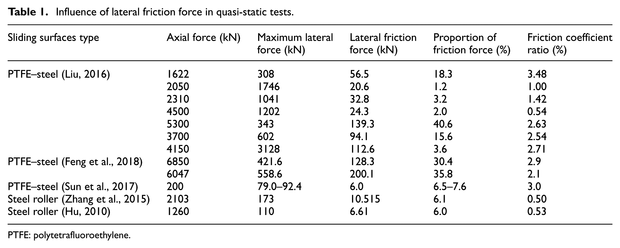
PTFE: polytetrafluoroethylene.

It is indicated that the lateral friction force can have a significant influence on the measurement of lateral force with respect to the actual reaction force, especially for specimens with a large axial compression force and a large cross-sectional area. Since the friction force tends to keep constant during the test, the lateral friction force can cause larger measurement deviation than those shown in Table 1 at the initial stage of loading when the overall lateral force is low. In this way, it is necessary to deduct the lateral friction force from the measured load to obtain the actually load resisted by the column specimen. However, it is indicated from Table 1 that the lateral friction force depends not only on the applied axial force but also on the friction interface configuration and experiment environment, which makes the lateral friction force more difficult to be characterized.

Many researchers have realized this problem and proposed different approaches to reduce or eliminate this influence, such as using some friction reduction treatment or new loading methods (Azizinamini et al., 1994; Fam et al., 2004; Guo and Lu, 2004; Lu and Lu, 2000; Naqvi and El-Salakawy, 2016; Saatcioglu and Ozcebe, 1989; Stephens et al., 2016; Wu et al., 2017; Yang, 2012; Zhang and Wang, 2000). All these methods and the corresponding test setup are further discussed in the following section. Research works have also been carried out on the friction force measurement and the development of analytical friction models in the both mechanical and structural engineering fields (Armstrong-Hélouvry, 2012; Armstrong-Hélouvry et al., 1994; Chang et al., 1990; Haessig and Friedland, 1991; Karnopp, 1985; Lomiento et al., 2013; Nouri, 2004; Tsai, 1997). However, it is hard to directly adopt these research results for determination of lateral friction in large-scale quasi-static tests due to either the different application environment or the difficulties in calibration of parameters.

In this article, influence and common treatment methods of the lateral friction force are first discussed. A new shear force measurement device proposed by Pan et al. (2017) was adopted for lateral friction measurement in quasi-static tests. Calibration test of the device was also carried out in order to validate the accuracy of the measured results under axial compression loads ranging from 3000 to 17,000 kN. Then, the development of lateral friction forces was measured and discussed using the device in real tests. Based on the measured results, a simple friction model and corresponding friction correction method for quasi-static tests with a polytetrafluoroethylene (PTFE)–steel sliding interface is proposed and validated, which can be used to eliminate the influence of lateral friction when a friction measurement device is absent. Finally, some examples using the friction correction method are illustrated.

Influence of lateral friction force and treatment methods

Characteristics of lateral friction force

Most of the loading devices used for quasi-static tests can be simplified as that shown in Figure 1, which contains a loading beam, a lateral hydraulic jack, two hinges, and different measurement devices. The constant axial force is first applied through the loading beam and the cyclic lateral force is provided by the lateral hydraulic jack. In order to guarantee the rotation freedom at the top of the column specimen, two hinges are typically set up in the experiment. Besides, lateral displacement freedom should also be guaranteed. In this way, slip should be allowed at one interface. Generally, the slip interface is either set between the loading beam and the top of the axial hinge (i.e. interface A) or between the axial hinge and the column specimen (i.e. interface B). Due to the constant axial force and the relative movement of the interface, a lateral friction force appears in the slip interface.

Figure 1.

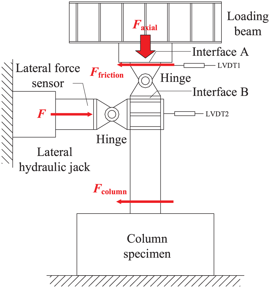
Typical quasi-static test setup for columns.

Strictly speaking, the direction of friction force is dependent on the direction of sliding or sliding tendency between the two sliding surfaces (see Figure 2). Thus, the total force obtained by the lateral force sensor is the superposition of the lateral friction force and the reaction force provided by the column specimen. It is hard to figure out the influence of frictional force only according to the magnitude of total lateral force. However, there are several signs in the raw hysteretic curve which indicate the existence of frictional force, including the linear unloading section with large stiffness and cusps (see Figure 2). The cusps are generally caused by the transition from static friction to sliding friction (or kinetic friction) and that explains why all the cusps appear shortly after the starting/termination points of lateral loading.

Figure 2.

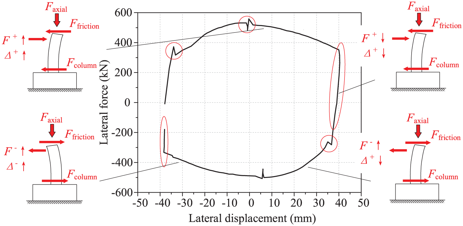
Influence of lateral friction force.

Test results from previous studies also showed similar phenomenon and indicated the existence of lateral friction force (Feng et al., 2018; Gu et al., 2010; Ma and Li, 2015; Ozcan et al., 2008; Wang et al., 2017). Different slip interface configurations, such as a PTFE–steel interface, a steel–steel interface (sliding tracks) and rollers, may affect the size of the cusps, but cannot totally eliminate this phenomenon, which makes the cusps a quite clear indicator of the lateral friction force. However, the magnitude of the lateral friction force and the proportion in total lateral force, which is rather implicit, is much more concerned during the test. It should be noted that friction force also develops in the pin and clevis of the axial and lateral hinges. However, friction force at these positions is quite small compared with the lateral friction force at the top. In this article, discussion and correction method is focused on the friction force at the sliding interface, while the influence of friction at the hinges is ignored.

Existing treatment methods on lateral friction force

In order to minimize the problem of lateral frictional force, many methods have been explored in previous studies. Some researchers modified the hysteretic loading device to reduce or even eliminate the influence of frictional force, while others tried to calculate or measure the value and development of frictional force, and make corrections during the data processing. In this section, these friction treatment methods are briefly reviewed and assessed.

Friction reduction treatment on sliding interface

The most common approach of reducing friction is to set a low-friction sliding device between the two slipping surfaces including sliding cart or steel rollers (Cai et al., 2017; Zhang and Wang, 2000), low-friction sliding track (Stephens et al., 2016), PTFE plate (Wu et al., 2017). This method is convenient and can be easily set up in nearly all kinds of loading devices. Besides, this method shows obvious effects on reducing friction for specimens under a low axial load since the friction coefficient could be reduced effectively. According to Table 1, it is noted that the steel rollers show a rather small friction coefficient, while a PTFE plate generally illustrates a higher friction coefficient. However, for specimens with a large cross-sectional area or with a large axial compression ratio, the influence of lateral friction is still non-negligible though the friction coefficient is rather small. And, the low wear resistance of PTFE can also affect the friction coefficient and aggravate the problem of lateral friction (Biswas and Vijayan, 1992). Moreover, the elastic or inelastic deformation of the steel rollers and sliding carts under large axial compression might also aggravate the problem of friction.

“Swing frame” loading device

Saatcioglu and Ozcebe (1989) used two vertical hydraulic jacks along with a loading beam to apply the axial load. Hinge joints were setup at the top and bottom of the column for each hydraulic jack. A “swing frame” was setup using all these devices and the lateral load was applied by a lateral hydraulic jack perpendicular to the frame plane as shown in Figure 3(a). A similar testing device was also adopted by other researchers (Jiang et al., 2019; Naqvi and El-Salakawy, 2016; Ozbakkaloglu and Saatcioglu, 2006; Yang, 2012). Similarly, posttensioned cables were also used to apply the axial loading of the column in order to avoid the influence of lateral friction force. The basic concern of this test setup is to avoid the interface sliding at the top. This test setup surely has an excellent performance of eliminating the influence of lateral friction. However, such method can be only used when the axial load is small enough (e.g. 600 kN for Saatcioglu and Ozcebe, 1989; 1750 kN for Yang, 2012; 1580 kN for Ozbakkaloglu and Saatcioglu, 2006; 550 kN for Naqvi and El-Salakawy, 2016). If the axial compression load is too large (e.g. 4459 kN for Bayrak and Sheikh, 1998; 5680 kN for Feng et al., 2018), axial actuator should be mounted on a much stronger reaction frame in order to provide such high axial compression force. Besides, P-delta effect will become a serious problem and excessive tilting may occur if the frame can rotate freely out of plane during the test, which could be dangerous if the specimen fails in brittle behavior.

Figure 3.

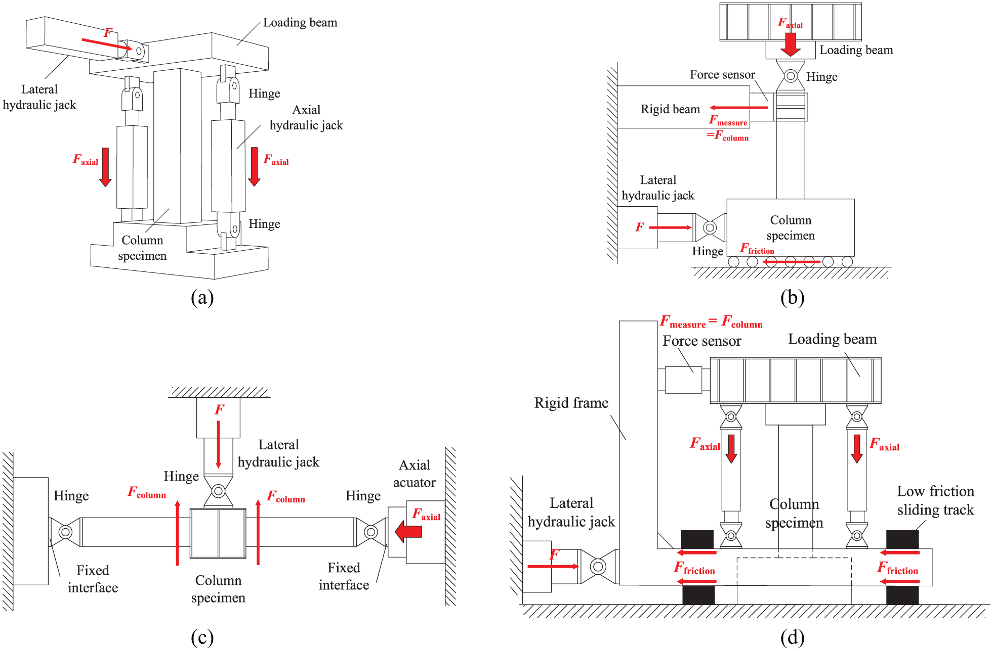
Test setups dealing with lateral friction force: (a) swing frame loading device, (b) friction eliminating test setup, (c) mid-span loading method, and (d) HNU-MUST system (Xiao et al., 2018).

Test setup of Sezen and Moehle (2006) is similar to the “Swing frame” device, while the rotation of the frame and applied lateral load was in the plane of the frame. This test setup avoids the danger of excessive out-of-plane displacement. However, due to the limitation of the axial hydraulic jack, rotation of the loading beam is fixed. The column specimen bends and fails in a double curvature shape, which requires a twice longer column specimen of the single curved one.

Friction eliminating test setup

Tao and Han (2001) came up with a new loading method (see Figure 3(b)). Rollers were setup below the specimen and lateral loading was applied at the bottom. A rigid lateral beam with a load sensor was setup at the top to limit the lateral displacement. Thus, the load obtained from the top lateral load sensor reflects exactly the column reaction force. However, this method requires significant modification to the test device. Difficulty may also exist for limiting the rotation of bottom rigid beam while keeping its lateral movement ability.

Xiao et al. (2018) proposed a test system named MUST (multiple usage structural testing equipment), which can maintain the axial loading to be perpendicular to the lateral loading and monitor the actual lateral forces applied to the specimen directly (see Figure 3(d)). Obviously, this loading system is a combination of the test setups of Sezen and Moehle (2006) and Tao and Han (2001). The actual reaction force of the column specimen can be recorded by the lateral force sensor mounted between the loading beam and the rigid frame. Influence of lateral friction at the sliding track can be totally eliminated.

Some researchers used alternative loading methods to reduce friction. One typical and useful method is constructing a specimen which consists of two symmetric columns and applying the lateral loading in the middle of the specimen, as shown in Figure 3(c) (Azizinamini et al., 1994; Fam et al., 2004; Guo and Lu, 2004; Lu and Lu, 2000; Matamoros and Sozen, 2003). According to the symmetry of the specimen, no lateral friction force that may influence the measurement of the lateral force exists. Technically, friction can be totally eliminated using this method. This method reduces the friction by the symmetry effect of the specimen, so imperfection in the specimen construction and experiment setup (e.g. asymmetry) may cause deviation of the experiment result. Moreover, a block with a large mass needs to be arranged in the middle of the specimen, which can be quite risky due to the large P-delta effect.

Calculation of lateral friction force

There are also some researchers making efforts to calculate the lateral friction during the test and then make corrections during data processing. Zhang et al. (2015) used two additional linear variable differential transformers (LVDTs) at the top and bottom of the sliding interface to measure the slipping displacement. An empirical friction coefficient of 0.527% was used to calculate the friction force. This method involves only work in data processing and can save much time and money on the modification of the test device or specimens. However, the accurate determination of friction coefficient is not an easy task considering that the friction force may be influenced by many factors during the test, including interface materials, axial load, lateral loading speed, lateral displacement, temperature, and lubrication. The validity of using the same constant friction coefficient for various cases remains uncertain.

Measurement of lateral friction force

Shear force measurement device

In order to measure the development process of lateral friction force directly for different column specimens, especially large-size ones, a shear force measurement device, which is capable of measuring shear force around 300 kN under an axial load around 20,000 kN, is needed in this article. Different kinds of shear measurement devices have been proposed and some of them have been used in structural experiment measurement (Canbay et al., 2004; Liang et al., 2010; Liu and Tzo, 2002; Suresh and Tjin, 2005; Sanders, 1995). However, measurement device which meets the requirement above is extremely rare in both the literature and markets.

In this way, a simple novel shear force measurement device proposed by the Pan et al. (2017) is presented in this article. This device consists of an upper plate, a lower plate, and several vertical deformable steel plates. A group of four strain gauges was mounted on each vertical plate as shown in Figure 4. All the vertical steel plates are parallel and equidistant to each other, which are used to transmit the vertical and shear force. Vertical plates should be designed to be strong enough so that the steel maintains in the elastic stage during the experiment.

Figure 4.

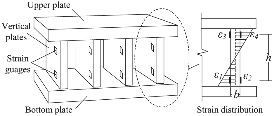
Details of the shear force measurement device.

For each vertical plate, under vertical and lateral force, strains obtained by the strain gauges near the lower plate are denoted as ε₁ and ε₂, respectively, and those near the upper plate are denoted as ε₃ and ε₄, respectively, as shown in Figure 4. The total lateral shear force applied on this device can be calculated from the four strains using the following equation

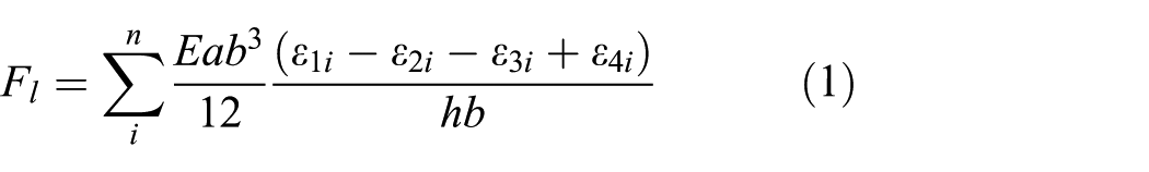
F_{l} = \sum_{i}^{n} \frac{Ea b^{3}}{12} \frac{(ε_{1 i} - ε_{2 i} - ε_{3 i} + ε_{4 i})}{hb}

(1)

where n is the number of vertical plates, E is the elastic modulus of steel, a is the width of the plates, b is the thickness of the plates, and h is the distance between the upper and lower strain gauges.

A real shear force measurement device has been manufactured and used during real tests in Tsinghua University. In order to prove the accuracy and stable performance of the proposed shear force measurement device, a calibration test was carried out. Two identical measurement devices were fixed to the top and bottom of a conjunction steel block (see Figure 5(a)). Different levels of axial load were applied to the measurement devices first and reverse lateral load of 400 kN was applied to the steel block subsequently. In this way, a combined axial force and ±200 kN lateral force was applied to each measurement device. Figure 5(b) illustrated the relationship between the applied lateral load and the measured lateral load calculated by equation (1). It can be seen that the measured force showed a very fair agreement with the applied load and the curves coincide well with each other under different axial load levels, indicating a stable and consistent measurement performance. From test results, the maximum relative error of the shear force measured by the device and the lateral load sensor on the hydraulic jack is less than 3.7%.

Figure 5.

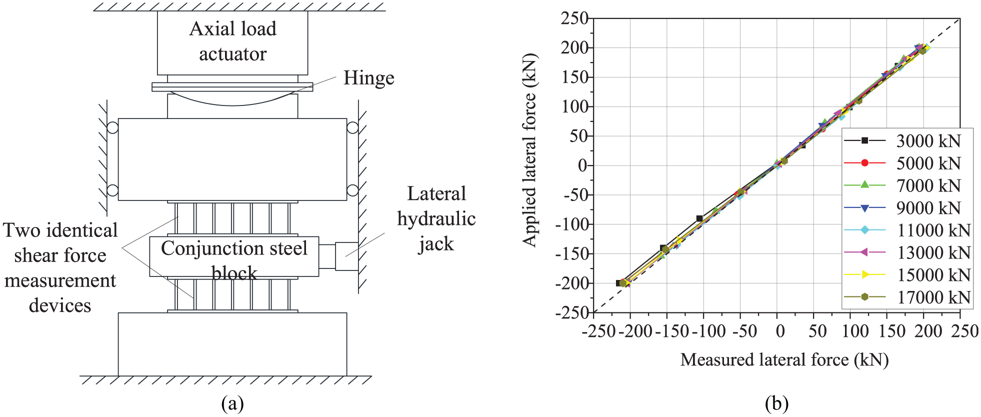
Calibration of the new shear force measurement device: (a) calibration test setup and (b) calibration test results.

Friction force measured in real tests

Using this device at the sliding interface A (see Figure 1), the lateral friction force can be obtained during the experiment. And the real reaction force of the column specimen can be calculated by subtracting the lateral force measured by the device from the total lateral force measured by lateral force sensor.

Test results of four column specimens including two steel-concrete-FRP-concrete columns (SCFC-1 and SCFC-2) (Feng et al., 2015), one FRP-wrapped RC column (FRC-1), and one concrete-filled FRP tube columns (CFFT-1 and CFFT-2) were selected and presented. All the loading devices of the four specimens were equipped with a PTFE–steel sliding interface. Lateral friction force of these specimens was also measured during the test. Details of the test information and the average lateral friction force are summarized in Table 2. Figure 6(a) shows the raw total lateral force–displacement hysteretic curve obtained from the experiment as well as the hysteretic curve after friction elimination. It can be seen that after the adjustment, the cusps caused by lateral friction are actually eliminated. It is also evident that the influence of friction force is significant, which can reach up to around 30% of the total measured lateral force. Hysteretic curves of lateral friction force measured by the device are also illustrated in Figure 6(b).

Table 2.

Validation of the friction correction method.

Specimen	F_axial (kN)	Axial pressure (MPa)	Measured friction force (kN)	Friction coefficient ratio	Parameters in the friction model				Relative error of f_s (%)
					f_s (kN)	f _max (kN)	f _Δ (kN)	E_f (kN/mm)
SCFC-1	6850	4.76	200.1	2.9	173.0	253.0	72.3	94.9	−13.5
SCFC-2	6047	4.20	128.3	2.1	144.3	196.2	63.7	61.2	12.5
FRC-1	3910	2.71	102.5	2.6	117.0	231.3	48.5	94.6	14.1
CFFT-1	530	2.12	18.8	3.5	15.3	17.3	4.0	10.7	−18.7

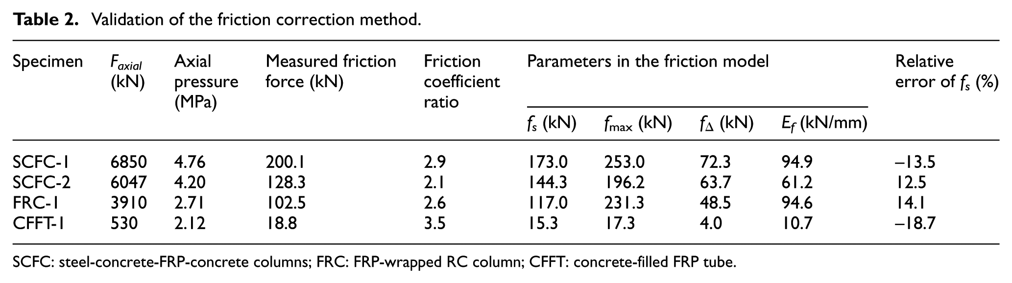
SCFC: steel-concrete-FRP-concrete columns; FRC: FRP-wrapped RC column; CFFT: concrete-filled FRP tube.

Figure 6.

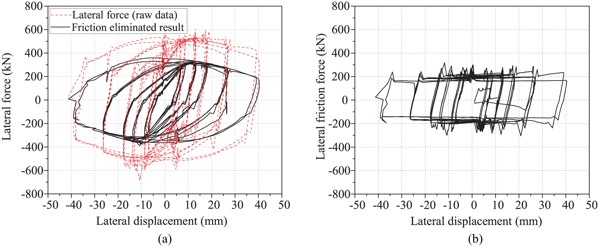
Friction measurement results of SCFC-1: (a) hysteretic curves of raw data and friction eliminated result and (b) hysteretic curves of lateral friction force.

Friction development process

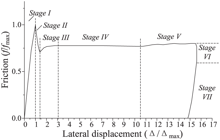
Due to the symmetry of the hysteretic curve of lateral friction force and similar friction hysteretic behavior of different sliding interface configuration, half of a typical hysteretic loop of SCFC-1 with a PTFE-steel interface is illustrated in Figure 7. Many studies on the friction behavior at the PTFE-steel interface of seismic isolators also illustrated a quite similar friction hysteretic behavior due to a similar load pattern and motion progress of the interface (Bondonet and Filiatrault, 1997; Dolce et al., 2005).

Figure 7.

Typical friction behavior.

During the quasi-static tests, the slip between the loading beam and the axial hinge experienced a static–accelerating–uniform motion process. According to the different motion states, the friction–lateral displacement curve can be divided into seven stages.

Stage 1 “Pre-sliding stage”: during this stage, there is no relative movement, but there is slipping tendency at the interface. And, the lateral friction force shows an almost linear relationship with lateral displacement until the maximum friction force (f_max). Technically, the lateral displacement should be equal to zero during this stage since there is no relative movement at the interface. However, the lateral displacement is obtained from an LVDT sensor mounted at the top of the column specimen (i.e. LVDT2 in Figure 1). As a result, although there is no slipping at interface A in Figure 1, the lateral displacement measured at the top of the column is not zero because of the elastic deformation of the axial loading device, rotation of the vertical hinge, and deformation of the column specimen.

Stage 2 “Stribeck friction stage”: interface slipping occurs in this stage. Stribeck found that the friction force decreases with the increasing slipping velocity after the maximum static friction force which is also known as negative viscous friction or “Stribeck friction” (Armstrong-Hélouvry, 2012). When the slip speed accelerates to a certain level and exceeds the velocity limitation of Stribeck friction, friction force begins to increase. The existence of stage 2 causes a cusp at the very beginning of friction curves.

Stage 3 “Viscous friction stage”: after stage 2, the lateral loading speed has not reached the preset loading speed and still stays in the acceleration motion stage. The friction force begins to increase with the increasing lateral loading speed due to the viscous property of PTFE plate of the slipping interface. This phenomenon has also been found by several researchers (Constantinou et al., 1990; Mokha et al., 1991).

Stage 4 “Steady slip stage”: when the loading speed reaches the preset speed, the lateral loading head moves at a constant speed and the friction force remains constant (f_s) with the increase in the displacement.

Stage 5 “Unstable decelerating stage”: when the lateral displacement approaches the preset value where unloading begins, the lateral loading speed begins to decelerate and leads to a slight increase in the friction force. Due to the unpredictable decelerating process, the unstable decelerating stage may show fluctuations or cusps.

Stage 6 “Friction resilience stage”: after the lateral loading completely stopped, the friction force has a sudden decrease. This phenomenon is caused by the recovery of elastic deformation of the axial loading device which cannot be measured by the LVDTs.

Stage 7 “Unloading stage”: during this stage, there is no slip at the interface. The lateral loading jack begins to move reversely and the friction force begins to decrease with the decrease in the lateral displacement with a constant stiffness approximately equal to that of stage 1. The apparent friction force equals the elastic force of the axial loading device until slip starts in the opposite direction.

Friction model and friction correction method

As discussed above, the shear measurement device is capable to measure the lateral friction force accurately and eliminate the influence of friction in the test result. However, the manufacture and calibration of this device will surely cause additional expense and time. In this way, a prediction model of the lateral friction force in quasi-static tests of columns and a correction method is proposed in this section, which can be used to predict the development of friction and eliminate its influence in tests when the shear force measurement device is not used.

Many theoretical models for friction have been proposed by previous researchers in the field of mechanical engineering (Armstrong-Hélouvry, 2012) including static friction models and dynamic ones, which relate the friction force with either the interface sliding velocity (Armstrong-Hélouvry et al., 1994; Karnopp, 1985) or slipping displacement (Haessig and Friedland, 1991). However, neither of the two types of friction models is proper for friction correction in this article because of the difficulties in parameter calibration or high computing complexity. In structural engineering area, several friction models have been proposed for seismic isolation sliding bearings under seismic load (Chang et al., 1990; Nouri, 2004; Tsai, 1997), among which a quite well-established friction model was proposed by Lomiento et al. (2013). Influence of axial load, cycle numbers, and velocity was considered in this model. The model proposed by Lomiento et al. (2013), like almost all the friction models for sliding isolation devices, does not include the contribution of static friction (i.e. the friction force corresponding to the “cusp” in the hysteretic curve). An improved model accounting for static friction has also been presented by Gandelli et al. (2019). However, additional test should be carried out to determine some parameters in the model beforehand (e.g. “slow motion coefficient of friction” of Lomiento et al., 2013), which is a crucial threshold of adopting such models in the present case. Moreover, the different application environment also causes some deviations between this model and actual friction behavior in quasi-static tests.

According to the friction force development process obtained from the test, a simplified theoretical friction development model is proposed in this article which is convenient for the calculation and correction of friction force during data processing. Parameters in this model can be calibrated according to the raw hysteretic curves obtained from the test for each individual specimen.

Theoretical friction model

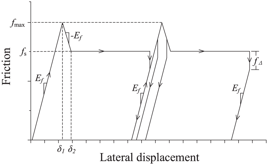
A simple friction model for quasi-static tests is proposed and illustrated in Figure 8.

Figure 8.

Theoretical friction model.

The loading stage of the model consists of three linear stages. The pre-slipping stage is simulated by the first linear stage with a constant friction stiffness E_f and is terminated at the maximum static friction force f_max; this is followed by the second stage, in which the friction force decreases with the lateral displacement at a rate of E_f (i.e. the Stribeck friction behavior); the second stage is terminated at the stable sliding friction force f_s. The third linear stage with a constant friction force f_s simulates the stable sliding stage. The viscous friction stage is ignored since that it is hard to predict the development of friction force in this stage and that it has little influence on the overall test result.

For the unloading stage, the unloading pattern is simulated by the same behavior of the loading pattern no matter at which stage the unloading begins. The unloading stage consists of a friction resilience with magnitude f_△ and a linear friction unloading stage with a stiffness E_f.

Calibration method of the parameters

In this model, four individual parameters need to be determined, namely, the friction stiffness E_f, the maximum static friction f_max, the stable sliding friction f_s, and the friction resilience f_Δ. All these parameters can be calibrated using only the raw data obtained by the existing measurement device in the experiment. No adjustment of test equipment or additional measurement device is needed.

Friction resilience f_Δ

For a hysteretic curve of a column specimen, assume that there are total n hysteretic loops in the curve. Before the calibration of all the parameters, it is necessary to determine the kth hysteretic loop where the first cusp appears, which indicates the reach of maximum friction force. Before the kth loop, lateral friction force remains to be in a linear relationship with displacement. And, the lateral displacement is quite small and the major part of the specimen columns generally remains elastic. In this way, the shapes of the hysteretic loops of total lateral force and friction force are nearly parallelograms (see Figure 9(a)).

Figure 9.

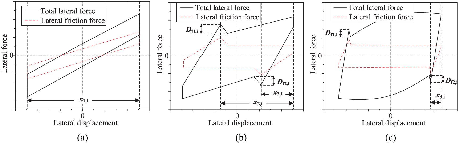
Calibration method of parameters in friction model: (a) first to (k– 1)th hysteretic loops, (b) kth hysteretic loop, and (c) (k+ 1)th to nth hysteretic loops.

In order to calibrate parameter f_Δ, all the hysteretic loops from the first loop to the (k– 1)th loop should be selected. The friction resilience f_Δ can be calculated by the following equation

f_{Δ} = \frac{\sum_{1}^{k - 1} \frac{A_{i} S_{i}}{x_{1, i}}}{k - 1}

(2)

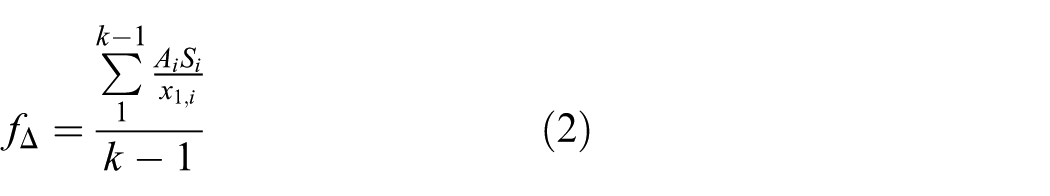
where x_1,i is the range of the lateral displacement, S₁ is hysteretic loop area, and A_i is friction hysteretic energy proportion parameter of ith loop, which defined as the percentage of the friction hysteretic energy in the whole measured hysteretic energy.

Figure 10 shows the development of parameter A with the lateral displacement of the four specimens presented in this study and three SCFC specimens tested before (Feng et al., 2018). It is indicated that A remains almost constant at small displacements, then decreases with the increasing displacement afterward. In particular, when the lateral displacement is smaller than 10 mm (after the kth loop and shortly before the peak point of the specimen), the value of A generally lies between 52% and 62% (see Figure 10).

Figure 10.

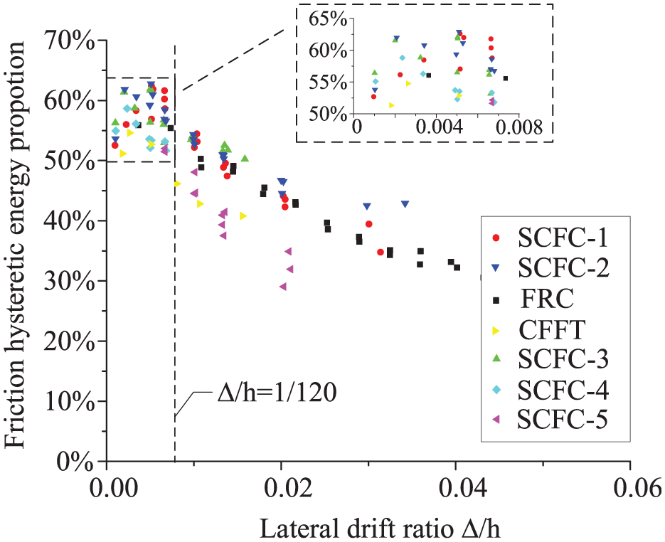
Friction hysteric energy proportion development.

In this way, as long as the maximum displacement in the kth loop is smaller than the displacement corresponding to peak point, an empirical constant value of 0.55 is recommended for parameters A₁–A_k.

Stable sliding friction force, f_s

The stable sliding friction force f_s is the most important parameter in this theoretical model because it has the largest influence on the value and shape of the friction hysteretic loops. The kth loop should be selected to determine this parameter, considering that the cusp is the indicator of the maximum friction force (see Figure 9(b)). The stable sliding friction force f_s can be calculated using the following equation

f_{s} = A_{k} \cdot \frac{S_{2, k}}{2 x_{2, k}}

(3)

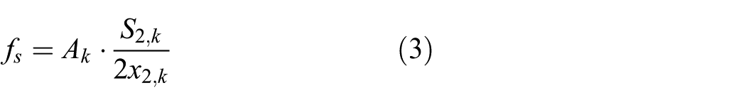
where x_2,k is the displacement range from the vertex of the cusp to the unloading beginning point, S_2,k is the area of total hysteretic loop, and A_k is the friction hysteretic energy proportion of kth loop.

It is noted that the parameter f_s is calibrated only by raw data of a single hysteretic loop, which is easily be affected by the experimental bias. Besides, if the maximum displacement of the kth loop is too large, the parameter A_k would be smaller than the recommended value and cause some deviation on the calibrated f_s. In order to address this issue, two to three load loops are recommended to be done at the same lateral displacement level equal to that of the kth loop, and the mean value of f_s calibrated by these loops should be used in the following calculation. Meanwhile, the unloading of kth loop is recommended to be done shortly after the first cusp appears. A smaller value of x_2,k will lead to a more accurate f_s.

Maximum static friction, f_max

From the test result and the discussion above, it is indicated that the cusp is totally caused by the influence of lateral friction force, which means that the difference between the top and bottom of the cusp in the whole hysteretic loops is equal to that in friction force hysteretic loops. The maximum static friction f_max can be calculated by the following equation

f_{max} = f_{s} + \frac{\sum_{k}^{n} (D_{f 1, i} + D_{f 2, i})}{n - k + 1}

(4)

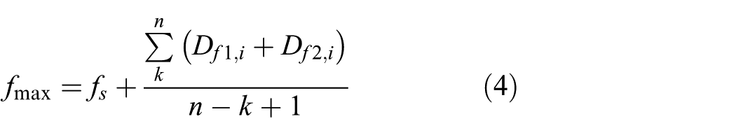
where f_s is the stable sliding friction force calculated, D_f_1,i and D_f_2,i is the difference of the top and bottom of the cusps at initial loading and reversely loading in ith hysteretic loop, respectively (see Figure 9(b) and (c)).

Friction stiffness, E_f

Technically, every hysteretic loop can be selected to calibrate the parameter E_f. However, the last and the second last of all the hysteretic loops are recommended since the linear stage of these loops is quite long and the lateral force range of the linear stage is large. Besides, the friction force is fully developed and is relatively stable, which is beneficial for calibration of the friction stiffness. The friction stiffness E_f can be calculated by the following equation

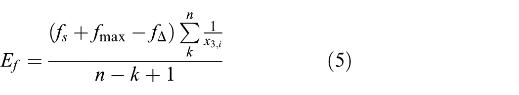
E_{f} = \frac{(f_{s} + f_{max} - f_{Δ}) \sum_{k}^{n} \frac{1}{x_{3, i}}}{n - k + 1}

(5)

where f_s is the calculated stable sliding friction force, f_max is the maximum friction force, f_Δ is friction resilience value, and x_3,i is displacement range of the linear unloading and reversely loading stage of ith hysteretic loop (see Figure 9(b) and (c)).

Friction correction using the proposed model

Based on the theoretical friction model above, procedure of the friction correction method for quasi-static tests can be proposed as follows:

Separate each single hysteretic loop from the whole experimental lateral displacement–load curve (test hysteretic curve) of the specimen. One single hysteretic loop consists of a loading–unloading cycle and a reverse loading–unloading cycle.

Calibrate the four individual parameters (f_Δ, f_max, f_s, and E_f) by the method discussed above.

For each individual test hysteretic loop, determine the key points of different stages, such as the beginning point of the loading stage, beginning and terminating points of the unloading stage. These key points in test hysteretic loop also correspond to those in the friction hysteretic loop.

Determine the corresponding friction force for each lateral displacement of the test hysteretic loop. Make the friction correction by subtracting the friction force from the whole lateral force. The so-obtained curve may need to be smoothened to eliminate cusps that have not been totally corrected.

Put all the individual corrected hysteretic loops together and get the actual hysteretic curve of the column specimen.

Validation and examples of the friction correction method

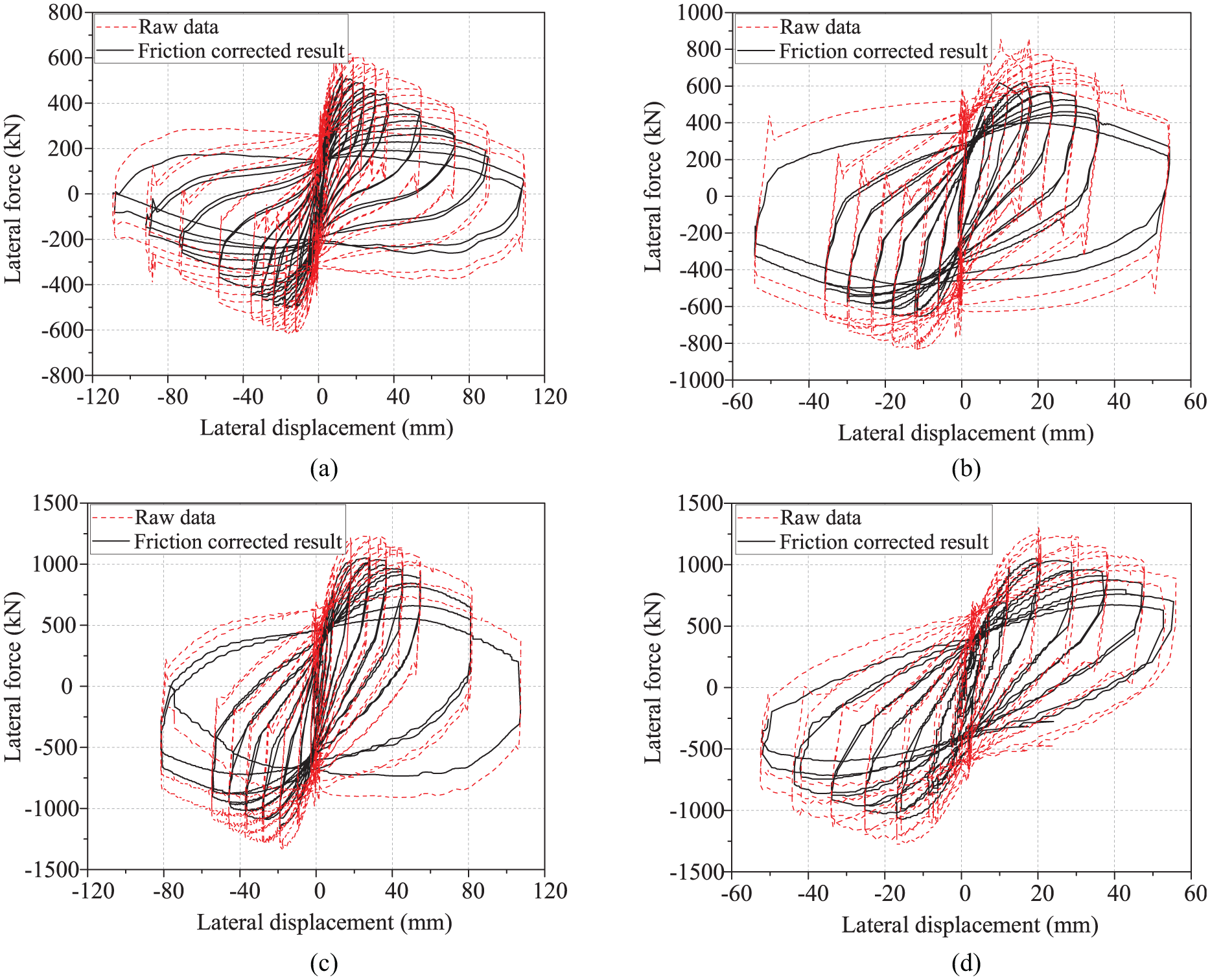
The proposed friction correction method has been carried out for four column specimens tested using loading device with a PTFE–steel sliding interface. Parameters of the corresponding friction model were calculated using the raw test data of the four columns and listed in Table 2. And, the relative error of the calibrated friction force f_s and the average measured friction force is also calculated and listed in Table 2. It is obvious that the parameter f_s shows a reasonable estimation of the real value measured in tests. Figure 11 shows the comparison between the hysteretic curves after friction elimination using the friction force measured during test and the one calculated using the proposed model of the four columns. It can be seen that the two friction-corrected curves show a fair agreement with each other for each group.

Figure 11.

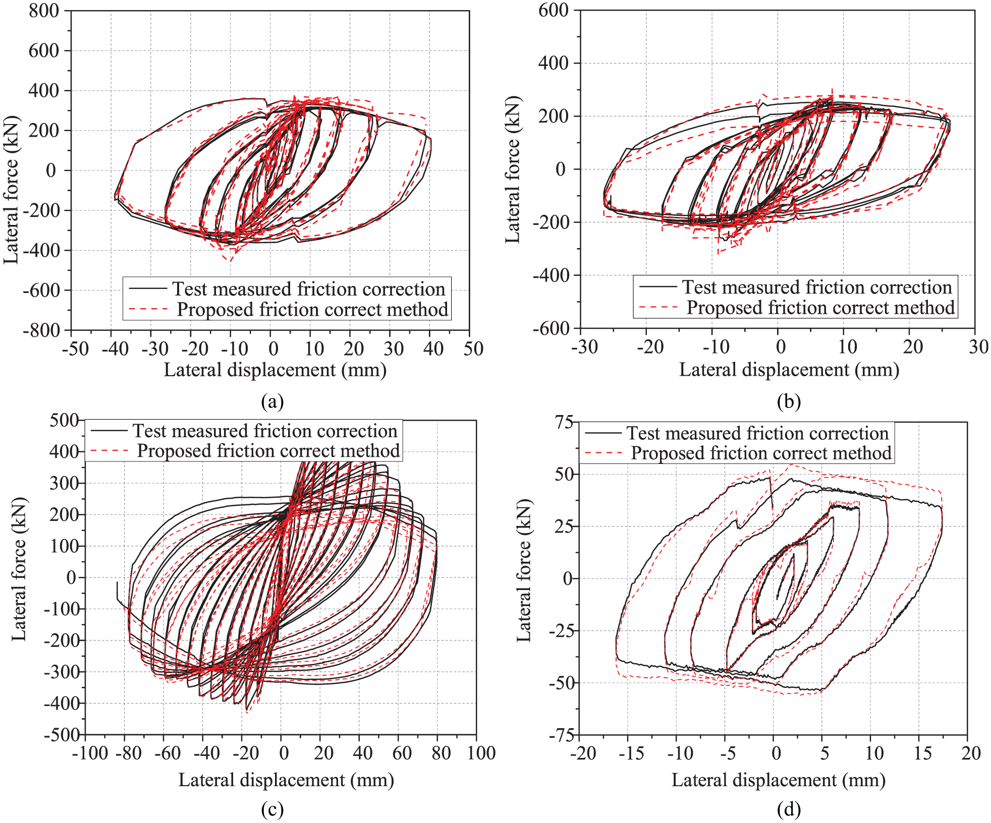
Comparison of the friction-corrected hysteretic curves: (a) SCFC-1, (b) SCFC-2, (c) FRC-1, and (d) CFFT-1.

Figure 12 shows the friction development curve in different hysteretic loops of SCFC-1. Obviously, the friction development curve calculated by the theoretical model is in good agreement with the test results, especially for hysteretic loops at relatively large displacements. Deviation may occur in hysteretic loops near the points where cusps first appear (e.g. Loop 2 in Figure 12) because of the interaction of the Stribeck friction stage, unstable decelerating stage, and friction resilience stage at that time.

Figure 12.

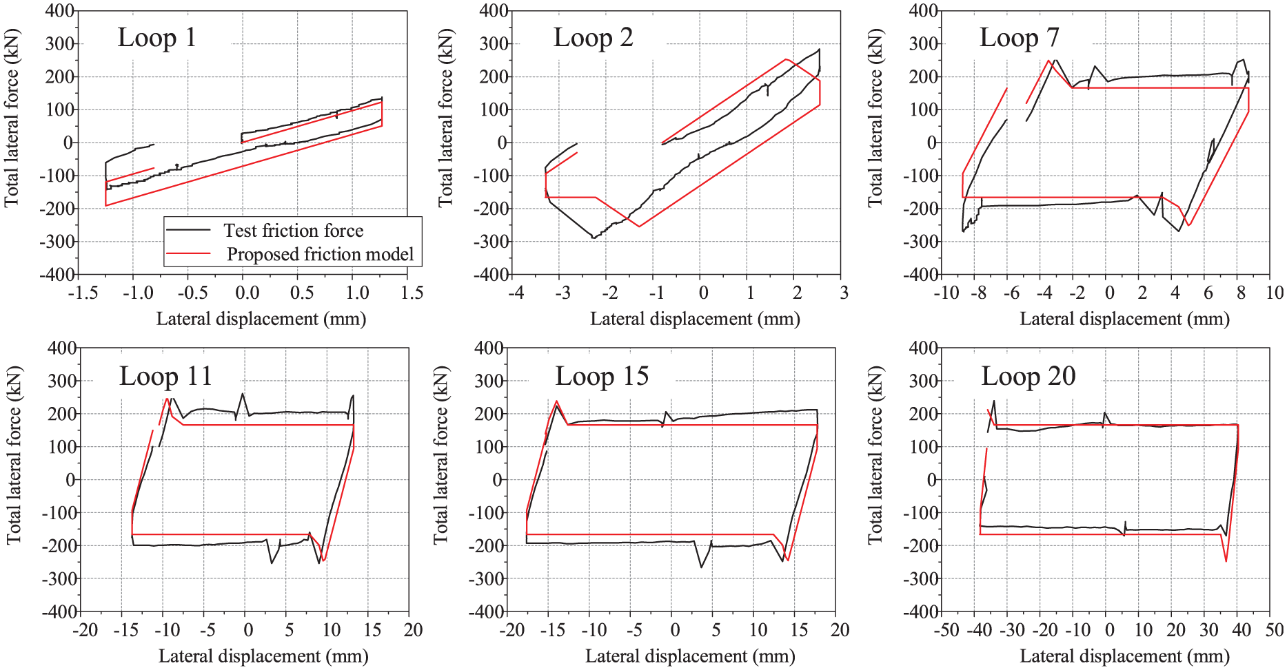
Comparison of the friction development of SCFC-1.

It should be noted that the proposed friction correction method shows reasonable results in lateral friction estimation and elimination for columns in quasi-static tests with a PTFE–steel interface. For other sliding interface types including rollers and steel sliding track (steel–steel interface), the proposed model and friction correction method should be further validated to be adopted.

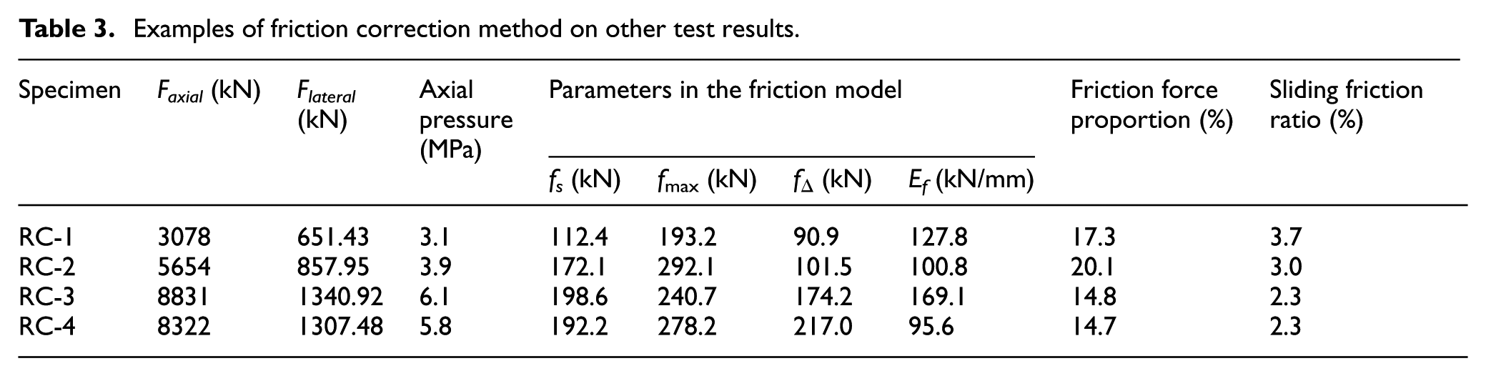
Examples using raw test results of four reinforced concrete columns were carried out in order to further illustrate the influence of lateral friction force. Four specimens were tested on the same loading device with a PTFE–steel interface. Details results of tests and friction correction procedure are listed in Table 3. The original test results and friction-corrected results are presented in Figure 13.

Table 3.

Examples of friction correction method on other test results.

Specimen	F_axial (kN)	F_lateral (kN)	Axial pressure (MPa)	Parameters in the friction model				Friction force proportion (%)	Sliding friction ratio (%)
				f_s (kN)	f _max (kN)	f _Δ (kN)	E_f (kN/mm)
RC-1	3078	651.43	3.1	112.4	193.2	90.9	127.8	17.3	3.7
RC-2	5654	857.95	3.9	172.1	292.1	101.5	100.8	20.1	3.0
RC-3	8831	1340.92	6.1	198.6	240.7	174.2	169.1	14.8	2.3
RC-4	8322	1307.48	5.8	192.2	278.2	217.0	95.6	14.7	2.3

Figure 13.

Examples of friction correction method: (a) RC-1, (b) RC-2, (c) RC-3, and (d) RC-4.

From the friction correction results of the columns, the unloading section with a large stiffness and cusps can be eliminated. The calculated results of the proportion of the lateral friction force to the total lateral force of the specimens ranged from 14.7% to 38.9%, which indicates the great influence of the friction force on the test results. According to the friction correction results, the same loading device may also show different friction ratio with different column specimen tested (see Table 3) due to different axial pressure on the sliding interface. In this way, an empirical sliding friction ratio of a certain loading device is not reliable and might only be adopted when the axial pressure, loading scheme, and test environment (i.e. temperature) are similar.

Conclusion

This article presents a study aiming to predict the lateral friction forces existing in quasi-static tests of structural columns. Previous treatments on the lateral friction force by existing research were first summarized and discussed. A shear force measurement device was constructed and used for friction measurement during quasi-static tests. The development of lateral friction force with the loading process was obtained from a real test. A simple model to predict the friction force in quasi-static tests with a PTFE-steel sliding interface, based on which a procedure of friction correction method was proposed. Finally, some examples of the friction correction method were carried out, which verified the validity of this method. Based on the results and discussion presented in this article, the following conclusions can be drawn:

The shear force measurement device proposed by Pan et al. (2017) can be used for measurement of friction forces in quasi-static tests. The friction hysteretic curve can be easily and accurately obtained using the device, which can then be used to correct the overall hysteretic curve obtained from the tests. Cusps and fluctuation on the hysteretic curve caused by friction can be well eliminated.

The simple friction model proposed in this article generally provides close predictions of the friction hysteretic curve. Hysteretic curve after friction correction using the model shows good agreement with the test results. For specimens without friction measurement during the test, the influence of friction force can be well corrected using the model. However, this model is only validated by test with a PTFE–steel sliding interface and should be further calibrated when adopted for other interface type (e.g. steel–steel interface).

For the first several hysteretic loops, the development of friction force predicted by the proposed model somewhat deviates from the test result, especially near the hysteretic loop where cusps first appear. However, for the hysteretic loops at large displacements, the development of friction force predicted by the model shows much better coincidence with the test result since that the friction force is more fully developed and the effect of the unstable section of friction is smaller.

Cusps appearing during the loading section due to the pause of the loading is hard to be corrected using the proposed friction correction method, but can be well eliminated by smoothing the corrected curves.

In future quasi-static tests, several load cycles at lateral displacements near the first occurrence of cusps are recommended in order to calibrate the parameters of the proposed model more precisely. Besides, an empirical sliding friction ratio can also be adopted as a reference in the friction correction for specimens with similar section configuration and axial load tested using same loading frame.

Footnotes

Declaration of Conflicting Interests

The author(s) declared no potential conflicts of interest with respect to the research, authorship, and/or publication of this article.

Funding

The author(s) disclosed receipt of the following financial support for the research, authorship, and/or publication of this article: This research was supported by the National Key Program of China (2017YFC 0703005) and the National Natural Science Foundation of China (Nos 51661165016, 51522807, and 51778330).

ORCID iD

Peng Feng

References

Armstrong-Hélouvry

(2012) Control of Machines with Friction. vol. 128. New York: Springer.

Armstrong-Hélouvry

Dupont

De Wit

(1994) A survey of models, analysis tools and compensation methods for the control of machines with friction. Automatica 30(7): 1083–1138.

Azizinamini

Kuska

SSB

Brungardt

, et al. (1994) Seismic behavior of square high-strength concrete columns. Structural Journal 91(3): 336–345.

Bayrak

Sheikh

(1998) Confinement reinforcement design considerations for ductile HSC columns. Journal of Structural Engineering 124(9): 999–1010.

Biswas

Vijayan

(1992) Friction and wear of PTFE—a review. Wear 158(1–2): 193–211.

Bondonet

Filiatrault

(1997) Frictional response of PTFE sliding bearings at high frequencies. Journal of Bridge Engineering 2(4): 139–148.

Cai

Wang

(2017) Full-scale seismic testing of concrete building columns reinforced with both steel and CFRP bars. Composite Structures 178: 195–209.

Canbay

Ersoy

Tankut

(2004) A three component force transducer for reinforced concrete structural testing. Engineering Structures 26(2): 257–265.

Chang

Hwang

Lee

(1990) Analytical model for sliding behavior of Teflon-stainless steel interfaces. Journal of Engineering Mechanics 116(12): 2749–2763.

10.

Constantinou

Mokha

Reinhorn

(1990) Teflon bearings in base isolation II: modeling. Journal of Structural Engineering 116(2): 455–474.

11.

Dolce

Cardone

Croatto

(2005) Frictional behavior of steel-PTFE interfaces for seismic isolation. Bulletin of Earthquake Engineering 3(1): 75–99.

12.

Fam

Qie

Rizkalla

(2004) Concrete-filled steel tubes subjected to axial compression and lateral cyclic loads. Journal of Structural Engineering 130(4): 631–640.

13.

Feng

Cheng

(2018) Seismic performance of hybrid columns of concrete-filled square steel tube with FRP-confined concrete core. Journal of Composites for Construction 22(4): 4018015.

14.

Feng

Cheng

Bai

, et al. (2015) Mechanical behavior of concrete-filled square steel tube with FRP-confined concrete core subjected to axial compression. Composite Structures 123: 312–324.

15.

Gandelli

Penati

Quaglini

, et al. (2019) A novel OpenSees element for single curved surface sliding isolators. Soil Dynamics and Earthquake Engineering 119: 433–453.

16.

, et al. (2010) Confinement effectiveness of FRP in retrofitting circular concrete columns under simulated seismic load. Journal of Composites for Construction 14(5): 531–540.

17.

Guo

(2004) Experimental study on the hysteretic model of RC columns with high axial compressive ratio. China Civil Engineering Journal 37: 5–31 (in Chinese).

18.

Haessig

Friedland

(1991) On the modeling and simulation of friction. Journal of Dynamic Systems, Measurement, and Control 113(3): 354–362.

19.

(2010) Behaviour and modelling of FRP-confined hollow and concrete-filled steel tubular columns. Doctoral Dissertation, The Hong Kong Polytechnic University, Kowloon, Hong Kong.

20.

Jiang

(2014) Plastic hinge length of FRP-confined square RC columns. Journal of Composites for Construction 18(4): 04014003.

21.

Jiang

Yuan

, et al. (2019) Effect of interfacial bond on plastic hinge length of FRP-confined RC columns. Journal of Composites for Construction 23(2): 04019007.

22.

Karnopp

(1985) Computer simulation of stick-slip friction in mechanical dynamic systems. Journal of Dynamic Systems, Measurement, and Control 107(1): 100–103.

23.

Leon

Deierlein

(1996) Considerations for the use of quasi-static testing. Earthquake Spectra 12(1): 87–109.

24.

Liang

Zhang

Song

, et al. (2010) Design and fabrication of a six-dimensional wrist force/torque sensor based on E-type membranes compared to cross beams. Measurement 43(10): 1702–1719.

25.

Liu

(2016) The development and application of a new measure equipment of shear force. Doctoral Dissertation. Tsinghua University, Beijing, China (in Chinese).

26.

Liu

Tzo

(2002) A novel six-component force sensor of good measurement isotropy and sensitivities. Sensors and Actuators A: Physical 100(2–3): 223–230.

27.

Lomiento

Bonessio

Benzoni

(2013) Friction model for sliding bearings under seismic excitation. Journal of Earthquake Engineering 17(8): 1162–1191.

28.

(2000) Seismic behavior of concrete-filled rectangular steel tubular columns under cyclic loading. Journal of Building Structures 21: 2–11 (in Chinese).

29.

(2015) Experimental study of the seismic behavior of predamaged reinforced-concrete columns retrofitted with basalt fiber-reinforced polymer. Journal of Composites for Construction 19(6): 04015016.

30.

Matamoros

Sozen

(2003) Drift limits of high-strength concrete columns subjected to load reversals. Journal of Structural Engineering 129(3): 297–313.

31.

Mokha

Constantinou

Reinhorn

(1991) Further results on frictional properties of teflon bearings. Journal of Structural Engineering 117(2): 622–626.

32.

Naqvi

El-Salakawy

(2016) Lap splice in GFRP-RC rectangular columns subjected to cyclic-reversed loads. Journal of Composites for Construction 21(4): 04016117.

33.

Nouri

(2004) Friction identification in mechatronic systems. ISA Transactions 43(2): 205–216.

34.

Ozbakkaloglu

Saatcioglu

(2006) Seismic behavior of high-strength concrete columns confined by fiber-reinforced polymer tubes. Journal of Composites for Construction 10(6): 538–549.

35.

Ozcan

Binici

Ozcebe

(2008) Improving seismic performance of deficient reinforced concrete columns using carbon fiber-reinforced polymers. Engineering Structures 30(6): 1632–1646.

36.

Pan

Liang

Deng

, et al. (2017) A new shear measurement device and measuring method. Patent CN104483046B, China (in Chinese).

37.

Saatcioglu

Ozcebe

(1989) Response of reinforced concrete columns to simulated seismic loading. Structural Journal 86(1): 3–12.

38.

Sanders

(1995) Interface mechanics in external prosthetics: review of interface stress measurement techniques. Medical and Biological Engineering and Computing 33(4): 509–516.

39.

Sezen

Moehle

(2006) Seismic tests of concrete columns with light transverse reinforcement. ACI Structural Journal 103(6): 842–849.

40.

Stephens

Lehman

Roeder

(2016) Design of CFST column-to-foundation/cap beam connections for moderate and high seismic regions. Engineering Structures 122: 323–337.

41.

Sun

Zhang

, et al. (2017) Experimental study on concrete columns reinforced by hybrid steel-fiber reinforced polymer (FRP) bars under horizontal cyclic loading. Construction and Building Materials 130: 202–211.

42.

Suresh

Tjin

(2005) Effects of dimensional and material parameters and cross-coupling on FBG based shear force sensor. Sensors and Actuators A: Physical 120(1): 26–36.

43.

Tao

Han

(2001) Tests of hysteresis behaviors of concrete filled steel tubular beam-columns with square sections. Earthquake Engineering and Engineering Vibration 1: 74–78 (in Chinese).

44.

Tsai

(1997) Finite element formulations for friction pendulum seismic isolation bearings. International Journal for Numerical Methods in Engineering 40(1): 29–49.

45.

Wang

Huang

, et al. (2017) Seismic performance of CFRP-retrofitted large-scale square RC columns with high axial compression ratios. Journal of Composites for Construction 21(5): 04017031.

46.

Pan

RKL

, et al. (2017) Seismic behavior of steel reinforced ECC columns under constant axial loading and reversed cyclic lateral loading. Materials and Structures 50(1): 78.

47.

Xiao

Sun

, et al. (2018) Development and validation of earthquake simulation testing equipment MUST for large-scale structural components. Journal of Building Structures 39(6): 149–157 (in Chinese).

48.

Yang

(2012) Flexural behaviour of RC columns using wire ropes as lateral reinforcement. Magazine of Concrete Research 64(3): 269–281.

49.

Zhang

Teng

(2015) Experimental behavior of hybrid FRP-concrete-steel double-skin tubular columns under combined axial compression and cyclic lateral loading. Engineering Structures 99: 214–231.

50.

Zhang

Wang

(2000) Seismic behavior of reinforced concrete shear walls subjected to high axial loading. Structural Journal 97(5): 739–750.

Friction measurement and correction method in quasi-static tests of columns under combined axial and cyclic lateral loading

Abstract

Keywords

Introduction

Influence of lateral friction force and treatment methods

Characteristics of lateral friction force

Existing treatment methods on lateral friction force

Friction reduction treatment on sliding interface

“Swing frame” loading device

Friction eliminating test setup

Calculation of lateral friction force

Measurement of lateral friction force

Shear force measurement device

Friction force measured in real tests

Friction development process

Friction model and friction correction method

Theoretical friction model

Calibration method of the parameters

Friction resilience fΔ

Stable sliding friction force, fs

Maximum static friction, fmax

Friction stiffness, Ef

Friction correction using the proposed model

Validation and examples of the friction correction method

Conclusion

Footnotes

Declaration of Conflicting Interests

Funding

ORCID iD

References

Friction resilience f_Δ

Stable sliding friction force, f_s

Maximum static friction, f_max

Friction stiffness, E_f