
Abstract
The dynamic behaviors of vehicle and track in long and downhill section of high-speed railway are studied under braking condition. A vehicle–track dynamic interaction model is constructed based on two longitudinal vehicle–track interaction models. In the model, the vehicle is considered as a 21-degree-of-freedom multi-rigid body system composed of a car body, two bogies, and four wheels; using the finite-element method, the track is modeled as a Euler beam; the “circular track” method is proposed to reduce the degree of freedom of the model for the simulation of long-distance track; two longitudinal wheel–rail interaction models are considered: the Polach creep theory (suitable for simulating condition of large creep resulting from heavy braking) and the longitudinal rigid-contact theory. The dynamic responses of the substructures during vehicle braking calculated by the models based on the Polach creep model and longitudinal contact model show little difference, but the Polach creep model can fully consider the motion of the wheels and large wheel–rail creep in the braking process and can accurately analyze the wheel–rail interface damage. The results of dynamic interaction between wheel and rail under different conditions suggest that large braking torque will cause some or all of the wheels to slide and then cause the damage of wheel–rail interface. The grade will lead to the increase in braking distance and time and also extend the sliding time of locked wheels, increasing the risk of damage of the wheel–rail interface. The braking torque should be kept below a reasonable value, so that the braking distance and braking time can be as short as possible without the occurrence of wheel sliding along the track. A reasonable braking torque under the dry track and wet track conditions should be 7 and 4 kN m respectively, according to the calculation in this article.
Keywords
Introduction
With the development of high-speed train in China, high-speed railways have been built over a large area in the mountainous areas in central and western China. Limited by the terrain conditions, long-steep grades are often used in the construction. For example, in the QinLing tunnel group (of the XiCheng high-speed railway), a long grade with gradient of 25‰ and length of 46 km is adopted; in three intervals of the DAXI passenger line (JieXiuDong—LingShiDong—HuoZhouDong—HongDongXi), downhill sections are constructed with gradients greater than 20‰ and the maximum gradient of 30‰, forming a downhill section with an average gradient of 27.6‰ and length of 15.6 km. However, a train will inevitably have to brake and decelerate on the long grade, and braking will lead to drastic change in longitudinal wheel–rail interaction and produce additional longitudinal wheel–rail braking force, which will affect the stability of track structure and lead to the damage of wheel–rail interface. Moreover, accumulated rail damage will deteriorate the smoothness of the railway line, reducing the safety of train operation and increasing the amount of maintenance for the vehicle–track system. These stability and safety issues caused by trains running on grades have therefore drawn more and more attention, especially the damage of wheel–rail interface which often occurs recently on long-steep grades.
Scholars have conducted a lot of studies on the longitudinal dynamic problems associated with running trains. These problems can be divided into three main categories:
Longitudinal impulse action of trains. The longitudinal impulse effects caused by train acceleration and deceleration have been investigated mainly through multi-mass kinematic models. For example, Geike (2007) constructed a longitudinal dynamic model of train with a linear coupler and draft gear system and studied the reasons why the longitudinal hook force is too large during the operation of a subway vehicle. Cole and Sun (2006) compared and analyzed the effects of three different types of hook devices on the longitudinal dynamic performance of the train to examine factors such as the gap between hooks and the impedance hysteresis of the buffer. Based on multi-mass model, Ansari et al. (2009) comprehensively studied the longitudinal dynamic responses of a train and considered the influence of the stiffness and damping of the buffer, the running speed of the train, and the distribution of empty and heavy vehicles. Nasr and Mohammadi (2010) analyzed the effect of braking-system delay on the longitudinal dynamic performance of trains, and the results showed that the compressive hook force increases with the increase in delay, while the tensive hook force decreases with the increase in delay.
Longitudinal dynamic responses of track and bridge structures under the action of braking force. In these studies, fine structure models of track and bridge are often constructed, the dynamic action of train is simplified as dynamic load, and the transfer law is focused on the longitudinal force between track and bridge under braking force. For example, Fryba (1974a, 1974b) proposed a quasi-static method to analyze the braking force and driving force acting on rail and bridge and constructed the first model for integrated analysis of bridge–rail interaction. Toth and Ruge (2001) analyzed the longitudinal dynamic response of long railway bridge under the action of train braking. Bose et al. (2018) studied the response of track under the action of train braking force using analytical methods and pointed out that the range of influence of the longitudinal response of track is larger than that of the vertical response. Dai and Liu (2013) studied the effect of small-resistance fasteners on the longitudinal force acting on the structures through a finite-element model of an integrated system composed of spatial track bridge and pier foundation. Ruge and Birk (2007) studied the transfer law of the longitudinal force in welded rails on bridge using a nonlinear track–bridge interaction model.
Longitudinal dynamic problems associated with vehicle–track interaction. In these studies, a vehicle–track coupling dynamic model is generally constructed to analyze the longitudinal interaction between vehicle and track under braking condition for a given longitudinal relationship between wheel and rail. For example, Zhang et al. (2011) and Cheng et al. (2013) analyzed a coupled vehicle–structure system under braking condition based on a model of longitudinal rigid wheel–rail contact. Zhu and Yan (2017) and Huang et al. (2018) adopted a similar method to construct a coupled vehicle–bridge dynamic model to investigate the dynamic response of bridge with high piers and curved box girders under braking condition. Based on a model of longitudinal elastic vehicle–bridge contact, Ju and Lin (2007) proposed a finite-element model to investigate the vehicle–bridge interaction (VBI) under the conditions of braking and vehicle acceleration. Based on the longitudinal creep contact theory, Tran et al. (2016) studied the response of multiple-railcar high-speed train under braking condition and the results revealed significant interaction between neighboring railcars when the applied braking torque is between the optimal and critical torques. Yang and Wu (2001) studied the dynamic characteristics of bridges during train deceleration using the VBI element method.
These previous studies considered the dynamic responses of vehicle or bridge under braking condition only in flat railway sections. However, according to the actual operation, trains are more likely to brake on long grades, which also bring more safety risks. In such cases, the creep characteristics of wheels, the mechanism of the damage of wheel–rail interface, and the effect of grade on longitudinal vehicle–track interaction are still unclear.
In this article, based on the longitudinal and vertical interaction between wheel and rail, a vehicle–track dynamic model is constructed on a grade. The effects of braking torque, wheel–rail friction coefficient, line gradient, rail-surface irregularity, and the effect of flexibility of track structure on wheel–rail interaction in the braking process are investigated, in the hope of providing reference for the design and maintenance of high-speed railway on long grades.
Dynamic model of vehicle–track interaction on a grade
Vehicle model
Figure 1 shows a model of typical high-speed railway vehicle on a grade: the vehicle is regarded as a system composed of interconnected components including a car body, two bogies, and four wheels. Each component is assumed to be a rigid body having 3 degrees of freedom (DOFs; that is, bouncing vibration, pitching vibration, and fore-and-aft vibration). In the model, the car body and bogies are connected by secondary suspension consisting of two vertical spring–damping units (each modeled as a spring (ksz) and dashpot (csz)) and two longitudinal spring–damping units (each modeled as a spring (ksx) and dashpot (csx)); the bogies are connected with the wheels through primary suspension consisting of four vertical spring–damping units (each modeled as a spring (kpz) and dashpot (cpz)) and four longitudinal spring–damping units (each modeled as a spring (kpx) and dashpot (cpx)). The positions of the secondary and primary vertical spring–damping units measured with respect to the center of mass of the car body and that of the bogies are specified by Lc and Lt, respectively; h1 denotes the vertical distance between the center of mass of the car body and the positions of secondary longitudinal suspension; h2 denotes the vertical distance between the positions of secondary longitudinal suspension and the center of mass of the bogies; and h3 denotes the vertical distance between the center of mass of the bogies and the center of mass of the wheels
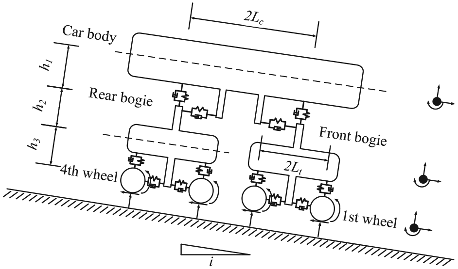
The vehicle model.
The governing equations of the car body, bogies, and wheels are derived according to the D’Alembert principle:
Bouncing vibration of car body
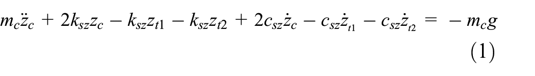
Pitching vibration of car body
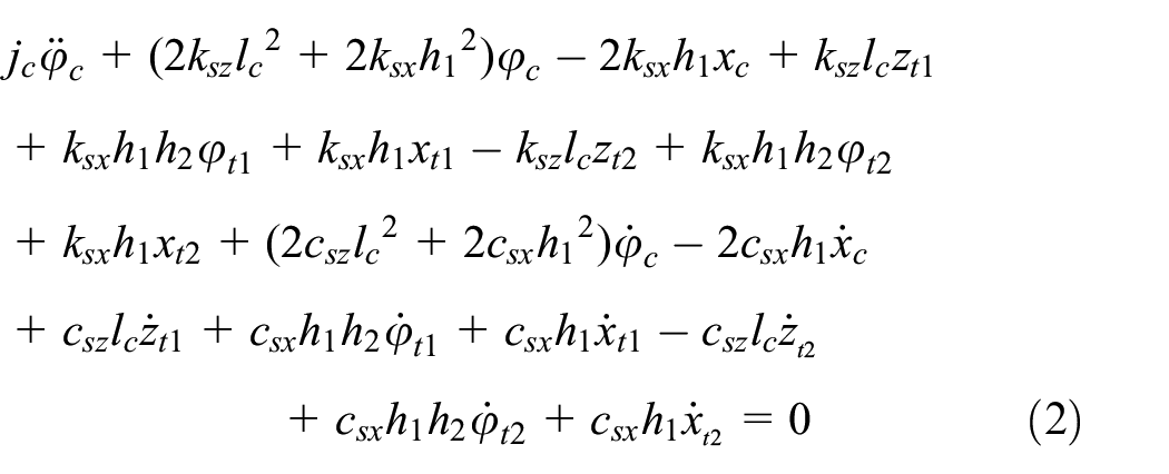
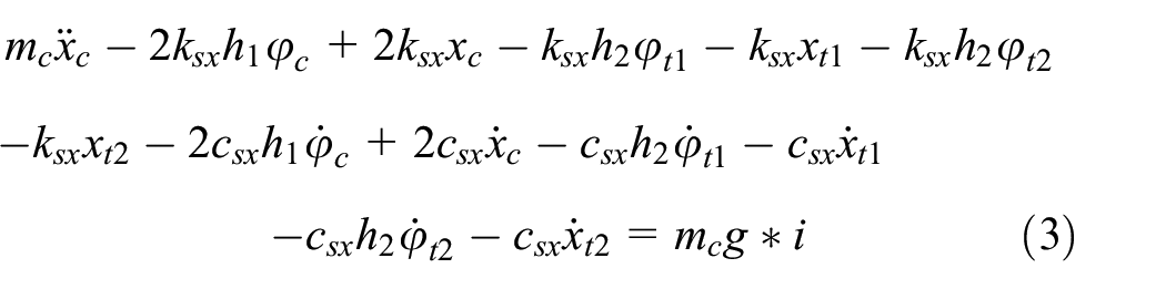
Fore-and-aft vibration of car body
Bouncing vibration of bogie

Pitching vibration of bogie
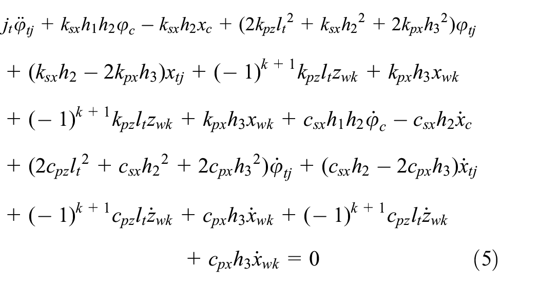
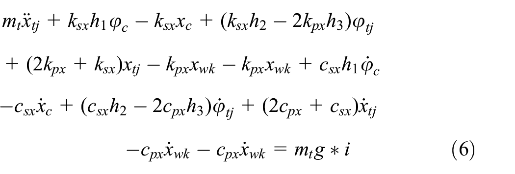
Fore-and-aft vibration of bogie
Bouncing vibration of wheel

Pitching vibration of wheel

Fore-and-aft vibration of wheel
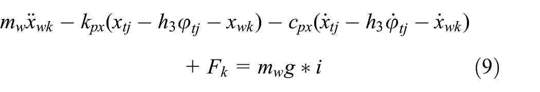
In these equations, i represents the line gradient; T represents the braking torque; mc and jc denote the mass and pitching moment of inertia of the car body, respectively; mt and jt denote the mass and pitching moment of inertia of the bogies, respectively; mw and jw denote the mass and pitching moment of inertia of the wheels, respectively; zc, φc, and xc are the vertical displacement, pitching displacement, and longitudinal position of the car body, respectively; ztj, φtj, and xtj are the vertical displacement, pitching displacement, and longitudinal position of the jth (j = 1–2) bogie, respectively; zwk, φwk, and xwk are the vertical displacement, pitching displacement, and longitudinal position of the kth (k = 1–4) wheel, respectively.
The aforementioned governing equations of the motion of vehicle are then sorted out and the dynamic equilibrium equations are established in matrix form

where Mv, Cv, Kv, and Uv represent the mass matrix, damping matrix, stiffness matrix, and displacement vector of the vehicle, respectively; Fv represents the external force vector acting on the vehicle.
“Circular track” model
In general, the foundation of high-speed railway track structure is relatively stable, so a single-layer track model is adopted. Figure 2(a) shows a finite-element model of the rail with finite length. Each node of the rail beam element has three DOFs, that is, the vertical displacement (zr), the rotation about the axis normal to the x–z plane (φr), and the longitudinal displacement (xr). The rail is supported discretely by rail pads whose elasticity and damping properties are modeled by vertically and longitudinally positioned spring–damper units.

The track model: (a) traditional track (b) circular track.
High-speed trains usually travel at such high speeds that the braking distance is about 1–2 km. If a track model is too long, the DOFs of the model will be greatly increased, and the computational efficiency will be seriously reduced. In this article, the idea of “circular track” is proposed to solve this problem.
Because the dynamic action of vehicle will only affect the response of track structure in a finite length and the effect is negligible beyond this length, it is assumed that the range of influence is (−L, L), and the origin of coordinate is the center of vehicle. In the model, the length of the track is set to be 2 L, and for mobile vehicles, the vehicle will gradually approach the front end of the track and then move away from the rear end of the track, so the range of influence will exceed the length of track in the model. In order to make the running vehicle stay at the center of track and not reach the boundary ends and also make the track responses at both ends be identical, a joint element is used to connect the two ends of the track, thus forming a “circular track” model, as shown in Figure 2(b). The “ring” in the figure is not a real ring, which is just used to illustrate that the vehicle is running at the center of the track all the time, and the responses of the track at both ends are identical.
The dynamic equilibrium equations of the “circular track” model are assembled with the direct-stiffness method, and the DOFs of the track at both ends are constrained by a joint element. The details are as follows
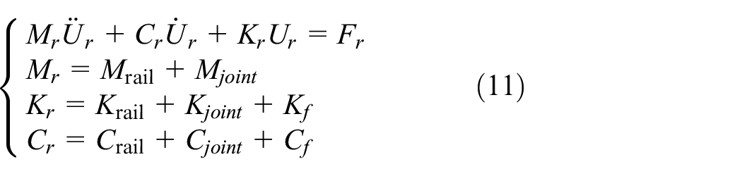
where Kr, Mr, and Cr denote the whole stiffness matrix, mass matrix, and damping matrix of the track model, respectively; Krail, Mrail, and Crail denote the overall stiffness matrix, mass matrix, and damping matrix of the rail layer, respectively; Kjoint, Mjoint, and Cjoint denote the stiffness matrix, mass matrix, and damping matrix of joint element, respectively; the stiffness matrix and damping matrix of the support layer are Kf and Cf, respectively.
The overall matrixes of the rail layer are formed by assembling all the sub-matrixes

where the stiffness sub-matrix and mass sub-matrix of the rail are as follows
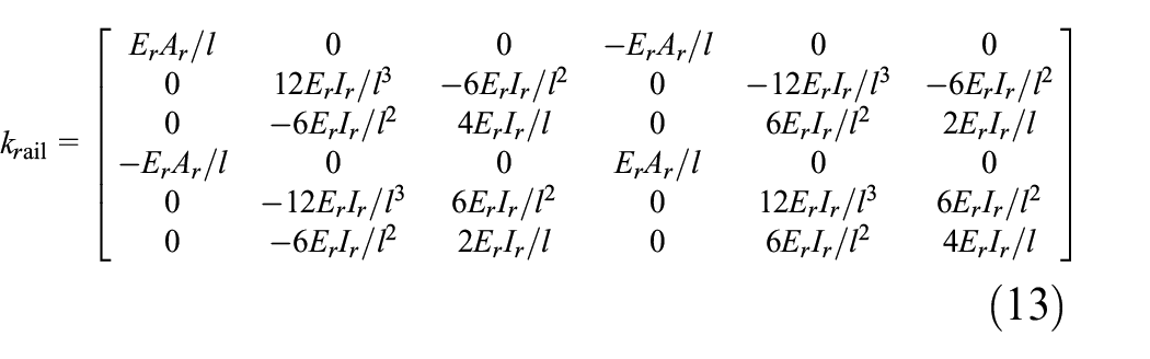
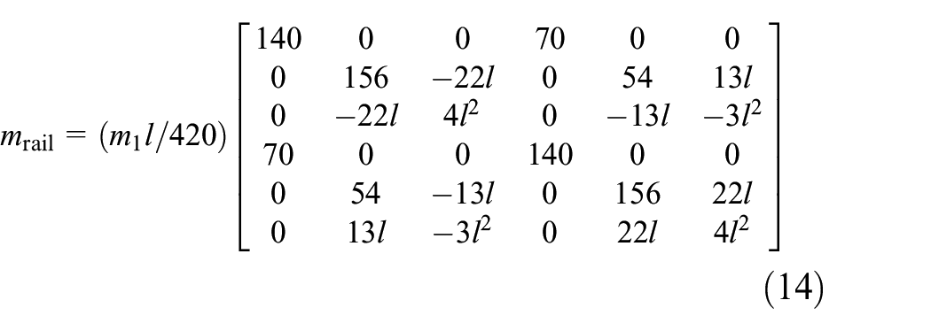
where l is the length of the rail beam element, m1 is the mass of the rail per unit length, Er is Young’s modulus of the rail, Ir is the second moment of inertia of the rail, and Ar is the cross-sectional area of the rail.
The Rayleigh damping is applied to define the damping sub-matrix

where αr and βr denote the Rayleigh damping coefficients.
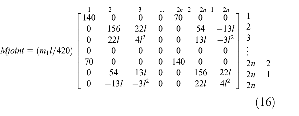
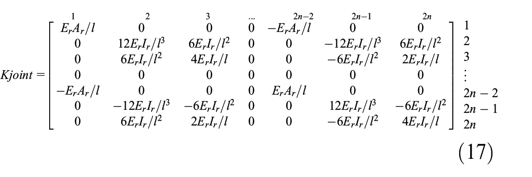
The mass matrix, stiffness matrix, and damping matrix of joint element are as follows

Similarly, the overall matrixes of the support layer are formed by assembling all sub-matrixes
Wheel–rail relationship
The wheel–rail relationship is the link between vehicle and track, so it is also the key to discover the mechanism of wheel–rail interaction. In the vehicle–track model constructed in this article, longitudinal and vertical interactions are considered, which involve the wheel–rail relationship in two directions.
Vertical wheel–rail relationship
The Hertz nonlinear contact model (Zhai and Sun, 1994) is the most classical and effective model for describing the vertical wheel–rail force, so it is used to determine the wheel–rail contact force in this article


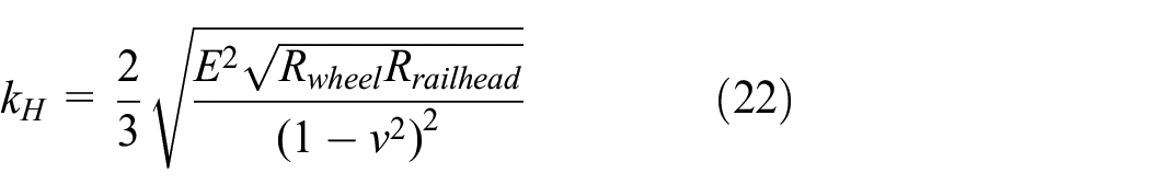
where Pk is the kth vertical wheel–rail contact force, zwk is the vertical displacement of the kth wheel, zrk is the rail displacement at the kth wheel load point, rk is the track irregularity at the kth wheel load point, kH is the Hertz contact constant, the value of coefficient Rwheel and Rrailhead denoting the radius of wheel and railhead are 0.46 m and 0.30 m, respectively, and v is Poisson’s ratio of the material with the value of 0.3.
Longitudinal wheel–rail relationship
Generally speaking, there are two kinds of methods for describing the longitudinal wheel–rail relationship: one is based on the wheel–rail creep contact theory and the other is based on the wheel–rail longitudinal rigid-contact theory (Zhang et al., 2011).
Polach creep contact theory
The creep characteristics of wheel–rail contact directly determine the braking performance and affect the running safety of a vehicle. Many scholars (Kalker, 1990; Spiryagin et al., 2013; Vermeulen and Johnson, 1964) have studied this issue, and the simplified algorithm based on the Kalker theory (Kalker, 1982; the corresponding numerical program is the Fastsim) is now widely used in the simulation of vehicle dynamics. However, according to Vollebregt (2014), in this algorithm, the Coulomb friction model with a constant friction coefficient is used, so the creep force–creepage characteristic calculated by the Kalker theory does not agree well with the measured results. Moreover, the Kalker theory cannot describe the negative slope characteristic of the adhesion curve, so its applicability is poor for the simulation of large wheel–rail creep resulting from vehicle braking.
The Polach theory (Polach, 2005) introduced reduction factors together with a slip-velocity-dependent friction coefficient, which decreases with the increase in longitudinal creepage, so the results are more accurate and the calculation is more efficient than the Fastsim. Hence, it is more reasonable to simulate vehicle braking using the Polach theory. Based on the Polach creep contact theory, the longitudinal wheel–rail force under large creep condition can be calculated rapidly as follows

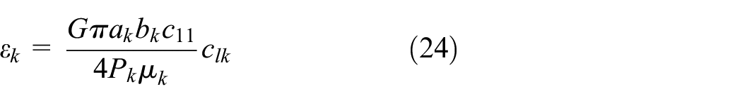
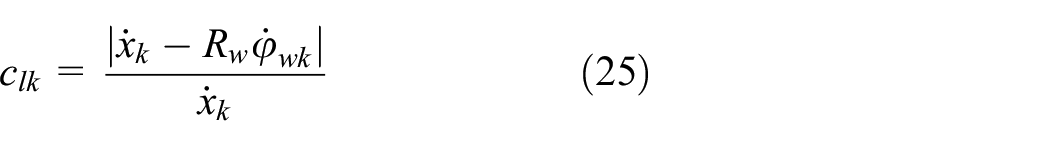
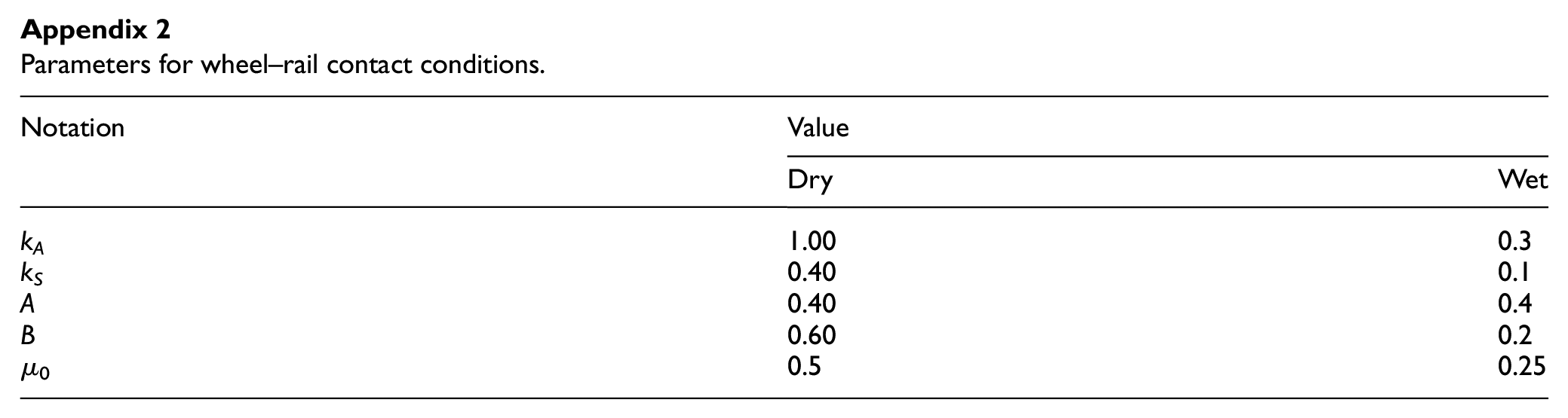
where Fk represents the kth longitudinal wheel–rail force; Pk represents the kth vertical wheel–rail contact force; εk is the gradient of tangential stress in the longitudinal direction; kA and kS are the reduction factors in the adhesion and slip areas, respectively; G is the shear modulus of rigidity; ak and bk are the semi-axes of the contact ellipse at the kth wheel with the constant value of 6 × 10⁻³ m; c11 is the Kalker coefficient with the value of 4.12; clk is the longitudinal creepage of the kth wheel; and μk is the frictional coefficient between the kth wheel and rail and can be described by

In the above equation, A is the ratio of the limit friction coefficient (μ∞) at infinite slip velocity to the maximum frictional coefficient (μ0) at zero slip velocity, and B is the coefficient of the exponential attenuation of friction; constants A and B are acquired by experiment.
2. Longitudinal rigid-contact theory
The longitudinal rigid-contact theory assumes that the longitudinal displacements of wheel and rail are equal at the contact point, that is, the longitudinal DOF of wheel is not independent; in addition, the DOFs associated with the pitching movement of wheels can also be ignored because the pitching movement and the longitudinal movement of wheels are coupled to each other. According to the assumption of longitudinal rigid contact, the longitudinal wheel–rail force acting on the track can be calculated as follows

where Fk denotes the kth longitudinal wheel–rail force acting on the track;
According to the longitudinal rigid-contact theory, the longitudinal response of the wheels can be directly imported into the vehicle and track subsystem as known data.
Solving method
Based on the wheel–rail relationships mentioned above, the kinetic equations of the vehicle subsystem and the track subsystem are sorted out, and then with the Newmark-β numerical integration method, the dynamic responses of the vehicle and track are calculated through iteration between the vehicle and track subsystem at each time step. The convergence of iteration requires that the differences between the vertical wheel–rail contact forces at adjacent steps are less than 100 N. Moreover, α and β are 0.25 and 0.5, respectively; the integration step is 0.0002 s. The procedure of computation is shown in the following chart (Figure 3).

The flow chart of calculation procedure.
Comparison of different longitudinal wheel–rail interaction models
According to the survey data, the actual speed of a China Railway High-speed (CRH) vehicle running in graded areas is in the range of 180–200 km/h. The case investigated in this section is a vehicle traveling at the initial speed of 185 km/h (51.3 m/s), which is decelerated uniformly at a deceleration of 2.55 m/s2 resulting from emergency braking. This case is simulated by two different models: the Polach creep model and the longitudinal rigid-contact model, and the parameters of the vehicle and track are shown in Appendix 1.
Figure 4 presents the dynamic responses of the vehicle and track during the braking process. The vehicle responses calculated by the two models agree well with each other in trend of variation and values, except for slight differences at the beginning and end of braking. The creep between wheel and rail is considered in the Polach model. The result shows that in the initial phase of braking, the longitudinal wheel–rail creepage increases gradually, the sliding area expands gradually, and the longitudinal wheel–rail force increases gradually, so the time history of vehicle response is flatter; at the end of braking, the large creep caused by vehicle impact leads to the occurrence of wheel sliding, and the frictional coefficient becomes lager with the decrease in speed, so the longitudinal wheel–rail force increases suddenly. In contrast, the creep between wheel and rail is not considered in the longitudinal rigid–contact model. The result shows that in the initial phase of braking, the braking force is suddenly applied; at the end of braking, the braking force is immediately withdrawn, so significant fluctuation is observed in the response of vehicle at the beginning and end of braking. However, the dynamic responses of track calculated by the two models accord quiet well with each other.
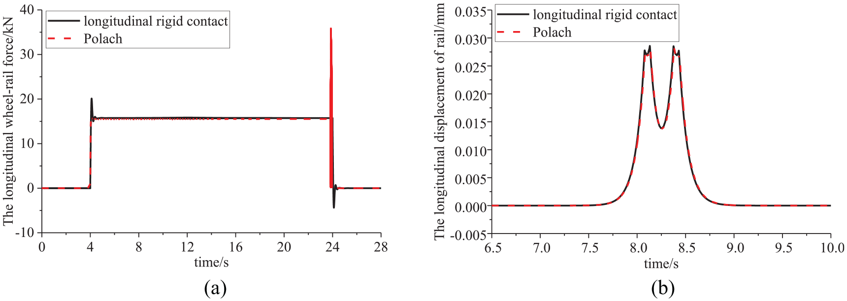
Comparison of the two models: (a) the time history of longitudinal wheel–rail force and (b) the time history of longitudinal displacement of rail.
Comparison of the dynamic responses of vehicle and track calculated by the two models suggests that when studying the dynamic response of track and bridge structure under the condition of vehicle braking, the longitudinal rigid-contact model can be used as a fast and effective simulation model. However, it is hard to reflect the wheel–rail interaction mechanism, and it can neither describe the movement characteristics of wheels in the braking process and the creep characteristics between wheel and rail nor be used to study the damage of wheel–rail interface.
Braking under different operational conditions
In this section, the Polach creep model is used to simulate the braking process and the effects of braking torque, line gradient, and rail-surface irregularity are investigated on the dynamic responses of vehicle and track. The parameters of the simulated vehicle and track are shown in Appendix 1.
Braking torque
Under some unexpected situations, vehicles often need to decelerate and halt when running on a grade. Usually, depending on the actual situation, various braking levels may be applied; more specifically, various braking torques may be applied to the wheels to halt the vehicle. In order to simulate various braking levels, the braking torque is set to be 3, 5, 7, 8, 9, 10.5, 11, and 13 kN m alternately. The initial braking speed of the vehicle is set to be 185 km/h (51.3 m/s), and the gradient of grade is set to be 5‰.
Figure 5 lists the time history of the motion of each wheel when various braking torques are applied. Based on the difference between the angular speed of wheels and the speed of vehicle, the braking torques can be roughly divided into five intervals: 0–8 kN m, 8–9 kN m, 9–10.5 kN m, 10.5–11 kN m, and 11–13 kN m). When the braking torque increases gradually from 0 to 8 kN m (as shown in Figure 5(a), the angular speed of wheel and the speed of vehicle decrease proportionally; in this stage, the wheels remain at the rolling state, and the wheel–rail rolling friction forces are used to resist the traveling of vehicle. When the torque continues to increase in the range of 8–9 kN m (as shown in Figure 5(b)), the angular speed of the fourth wheel is reduced to zero quickly owing to the resistance provided by the torque; however, at this time, the speed of vehicle is not zero, so the fourth wheel no longer roll, and begin to be locked and slide until the halt of vehicle. This wheel sliding will cause damage to the wheel–rail interface, which will induce abnormal wheel–rail impact force and exacerbate the fatigue failure of the vehicle–track structure. When the braking torque is increased further to the range of 9–10.5 kN m, 10.5–11 kN m, and 11–13 kN m (as shown in Figure 5(c) to (e), respectively), the second pair of wheels, the third pair of wheels, and the first pair of wheels will successively change from the rolling state to the sliding state.

Time history of wheel angular speed and vehicle speed under various braking torques: (a) 7 kN m, (b) 8 kN m, (c) 9 kN m, (d) 10.5 kN m, and (e) 11 kN m.
Figure 6 presents the time history of longitudinal deceleration of vehicle when braking torques with various levels are applied. When the braking torque is 7 kN m (Figure 6(a)), the wheels have been rolling during the braking process, and the longitudinal wheel–rail forces keep basically stable; however, the longitudinal wheel–rail force is directly related to the longitudinal response of vehicle, so the longitudinal deceleration of vehicle is basically unchanged. When the braking torque is 13 kN m (Figure 6(b)), the motion of wheels will change during the braking process, leading to the variation in longitudinal wheel–rail force, which will then affect the longitudinal deceleration of vehicle, so the longitudinal deceleration can be divided into three stages based on the motion of wheels: the creep stage, sliding stage, and low-speed sliding stage. In the creep stage, with the progress of braking, the wheel–rail creepage increases gradually, the longitudinal wheel–rail force decreases correspondingly, and the deceleration of vehicle decreases gradually. In the sliding stage, the frictional coefficient is less affected by the speed of vehicle, and the sliding friction force remains stable, so the deceleration of vehicle keeps basically stable. In the low-speed sliding stage, the frictional coefficient increases gradually with the decrease in sliding speed, and the longitudinal wheel–rail force increases accordingly, leading to gradual increase in the deceleration of vehicle.

Time history of the longitudinal deceleration of vehicle under various braking torques: (a) 7 kN m and (b) 13 kN m.
Figure 7 presents the variations of braking distance and braking time of the vehicle with the level of braking torque. When the braking torque is small, all the wheels creep, and the braking distance and braking time decrease noticeably with the increase of the torque. When the torque is greater than 8 kN m, wheel sliding occurs; with the increase of torque, the decline of braking distance and braking time is not salient and it is noted that any further increase in the torque does not result in any decrease in the braking distance and braking time, but will cause the damage of wheel–rail interface. To ensure the safety of vehicle operation, the braking distance and braking time should be shortened as much as possible under the premise that the wheels will not be locked or slide along the surface of rail. Based on the results calculated in this section, it is quite reasonable to set the level of braking torque to be 7 kN m.
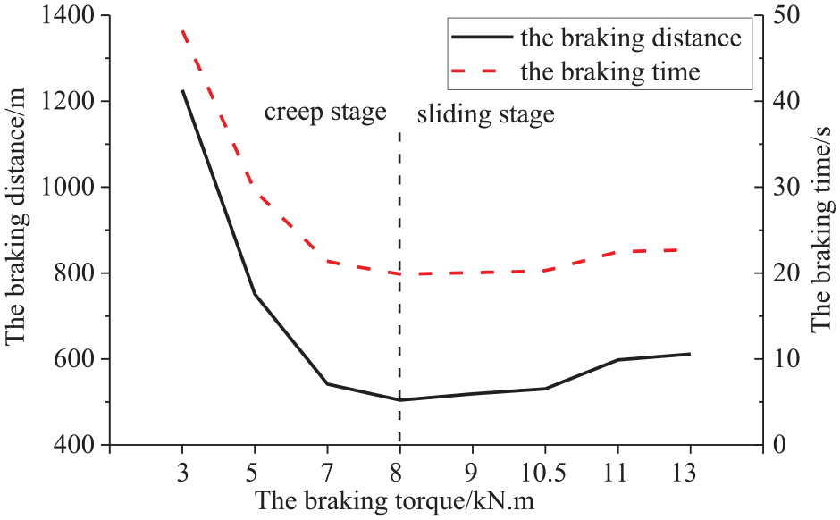
The braking distance and time under various braking torques.
It is well known that the friction coefficient of the wheel–rail interface has a great influence on the longitudinal creepage; in order to further study the influence of the braking torque on the vehicle response under different friction coefficients, the case of a train traveling on the dry/wet track before experiencing sudden deceleration due to the application of braking torques is considered. Wheel–rail contact parameters are shown in Appendix 2. Figure 8 presents the variations of sliding time and braking distance of the vehicle with the level of braking torque under both wet track and dry track conditions; it can be seen that when the braking torque is less than 5 kN m, there is no occurrence of wheel sliding under two kinds of wheel–rail contact conditions; in this stage, the braking distance of the vehicle is also equal. When the torque increases to 5 kN m, here are occurrences of wheel sliding under wet track condition; at this time, the braking distance is minimized. When the torque reaches 8 kN m, the wheel begins to slide under dry track condition and the braking distance is minimized. On the whole, under wet track condition, the friction coefficient of the wheel–rail interface is smaller and the maximum longitudinal wheel–rail force is smaller correspondingly; therefore, it is easier for the wheel to slide; however, the sliding time and the braking distance are longer.
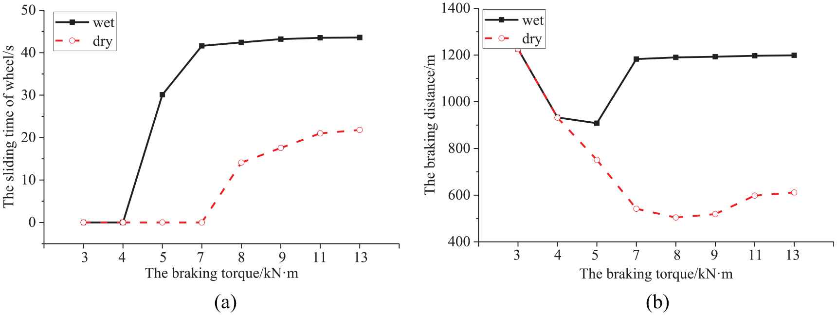
The responses of vehicle under various braking torque under dry/wet track condition: (a) the sliding time (b) the braking distance.
Gradient
The maximum gradients of high-speed railway lines are generally 20‰–40‰. In order to analyze the effects of different line conditions on the braking of vehicle, a grade with gradient of 40‰ is set in the braking path of the vehicle. The initial braking speed of the vehicle is set to be 185 km/h (51.3 m/s), and the braking torque is set to be 7 kN m.
Figure 9 presents the time history of the longitudinal deceleration of the vehicle, longitudinal wheel–rail force, and longitudinal creepage in the braking process. The longitudinal deceleration of the vehicle remains stable on the flat track; however, when the vehicle travels to the grade, the longitudinal deceleration suddenly decreases owing to increased load along the line direction. The sudden change in the longitudinal deceleration of the vehicle on the grade leads to sudden change in the longitudinal velocity of the wheels, resulting in sudden change in the longitudinal creepage of the wheels at the point of gradient jump. The longitudinal wheel–rail force also changes correspondingly. It should be noted that the damage of wheel–rail interface is more likely to happen with the increase in longitudinal creepage.
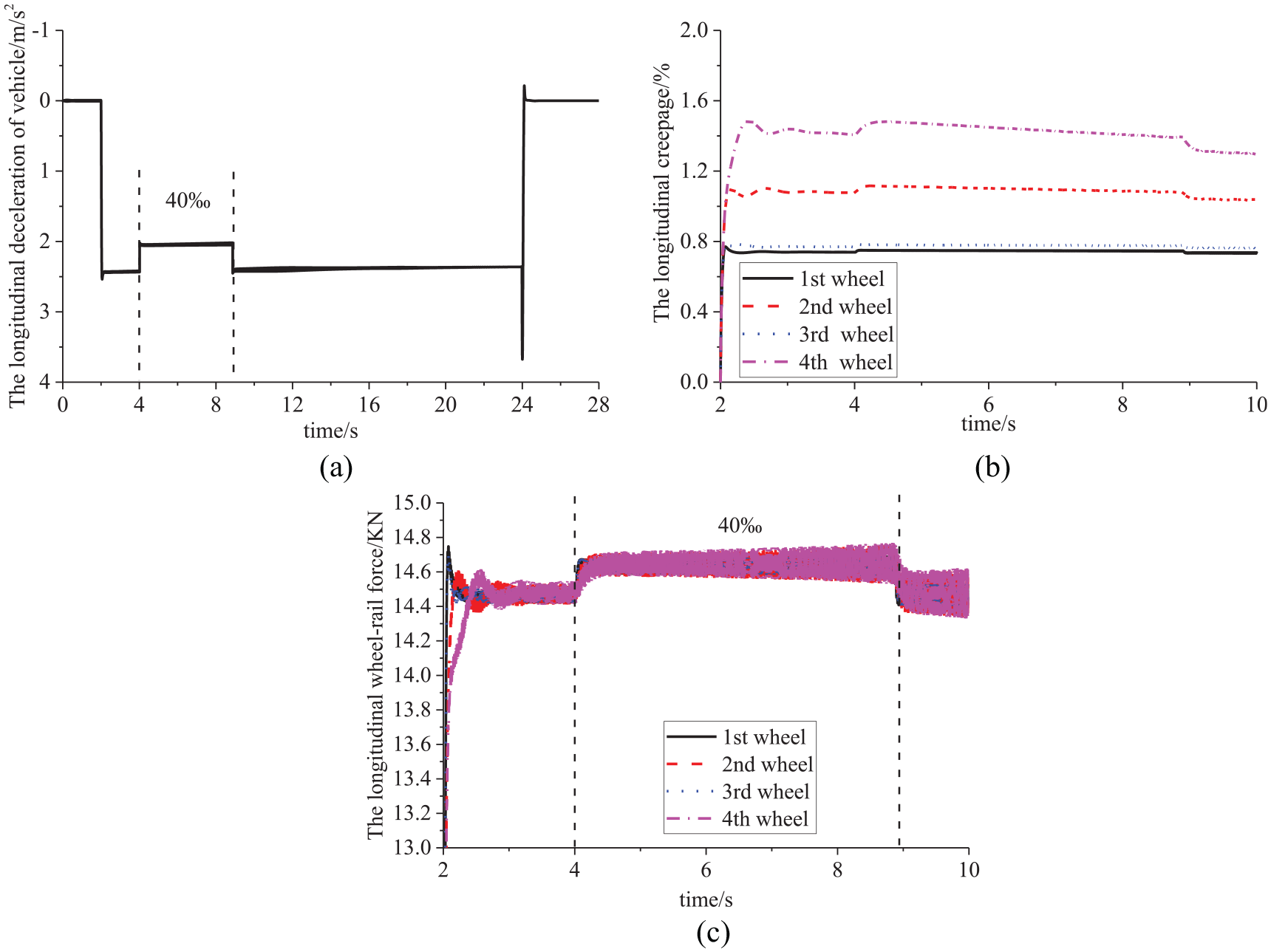
(a) The time history of longitudinal deceleration of vehicle, (b) the time history of longitudinal wheel–rail creepage, and (c) the time history of longitudinal wheel–rail force.
Next, a long enough grade with gradient of 0, 10‰, 20‰, 30‰, and 40‰ is set up alternately to investigate the effect of gradient on vehicle braking in more depth. The vehicle is decelerated at various braking levels on the grade.
In view of the fact that the motions of the four wheels are similar during the process of vehicle braking (although the fourth wheel begins to slide first with the increase in torque), Figure 10 only shows the sliding time of the fourth wheel under various gradients when braking torques with different levels are applied. Figure 10 also shows that under various gradient conditions, the maximum braking torque without wheel sliding is 7 kN m, which is consistent with the result obtained in section “Comparison of different longitudinal wheel–rail interaction model.” Hence, it can be concluded that gradient will not alter the reasonable level of braking torque. However, when the wheel begins to slide, the sliding time increases gradually with the increase in gradient, suggesting that the risk of wheel–rail interface damage is greater when the vehicle brake is on a grade.
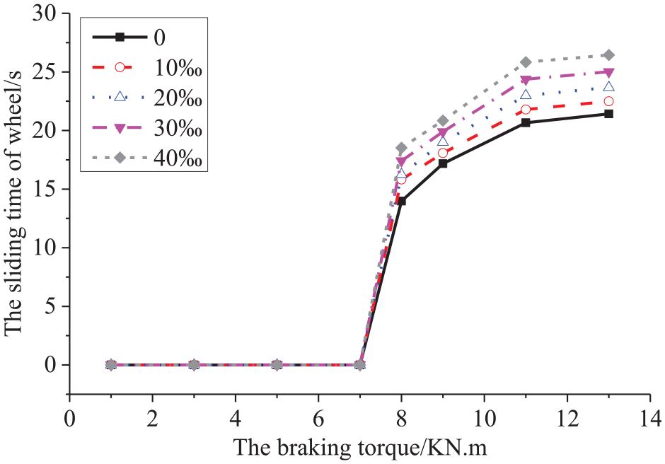
The wheel sliding time under various gradient and torque conditions.
Figure 11 shows the longitudinal deceleration, braking distance, and braking time of the vehicle on a grade with various gradients, when the wheels are subject to the braking torque of 7 kN m. With the increase in gradient, the load along the line direction gradually becomes larger and the longitudinal deceleration of the vehicle decreases gradually. The decrease in longitudinal deceleration leads to significantly increased braking distance and braking time (541 m and 21.3 s on the flat track, respectively; 642 m and 25.4 s on the grade with gradient of 40‰, respectively). It can be concluded that braking on the grade is disadvantageous; in order to ensure the safety of vehicle operation, it is necessary to limit the running speed of vehicle on the grade.

(a) The longitudinal deceleration of vehicle under various gradient and (b) the braking distance and time under various gradient.
Random irregularity
The rail surface cannot be smooth in an actual situation, and random irregularity is present owing to the combined effects of many factors such as initial bending, wear, and damage of track. In order to study the effect of random irregularity on the dynamic interaction between wheel and track under braking conditions, superimposition of short-wave irregularity over medium-long-wave irregularity is adopted to simulate the actual track irregularity. The initial braking speed of the vehicle is set to be 185 km/h (51.3 m/s), and the gradient of the grade is set to be 5‰.
Figure 12 shows the vertical wheel–rail force of the first and fourth wheels at two states: on a smooth track and on a track with irregularity. When the braking torque is applied, the body and bogies pitch downward and axle-load transfer occur, so the vertical wheel–rail force of the first wheel increases significantly and the vertical wheel–rail force of the fourth wheel decreases significantly. In the presence of irregularity, high-frequency fluctuation is found in the vertical wheel–rail force; the rail surface in contact with the wheels is prone to fatigue damage under repeated actions of high-frequency force, reducing the maintenance cycle and service span of the track. In addition, the short-wave component of irregularity causes transient impact vibration of the wheel–rail system, resulting in a sudden three to four times of increase in the wheel–rail contact force and impact damage to wheel–rail system.
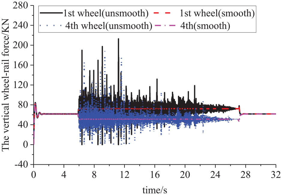
The time history of vertical wheel–rail force.
Figure 13(a) and (b) presents the time history of longitudinal wheel–rail force and longitudinal deceleration of the vehicle, respectively. Under the influence of vertical wheel–rail force, violent oscillation is observed in the longitudinal wheel–rail force in the presence of irregularity, mostly likely leading to uneven deformation of rail surface and then wave corrugation. Moreover, vehicle braking is achieved through the generation of longitudinal wheel–rail force at the wheel–rail interface, so the fluctuation of longitudinal deceleration is similar to that of the longitudinal wheel–rail force; during braking, the fluctuation is gradually weakened with the decrease in the speed and does not disappear until the halt of vehicle.
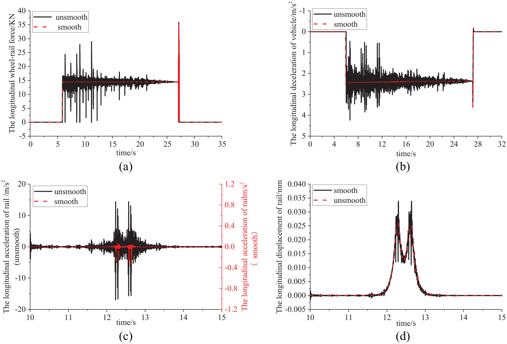
The time history of longitudinal response of vehicle and track: (a) longitudinal wheel–rail force, (b) the longitudinal deceleration of vehicle, (c) the longitudinal acceleration of rail, and (d) the longitudinal displacement of rail.
Figure 13(c) and (d) shows the time history of the longitudinal deceleration and displacement of the track at the two states. The response of track reach peaks at the points of wheel load and the short-wave component of track irregularity cause the longitudinal wheel–rail force to oscillate violently, greatly exacerbating the longitudinal vibration of track structure. When the track is smooth, the peaks of the longitudinal acceleration and longitudinal displacement of track are 0.3 m/s2 and 0.026 mm, respectively, while the peaks of the longitudinal acceleration and longitudinal displacement of track are 18 m/s2 and 0.033 mm, respectively, in the presence of track irregularity.
Flexible track versus rigid track
In order to analyze the influence of track vibration on the wheel–rail dynamic response under braking conditions, the rigid track model and the flexible track model are established, respectively, to investigate the wheel–rail force under the action of braking torque (7 kN m). The initial braking speed is 185 km/h (51.3 m/s), and the track irregularities mentioned in section “Random irregularity” are used.
Figure 14(a) and (b) shows the time-history and frequency spectrum of the vertical wheel–rail force obtained by two models: flexible track and rigid track. It can be seen that due to the excitation of random track irregularities, the fluctuation of the vertical wheel–rail force calculated by the flexible track is obviously lower than that of the rigid track and mainly reflects in the high frequency, which is due to the attenuation of the wheel–rail force by the elasticity/damping of the track structure. In the spectrum, it is not difficult to find that the vertical wheel–rail force calculated by flexible and rigid track is basically the same when the frequency is lower than 30 Hz. In the frequency range of 30–50 Hz, the vertical wheel–rail force of the former is slightly higher than that of the latter. For the high-frequency range exceeding 50 Hz, the vertical wheel–rail force when the track is flexible is significantly lower than that when the track is rigid.
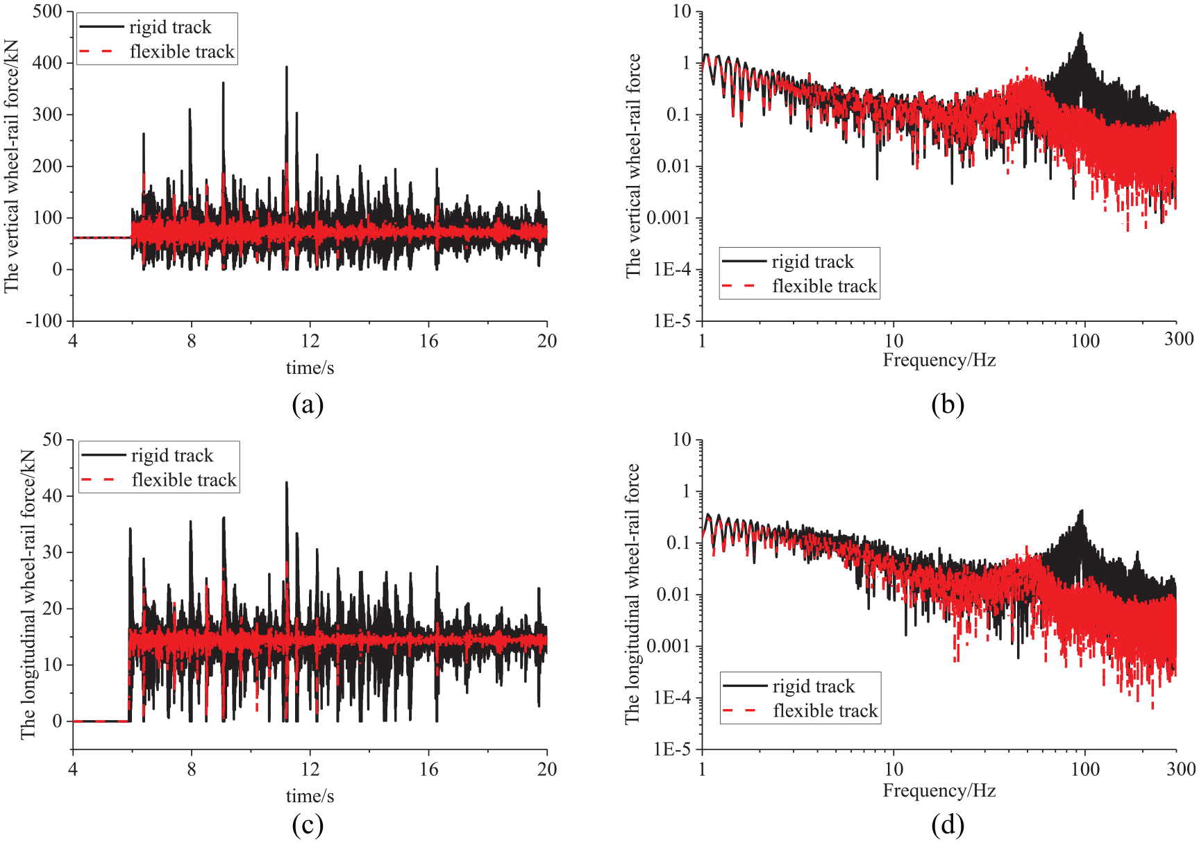
(a) Time history of the vertical wheel–rail force, (b) frequency spectrum of the vertical wheel–rail force, (c) time history of the longitudinal wheel–rail force, and (d) frequency spectrum of the longitudinal wheel–rail force.
Figure 14(c) and (d) shows the time history and frequency spectrum of the longitudinal wheel–rail force. Similarly, in the presence of the random irregularity, due to the attenuation effect of track structure on vibration, the fluctuation of the longitudinal wheel–rail force of flexible track is also lower than that of the rigid track. The discrepancy of longitudinal wheel–rail force calculated by two models mainly reflected in the high frequency.
Conclusion
In this article, a vehicle–track interaction model on a grade is constructed based on two longitudinal wheel–rail interaction models (the Polach creep model and the longitudinal rigid-contact model), and the dynamic responses of vehicle and track caused by vehicle braking on the grade is studied. The following conclusions are obtained:
When the Polach creep model and the longitudinal rigid-contact model are used as the longitudinal wheel–rail interaction model, the calculated dynamic responses of substructure show little difference. However, the Polach creep model can fully consider the motion of wheels and large wheel–rail creep phenomenon in the braking process and can accurately analyze the damage of wheel–rail interface.
Large braking torque will cause some or all of the wheels to slide and then trigger the damage of wheel–rail interface. The grade will lead to the increase in braking distance and time and extend the sliding time of locked wheel, increasing the risk of damage at the wheel–rail interface.
In order to ensure the safety of running, the braking torque should be kept below a reasonable value, so the braking distance and time could be shortened as far as possible without the occurrence of sliding wheel. According to the calculation in this article, the braking torque under the dry track and wet track conditions should be 7 and 4 kN m, respectively.
In the process of vehicle braking, the car body and bogie pitch downward, causing increased load at the front wheel and reduced load at the rear wheel. The irregularity of rail surface exacerbates high-frequency fluctuation of the vertical and longitudinal wheel–rail contact forces, mostly likely leading to the fatigue damage of wheel–rail and the corrugation of rail.
Since the flexible track structure has elasticity and damping effect, the vertical wheel–rail force, especially the high-frequency component, can be effectively buffered and attenuated, and the longitudinal wheel–rail force will also be moderated. Thus, the elasticity of the track structure can improve running stability of the vehicle under the action of braking torque.
Footnotes
Appendix
Parameters for wheel–rail contact conditions.
| Notation | Value |
|
|---|---|---|
| Dry | Wet | |
| kA | 1.00 | 0.3 |
| kS | 0.40 | 0.1 |
| A | 0.40 | 0.4 |
| B | 0.60 | 0.2 |
| μ 0 | 0.5 | 0.25 |
Declaration of Conflicting Interests
The author(s) declared no potential conflicts of interest with respect to the research, authorship, and/or publication of this article.
Funding
The author(s) disclosed receipt of the following financial support for the research, authorship, and/or publication of this article: The research is sponsored by Beijing Municipal Natural Science Foundation (Grant No. 8182041) and the National Natural Science Foundation of China (Grant No. 51578054).