
Abstract
Previous research showed that wind characteristics were influenced by terrain. To accurately calculate the wind-induced bridge response, this article presented a comprehensive investigation of the wind characteristics of a trumpet-shaped mountain pass by long-term monitoring. Basic strong wind characteristics such as the wind rose, turbulence intensities, turbulence length scales, turbulence spectra and normalized cross-spectrum were discussed using 10 min intervals. Due to the different types of terrain on the two sides of the bridge site, this article attempted to reflect the influence of the terrain on the wind characteristics in different wind directions. The scatter plots of wind characteristics were presented directly on the terrain map. The effects of the turbulence characteristics, mean wind speed and aerodynamic admittance function on buffeting response of the composite cable-stayed bridge were discussed by the multimode coupled frequency domain. The results show that the wind profile is extremely twisted. The larger turbulent integral scale and the lower turbulence intensity appear in the direction along the river. The effect of the mean wind speed on the buffeting response is greater than that of the fluctuating wind characteristics. The aerodynamic admittance function proposed by Holmes has the largest reduction in buffeting response.
Keywords
Introduction
A flexible structure is sensitive to wind loads. Based on the random vibration theory, the key to accurately calculating the buffeting response of a bridge is the correct understanding of the wind field characteristics at the bridge site and the aerodynamic admittance function (Davenport, 1961a; Ma et al., 2019b). Many scholars have studied wind characteristics based on experience, semi-empirical and theoretical methods that are used to guide structural wind resistant design (Solari and Piccardo, 2001). However, wind characteristics in complex terrains and homogeneous terrains have an obvious difference (Li et al., 2017), and whether this difference will affect the bridge structure during the construction and operation states is very important. With respect to the wind characteristics of complex terrains, field measurements are critical to obtain the accurate wind characteristics. Hui et al. (2009a, 2009b) studied the wind field characteristics by the mast at the Stonecutters Bridge site. Øiseth et al. (2013) fitted the vertical and horizontal turbulence co-spectral densities of the Sotra Bridge and studied the influence of the cross-spectrum on the buffeting response. The results showed that the cross-spectrum density has little effect on the buffeting response compared to the uncertainty of the wind field. Recently, there have been a great number of studies in the literature performed on the long-term monitoring wind field and analysed the influence of the terrain on the wind characteristics (Hu et al., 2013; Tao et al., 2016; Wang et al., 2016). Unfortunately, field measurements have mainly been focused on gorge terrains, mountainous terrains or fjords and have rarely been aimed at the mountain pass. Moreover, based on the measured wind characteristics, the Π-shaped girder cable-stayed bridge buffeting research has been rarely reported. The composite Π-shaped girder is easy to assemble. Therefore, it is a popular choice, for example, the Yangpu Bridge (Gu et al., 1999) and Qingzhou Min River Bridge (Ren et al., 2007). However, compared with concrete cable-stayed bridges, the composite cable-stayed bridge is small in mass and has a low girder torsional rigidity. Therefore, the bridge is more sensitive to wind load (Zhou et al., 2015).
The buffeting response prediction includes time domain method and frequency domain method (Chen et al., 2000; Davenport, 1962). The structural nonlinearity and aerodynamic nonlinearity can be considered in time domain method, but the computational efficiency and programme generality are poor. Generally, the frequency domain method is restricted to linear analysis, but the computational efficiency is high. Simultaneously, the aerodynamic admittance function expressed in frequency domain can be conveniently considered. The aerodynamic admittance function is the transformation function of the turbulent wind velocity and the buffeting force. William R Sears derived the aerodynamic admittance function of an airfoil. However, it is difficult to obtain a theoretical solution of the aerodynamic admittance function for a bluff body. Zhu et al. (2018) identified the six-component aerodynamic admittance of the closed-box bridge deck in a wind tunnel test. Ma et al. (2019a) studied the aerodynamic characteristics of the bridge girder and buffeting response through field measurements. To date, few studies have measured the aerodynamic admittance function of a Π-shaped girder.
This article analyses the wind characteristics of a trumpet-shaped mountain pass. According to the difference in the terrain on the two sides of the bridge, this article attempts to reflect the effects of the terrain on the wind characteristics in different directions. Based on the designed wind characteristics and measured wind characteristics, the buffeting response of the Π-shaped girder is calculated using the multimode coupled frequency domain method. To analyse the influence of the aerodynamic admittance function on the buffeting response, the buffeting response is calculated by using different aerodynamic admittance functions from the literature (Davenport, 1962; Holmes, 1975; Liepmann, 1952).
Bridge and monitoring system
The Longmen Bridge is a composite cable-stayed bridge. The main girder is the Π-section with an overall length of 680 m (52 m+113m+350m+113m+ 52 m), as shown in Figure 1. The total width of the girder is 38.5 m with two-way six lanes. There are 112 stay cables in total. The stay cable consists of 109 (Ø7 mm) galvanized steel wires. The design speed is 80 km/h.

Configuration of the Longmen bridge (cm).
The bridge site is a trumpet-shaped mountain pass on the Loess Plateau. This terrain has the following three characteristics: (1) The bridge is at the junction of the mountains and valleys. The terrain on both sides is completely different. (2) The mountains affect the wind direction and generate a backflow or wake at the bridge site. (3) The terrain at the bridge site is a trumpet-shaped mountain pass, which has an expanding effect on the northwest wind and a compression effect on the southeast wind. To date, there have been few observations about the wind characteristics of this type of terrain.
To observe the wind characteristics of the bridge site, three masts are built at the bridge site. M1 is a 60 m high mast on the right bank of the river, and M2 and M3 are 30 m high masts located on the northeast and southeast sides of the west approach bridge, respectively. A three-dimensional (3D) anemometer (CSI CSAT3) is installed on the top of each three masts. The 60 m high mast has a two-dimensional (2D) ultrasonic anemometer (2D Gill WindSonic) at 10, 20 and 45 m heights, and two 2D anemometers are mounted on the platform at a height of 30 m with a horizontal distance of 18 m. All 2D ultrasonic anemometers can simultaneously write wind data into a file and provide diagnostic values for each file. The 3D ultrasonic anemometer has a vertical measurement path of 10 cm, operates in a pulsed acoustic mode, and can withstand harsh weather conditions. Three orthogonal wind velocity components can be measured and output at a maximum frequency of 60 Hz, providing both analogue and digital signal output formats. The sampling frequency is 4 Hz for the 2D ultrasonic anemometer and 10 Hz for the 3D ultrasonic anemometer. This study selects 10 min time interval analysis data. The masts layout is shown in Figure 2, and a diagrammatic illustration of the 60 m mast is shown in Figure 3.
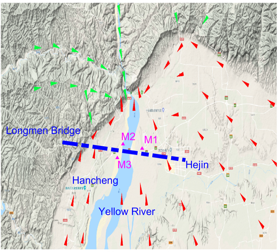
Bridge site and mast layout.
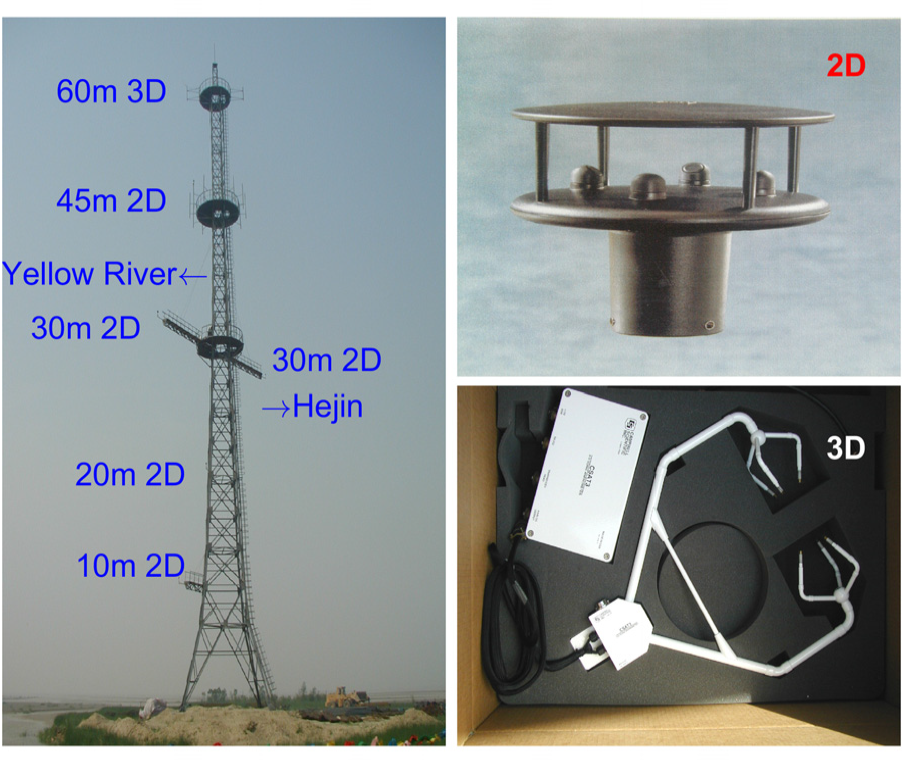
A diagrammatic illustration of the 60 m mast (M1).
Data and results analysis
Mean wind and wind profile
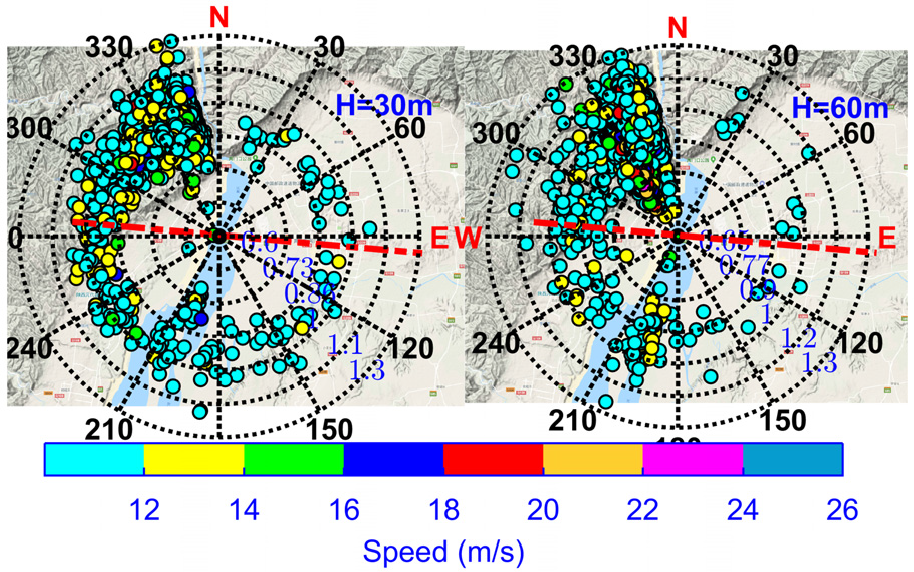
The wind data for this study cover 345 days. The erroneous data of five 2D ultrasonic anemometers are discarded. Samples with a mean wind speed of not less than 10 m/s at the same time are selected (Masters et al., 2010). Wind velocity analyses are carried out on 885 extracted samples. The wind rose is plotted on the top of the terrain map of the bridge site to show the relationship between the wind velocity and terrain. In Figure 4, the blue dotted line corresponds to the longitudinal axis of the Longmen Bridge. There is a slight difference between the 2D-Hejin and 2D-Yellow River in terms of the mean wind data. Therefore, this research selects the anemometer near the river at 30 m.
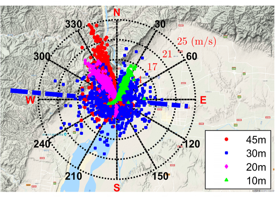
Wind speed and direction.
Figure 4 shows the wind profile under this terrain is much more twisted than that in homogeneous terrain. The wind direction at a height of 10 m is mainly concentrated near 30°, and there are a few southeast wind records. The wind direction at a height of 20 m is mainly concentrated near 330° and 180°. The wind directions at 30 m are relatively scattered. The wind direction at a height of 45 m is concentrated at 340°, and the maximum wind speed also appears at this height. Both the amplitude and number of the samples in the northwest direction are greater than the amplitude and number of the samples in other directions. Because the airflow close to the ground is more susceptible to topography, the airflow at a height of 10 m is parallel to the river, which is the lowest elevation in the bridge site. The northwest flow, 20 m in height, is blocked by the western ridge, and then divided into two different parts. Thus, the wind direction is approximately parallel to the ridge or riverbed. The airflow at the height of 30 and 45 m are affected by the mountains, airflow separation may occur and the wind direction fluctuates sharply. The airflow flows along the river valleys or mountain edges and rarely appears at 345°–15° (clockwise).
Furthermore, all strong wind data are divided into six intervals according to the wind direction at the 45 m height. The wind speed of each interval sample is averaged. Figure 5 shows the averaged wind profile for six wind direction ranges. The averaged wind profiles that approximates the power law are fitted. This figure indicates that the wind profile approximate satisfies the power law at 180°–240° and 300°–360°, which correspond to the downstream and upstream flow of the Yellow River. The index of the fitting power law is 0.0938 and 0.164, respectively. The power law is not followed within the observed height in other direction ranges because the mountain blocks the airflow, and then a windward or leeward vortex is produced.
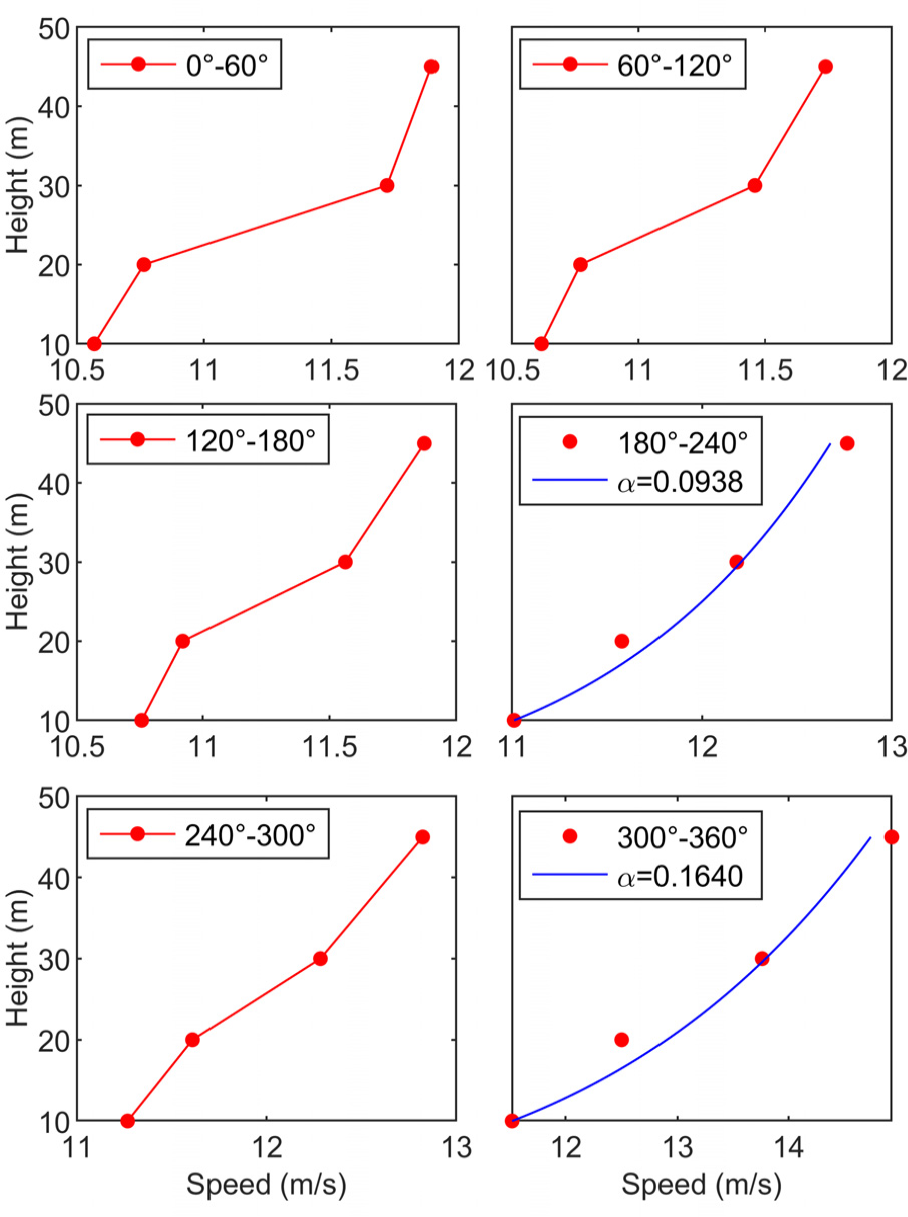
Wind profiles of the various wind direction ranges.
Roughness length
Many methods have been developed for the estimation of the roughness length, which can be categorized into three types: micrometeorological methods, classification methods and morphometric methods (He et al., 2017). The wind profile method, which belongs to the micrometeorological method, is selected to calculate the roughness length at 300°–360°. The bridge site is approximately 4 km away from the mountain, which is much larger than the mountain height. Generally, the roughness length considers the influence of the upstream topographical within 2 km, so the boundary layer adjustment is not considered (Jarraud, 2008). To test for the strong wind samples, each sample needs to meet three conditions (He et al., 2013): (1) the standard deviation of the wind direction is not greater than 15°; (2) the peak wind speed that deviates from the mean speed is less than five times the standard deviation of the speed and (3) the neutral condition can be satisfied when the 10 min mean wind speed is greater than 10 m/s.
For the neutral atmospheric boundary layer, the wind profile can be depicted as equation (1) in 300°–360°.

where
According to the mean wind data of different heights,
The roughness length is calculated by randomly selecting the wind speed at two different heights. The results are shown in Figure 6. According to the loglikelihood test, the optimal fit distribution is a Gamma distribution. The shape parameter is 1.3752 and the scale parameter is 0.2155. Figure 6 shows that the measured roughness length at the peak of the probability density is 0.121.
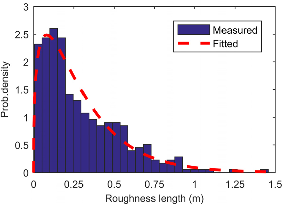
Probability density of the roughness length.
Turbulence characteristics
For the 3D wind data, the mean wind speed is computed based on the measured mean east and south wind speeds (Xu and Zhan, 2001)

Thus, the fluctuating wind speed in the longitudinal, lateral and vertical directions are calculated by

Turbulence intensity
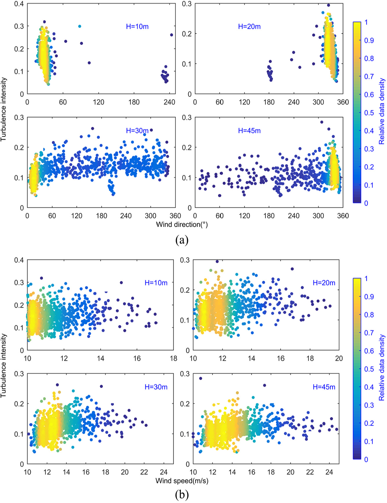
The turbulence intensity is the ratio between the standard deviation of the fluctuating wind speed and the mean speed. Figure 7 provides an overview of the longitudinal turbulence intensity characteristics.
(a) Relationship between the turbulence intensity and direction and (b) Relationship between the turbulence intensity and speed.
Figure 7 shows the strong wind direction is concentrated at 300°–30° (clockwise). The wind speed is generally in the 10–15 m/s. The lower turbulence intensity appears at 180°–240°, which corresponds to the downstream of the river. The mean turbulence intensities at 10, 20, 30 and 45 m are 0.1473, 0.1368, 0.1251 and 0.1165, respectively. The turbulence intensity at 10 m height is stable with increasing wind speed but slightly increased at 20–45 m. The data of the 3D anemometer are analysed. The scatter plots with the measured turbulent intensity are shown in Figure 8.
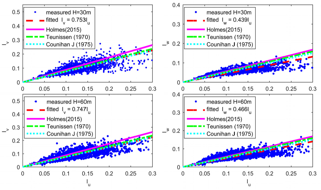
The relationship between the turbulent intensity.
The results show that the correlation between the along-wind and lateral turbulence intensities at both heights is approximately 0.75. The correlation between the horizontal and vertical turbulence intensities at 60 m height is higher than 30 m. The turbulence intensity correlation between the horizontal directions is more discrete than the correlation between the horizontal and vertical directions, which may be due to the unstable fluctuating wind speed in the lateral direction. Compared with previous studies, the correlation of the turbulence intensity between the horizontal directions is almost consistent with that of Counihan (1975), but lower than that of Teunissen (1970) and Holmes (2015). The correlation of the turbulence intensity between the horizontal and vertical directions is lower than that of Counihan (1975), Teunissen (1970) and Holmes (2015).
Turbulence length scale
If the turbulence is a stationary stochastic process and Taylor’s hypothesis of the frozen turbulence is assumed valid, then the along-wind turbulence length scales can be estimated using the auto-correlation function. This function can be written as
where
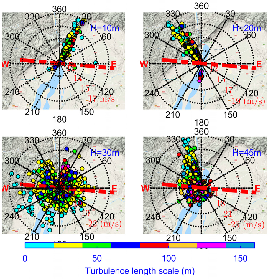
Turbulence integral scale.
It can be seen from Figure 9 that the larger turbulent integral scales are in the centre of the wind rose where the wind speed is lower. The turbulent integral scale changes significantly with the wind direction. For the wind direction in upstream or downstream of the river, the turbulent integral scale is slightly larger than the other directions. The turbulent integral scales are mostly within 160 m in the observed height.
Turbulence spectrum
The turbulence spectrum indicates the wind energy distribution over frequency


where

(a) Longitudinal fluctuating wind power spectrum at 30 m; (b) Longitudinal fluctuating wind power spectrum at 60 m; (c) Lateral fluctuating wind power spectrum at 30 m; (d) Lateral fluctuating wind power spectrum at 60 m; (e) Vertical fluctuating wind power spectrum at 30 m; (f) Vertical fluctuating wind power spectrum at 60 m; and (g) The fluctuating wind cross-spectrum at 60 m.
In Figure 10, the measured turbulence spectrum is compared with the Kaimal spectrum and the Simiu spectrum (Kaimal et al., 1972; Simiu and Scanlan, 1996). Figure 10(a) and (b) show that the along-wind average parameter spectrum at the 30 m height is larger than the Simiu spectrum and the Kaimal spectrum, while the average parameter spectrum agrees well with the Simiu spectrum at 60 m height. The energy of the average parameter spectrum at the two heights is higher than that of the Kaimal spectrum, which is shown in Figure 10(c) and (d). The energy of the vertical average parameter spectrum at the 30 m height is higher than that of the Simiu spectrum and the Kaimal spectrum. However, the vertical average parameters spectrum at the 60 m height is consistent with the Simiu spectrum in the low-frequency range. Figure 10(g) indicates that the energy of the fitted cross-spectrum is larger than that of the Kaimal spectrum.
Previous studies indicate that the velocity spectrum in the inertial subrange can be divided into a high frequency range, an intermediate frequency range and a low-frequency range (Drobinski et al., 2007). The difference is the value of
The m value wind rose.
Correlation analysis
To study the correlation of the fluctuating wind speed, the normalized cross-spectrum is introduced. It can be expressed as
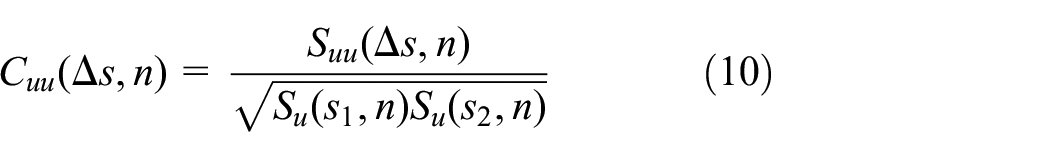
where

where
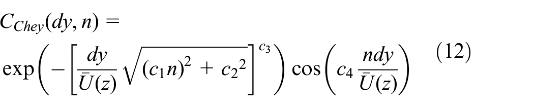
Obviously, if

(a) Normalized cross-spectra at 30 m; (b) Normalized cross-spectra between 30 m (Yellow River) and 45 m; and (c) Normalized cross-spectra between 30 m (Hejin) and 45 m.
Figure 12(a) shows that only the horizontal distance is considered, and the decay coefficient value suggested by Simiu is greater than the measured value. The suggested values of Simiu will overestimate the turbulence correlation overestimated in Figure 12(b). However, the fitted value in Figure 12(c) is close to the value suggested by Simiu.
Buffeting response
Coupled buffeting analysis
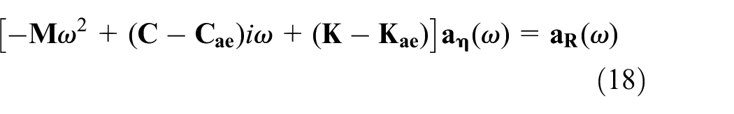
The bridge deck belongs to the horizontal line-like structure. The dynamic equation considering the influence of self-excited force is defined as (Cheynet et al., 2016)

where
Figure 4 shows that the strong wind direction mainly appears near 340°. Therefore, the recorded strong wind at the bridge site is skewed to the bridge axis, and the wind yaw angle

where
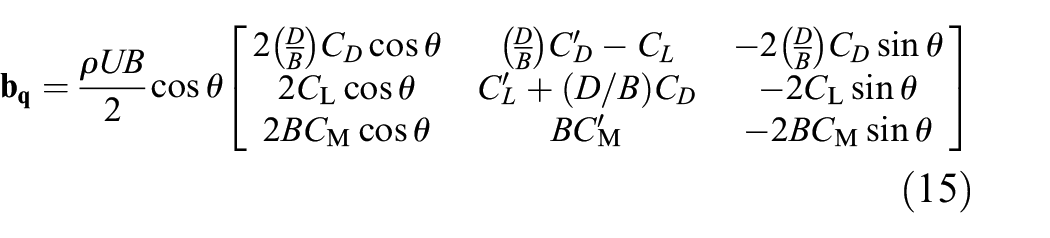
where
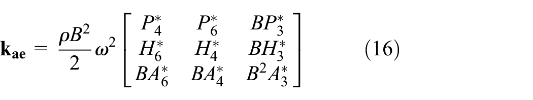

where

Test in the wind tunnel.
Taking the Fourier transform on either side of equation (13)
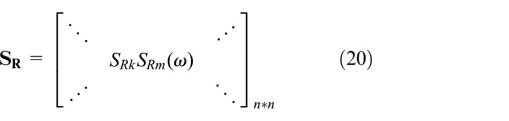
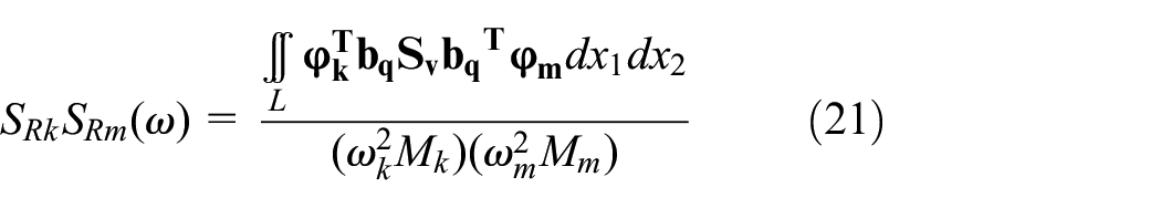
Therefore, the power spectral density of the bridge response at

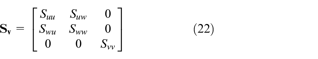
where
where
where

where
Modal analysis
The modal analysis of the bridge is performed using ANSYS software. The girder and towers are modelled by the Beam4 element, and the cables are treated as 3D tension-only truss elements (Link10). The secondary dead load is simulated by the Mass21 element. The nonlinear gravity stiffness of the cable is corrected by the Ernst equation (Ernst, 1965). The first 50 natural frequencies and mode shapes are calculated. The finite-element model and the typical modal shape are shown in Figures 14 and 15, respectively.

Finite-element model of the bridge.

Mode shapes of the bridge.
Buffeting results
According to the 29 consecutive years of wind data from the Hejin Meteorological Bureau, the basic wind speed is estimated to be 24.1 m/s by the generalized extreme value I type probability distribution. However, the Chinese Wind-Resistant Design Specification for Highway Bridges (JTG/T D60-01-2004) suggests a wind speed of 27.6 m/s. The power law index takes 0.1640. The first 20 modes are selected for the calculation. The vertical distance from the water surface to the middle cross section of the girder is 48.85 m. The buffeting response of the girder was calculated by using the Simiu spectrum, Kaimal spectrum and the fitted spectrum of 60 m height. Because the Simiu spectrum has no formula in the lateral direction, the lateral Kaimal spectrum are used. The fitted normalized cross-spectra in the range of 300°–360° of the Figure 12(b) is selected. The mean wind speed from field data is different from the wind resistant specification’s mean speed. First, we choose 27.6 m/s as the basic wind speed. For the sake of brevity, the aerodynamic admittance takes one. Figure 16 shows the root mean square (RMS) response of the bridge deck.
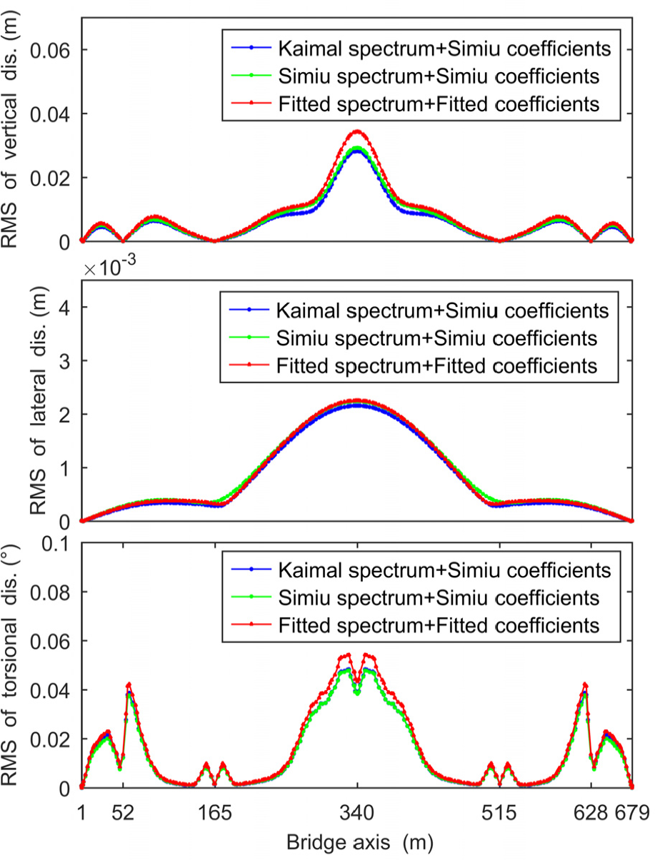
Influence of turbulence characteristics on RMS displacement.
Then, the different mean wind speeds are considered in the calculation of the buffeting response. Figure 17 shows the buffeting response at different mean wind speeds.

Influence of the mean speed on RMS displacement.
Finally, the mean wind speed is 24.1 m/s, and the turbulence spectrum uses the fitted spectrum. The effect of different types of aerodynamic admittance functions on the buffeting response is shown in Figure 18.
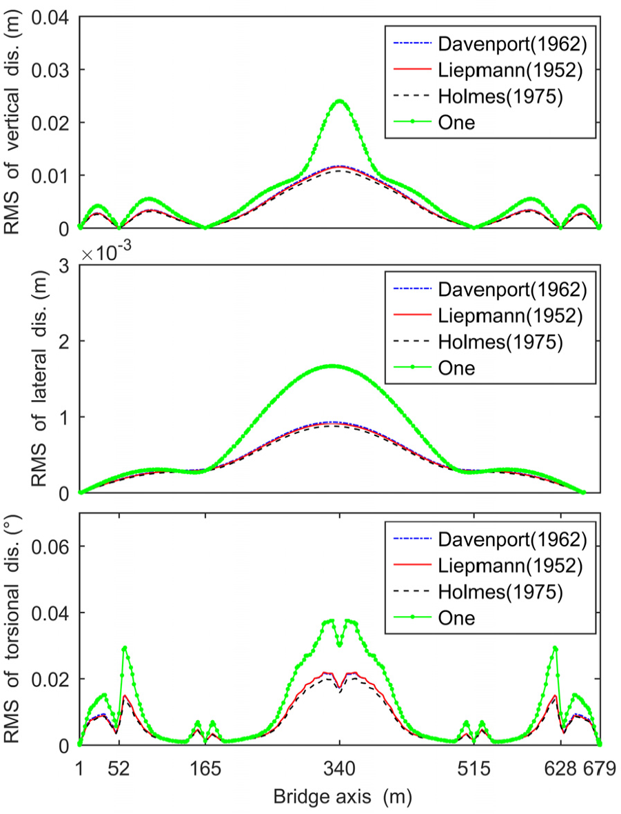
Influence of aerodynamic admittances on RMS displacement.
In Figure 16, the results indicate that with the Simiu spectrum and Kaimal spectrum, the buffeting response is underestimated, although the decay coefficient value suggested by Simiu is smaller than the fitted decay coefficient value. Compared with the turbulence spectrum value, the decay coefficients have few effects on the buffeting response in this study. Figure 17 shows that buffeting response is very sensitive to mean wind speed. When the mean wind speed changes by 3.5 m/s, its influence on the buffeting response will significantly exceed the influence of the different fluctuating wind characteristics on the buffeting response. Figure 18 shows that considering the aerodynamic admittance will significantly reduce the value of buffeting response. The aerodynamic admittance function proposed by Holmes has the largest reduction in buffeting response.
Conclusion
Strong wind characteristics and the buffeting response of the Longmen bridge located in a trumpet-shaped mountain pass were studied in this article by using the long-term monitoring wind data. The following main conclusions were reached:
The wind direction changes obviously with height, which means that the wind profile is extremely twisted. The turbulence intensity and turbulence integral scale are related to the wind direction. The relationship between turbulent intensity components in every two directions was investigated, and compared with existing conclusions.
The measured turbulence spectrum in both the longitudinal and vertical directions agreed well with the Simiu spectrum in the low-frequency range at the 60 m height. The magnitudes of the Kaimal spectrum in three orthogonal directions at both heights are lower than the measured spectrum. As noted in the article, there is no significant relationship between the
Only considering the horizontal distance, the Davenport’s model and Cheynet’s model satisfactorily represent the normalized cross-spectra of turbulence. For the different anemometers, a significant variation in the fitting value between 30 and 45 m can be found.
Using the Simiu spectrum or Kaimal spectrum will underestimate the buffeting response of the main girder when considering only the fluctuating wind characteristics. However, considering the difference between the measured mean wind speed and wind resistant specification’s mean speed, the result is the opposite. The aerodynamic admittance function can significantly reduce the buffeting response, but the difference of different types of aerodynamic admittance functions on the reduction of the buffeting response is small.
Footnotes
Declaration of Conflicting Interests
The author(s) declared no potential conflicts of interest with respect to the research, authorship, and/or publication of this article.
Funding
The author(s) disclosed receipt of the following financial support for the research, authorship, and/or publication of this article: This project was supported by the National Natural Science Foundation of China (Grant Nos. 51078038 and 51808052), Fundamental Research Funds for the Central Universities (300102219531), Natural Science Research Key Project of Anhui Provincial Higher Education (KJ2017A405).