Concrete crack detection and 3D mapping by integrated convolutional neural networks architecture

Abstract

This paper presents an image-based crack detection system, in which its architecture is modified to use deep convolutional neural networks in a feature extraction step and other classifiers in the classification step. In the classification step, classifiers including Support Vector machines (SVMs), Random Forest (RF) and Evolutionary Artificial Neural Network (EANN) are used as an alternative to a Softmax classifier and the performance of these classifiers are studied. The data set was created from various types of concrete structures using a standard digital camera and an unmanned aerial vehicle (UAV). The collected images are used in the crack detection system and in creating a 3D model of a sample concrete building using an image- based 3D photogrammetry technique. Then, the 3D model is used to create a mosaic image, in which the crack detection system was applied to create a global view of a crack density map. The map is then projected onto the 3D model to allow cracks to be located in the 3D world. A comparative study was conducted on the proposed crack detection system and the results prove that the combined architecture of CNN as a feature extractor and SVM as a classifier shows the best performance with the accuracy of 92.80. The results also show that the modified architecture by integrating CNN and other types of classifiers can improve a system performance, which is better than using the Softmax classifier.

Keywords

3D mosaic and crack mapping convolutional neural network crack detection image-based 3D modeling random forest support vector machine

Introduction

Cracks in concrete structures are initial signs of structure degradation and deterioration, and many structures are aging and required regular maintenance. Visual inspection is the most common procedure in a condition assessment for non-destructive evaluation (Chaiyasarn, 2014), although this method is laborious and time-consuming. The method normally involved experienced and skilled inspectors to assess the conditions of structures based on structures’ visual appearance. Therefore, there is an urgent need for an automatic system to facilitate and improve the visual inspection procedure. A number of image-based crack detection systems have been proposed aiming to detect cracks automatically and accurately as cracks can be difficult to identify in images due to their irregularity. Furthermore, various types of noises in images such as blemishes and shading, can add to the complexity of the crack detection tasks.

Previous crack detection systems generally extracted distinctive crack features, in which classifiers were applied to identify whether the features were cracks. Common features deployed for crack detection were blob detectors (Jahanshahi et al., 2013), edge detector (Abdel-Qader et al., 2003), Principal Component Analysis (Abdel-Qader et al., 2006), Gabor Filter (Zalama et al., 2014), scale space and intensity features (Prasanna et al., 2016), Local Binary Patterns (LBP) (Chen et al., 2017) and Wavelets (Bu et al., 2015). Although, crack detection systems based on features report some potential benefits (Lins and Givigi, 2016; Loupos et al., 2014), the performance of these systems relied on the art of choosing the right features, which only work with specific datasets.

Many recent crack detection systems are based on deep learning, which can extract features automatically from images, and the features are then classified in the last layer of the architecture by the Softmax classifier. Cha et al. (2017) proposed a system using a deep architecture of Convolutional Neural Network for detecting concrete cracks without manual crack features. Zhang et al. (2019) proposed context-aware deep convolutional semantic segmentation network to detect concrete cracks. Zhang et al. (2016) applied a Deep Convolutional Neural Network (DCNN) for detecting road cracks from images collected using a low-cost smartphone and demonstrated that the features obtained from DCNN were able to provide superior accuracy to handcrafted features. Zhang et al. (2017) proposed a CrackNet to detect pavement crack on the asphalt surface, and CrackNet outperformed 3D shadow modeling and pixel-SVM approaches. Ni et al. (2019) presented a crack detection system based on convolutional feature fusion and pixel-level classification, which showed promising results. Recent crack detection systems applied Fully Convolutional Neural Networks (FCN) to obtain pixel-level cracks (Alipour et al., 2019; Dung, 2019; Xue and Li, 2018), which showed accurate results with their datasets.

Integrated CNN architecture has demonstrated accuracy improvement in some previous works. In this framework, deep learning is used as feature extractors and alternative classifiers were used in the classification step. According to LeCun et al. (2015), multi-level deep features learned by CNN will likely replace traditional handcrafted features, and these features can then be classified with any classifiers. The alternative classifiers can be used instead of the Softmax to improve system performance as shown in Tang (2013), Alalshekmubarak and Smith (2013), and Agarap 2018). Ren et al. (2016) demonstrated that ensemble methods can provide more accurate predictions than using the Softmax layers. Chu and Chu (2019) integrated genetic programming with CNN features for the image classification task. Niu and Suen (2012) proposed a novel combined CNN-SVM approach for the handwritten recognition task by using features extracted from CNN and SVM as a classifier. Li et al. (2018) proposed a video-based crack detection system using the integration of CNN with a Naive Bayes data fusion system, and the system can detect defects more accurately and rapidly by a lightweight network method. Sharma et al. (2018) presented an improvement in crack detection when CNN was used as a feature extractor, which was then classified by Support Vector Machine. Therefore, in this paper, the integrated CNN architecture is proposed to automatically extract features, which are classified by alternative classifiers to improve crack detection accuracy.

Unmanned Aerial Vehicles (UAVs) have recently been used in the inspection as data collection tools, in which images are then processed offline by crack detection systems. Often, sites are not accessible, especially in tall structures, therefore UAVs are ideal tools in condition assessment applications since they can obtain data rapidly and offer more complete views of inspected sites (Torok et al., 2013). A number of previous inspection systems have incorporated the use of image-based techniques with UAVs to create a complete condition assessment system as demonstrated in Cha et al. (2017), Yoon et al. (2018), Sankarasrinivasan et al. (2015), Kang and Cha (2018). Morgenthal et. al. (2019) proposed a framework to use UAVs for conditional assessment in bridges. Liu et al. (2019) deployed a drone to obtain images, which were used to create 3D models for crack inspection of bridge piers, which can be used to localize the detected damages. Kalfarisi et al. (2020) presented a crack detection system, in which the cracks were integrated into a 3D reality mesh model to provide visualization of the detected cracks on sample concrete walls. Therefore, in this research, the detected cracks will be mapped onto a 3D realistic model so that inspectors can identify and verify the locations of the damages easily. This way, the proposed crack detection system with the integrated visualization of cracks on a 3D model can be a new tool for inspection reporting.

This paper proposes an automatic image-based crack detection algorithm, using an integration of CNN with alternative classifiers including Support Vector Machine (SVM), Random Forest (RF), and Evolutionary Artificial Neural Network (EANN) to increase classification accuracy. The system used a UAV and a handheld Digital Single-Lens Reflex (DSLR) camera as a data collection tool for images of concrete cracks. The results from crack detection are mapped onto a 3D model as a new way of inspection reporting. The contribution of this paper is twofold. Firstly, it is demonstrated that using alternative classifiers with the CNN architecture can improve CNN performance. The performance of CNN with different classifiers was also presented. And secondly, we present a new way of inspection reporting by mapping the detected cracks onto a realistic 3D model to provide better visualization for inspectors.

System overview

The outline of the proposed system is shown in Figure 1. The system consists of five modules, (1) Image acquisition via a drone and DSLR camera (Section 2.1), (2) Crack detection system (Section 3), (3) Image-based 3D modeling (Section 4.1), (4) Crack localization (Section 4.2) and (5) 3D Mapping (Section 4.3). The output of the system is a 3D model which shows regions containing cracks.

Figure 1.

The outline of the proposed crack detection system.

Image acquisition

UAVs have recently become tools in many tasks, for example, inspection and surveying methods, since they are cheaper, faster and more effective. In this proposed work, a DSLR camera and a drone Da-Jiang Innovations (DJI) Phantom 4 was used for data acquisition. To obtain images of a building for 3D modeling, the full coverage of a building was obtained by flying a drone in a pre-planned flight path called the Point of interest (POI) strategy as shown in Figure 1. In the POI strategy, a drone was programmed to fly around an object of interest at a predetermined radius and images were taken at approximately 2 to 3 s to ensure 50% overlap between consecutive images. The flight path was pre-programmed by Auto Flight Logic, which required radius, velocity, altitude, and camera viewing angles as input parameters. The flight was planned to ensure that it could perform tasks in specified battery time. To obtain close-up images of cracks, a drone was controlled manually to collect images of a building surface. Also, more images of cracks were also collected around many concrete buildings using a DSLR camera. The images of cracks will be used in the crack detection system as explained in Section 3.

Crack detection system

The outline of the proposed crack detection system is shown in Figure 1. The system consists of two modules, feature extraction and classification. In the proposed system, feature extraction is done by using Convolutional Neural Network (CNN), while Softmax, Support Vector Machine (SVM), Random Forest (RF) and Evolutionary Artificial Neural Networks (EANN) are used as classifiers. CNN have shown to outperform the method based on handcrafted features. The system takes image patches as input, in which features are extracted by CNN, and then, each classifier is employed to determine if the patches are crack or non-crack.

CNN-based feature extraction

Convolutional Neural Network (CNN) is a type of multi-layer feedforward Artificial Neural Network (ANN), which has two main parts, a multi-level deep feature extractor, and a classifier. The feature extractor consists of many layers, and the input to the feature extractor comes in the form of three 2D arrays, which are the image pixel intensity values RGB. The layers in the feature extractor obtain variance at each level in the form of discriminative features. The extracted features are then used to train the classifier. Generally, CNN used the Softmax classifier, but in the proposed work the architecture is modified by using SVM, RF, and EANN. The advantage of using CNN as a feature extractor is that it does not require any intervention in the design of multiple stage layers. These multiple layers are learned by using a learning procedure from raw data. Interested readers are referred to Goodfellow et al. (2016) and LeCun et al. (2015) for more detail.

CNN architecture

In the proposed work, Keras sequential model (Charles, 2013) is used for the CNN architecture, which consists of three-stage layers. The first few stages of CNN consists of three types of layers, convolutional layers, activation layer (ReLU) and max-pooling layers. The CNN architecture is designed in order to process the 2D grid-like topology of input images (Goodfellow et al., 2016) as shown in Figure 2(a). The first layer is the input with a pixel resolution of H×W×N, where H and W represent image height and width, and N represents the number of channels. The spatial size of the input data is reduced after passing from multiple convolutional and max-pooling layers in the architecture. Finally, the feature vectors are obtained from the fully connected layer, which is then given to the classifiers for prediction.

Figure 2.

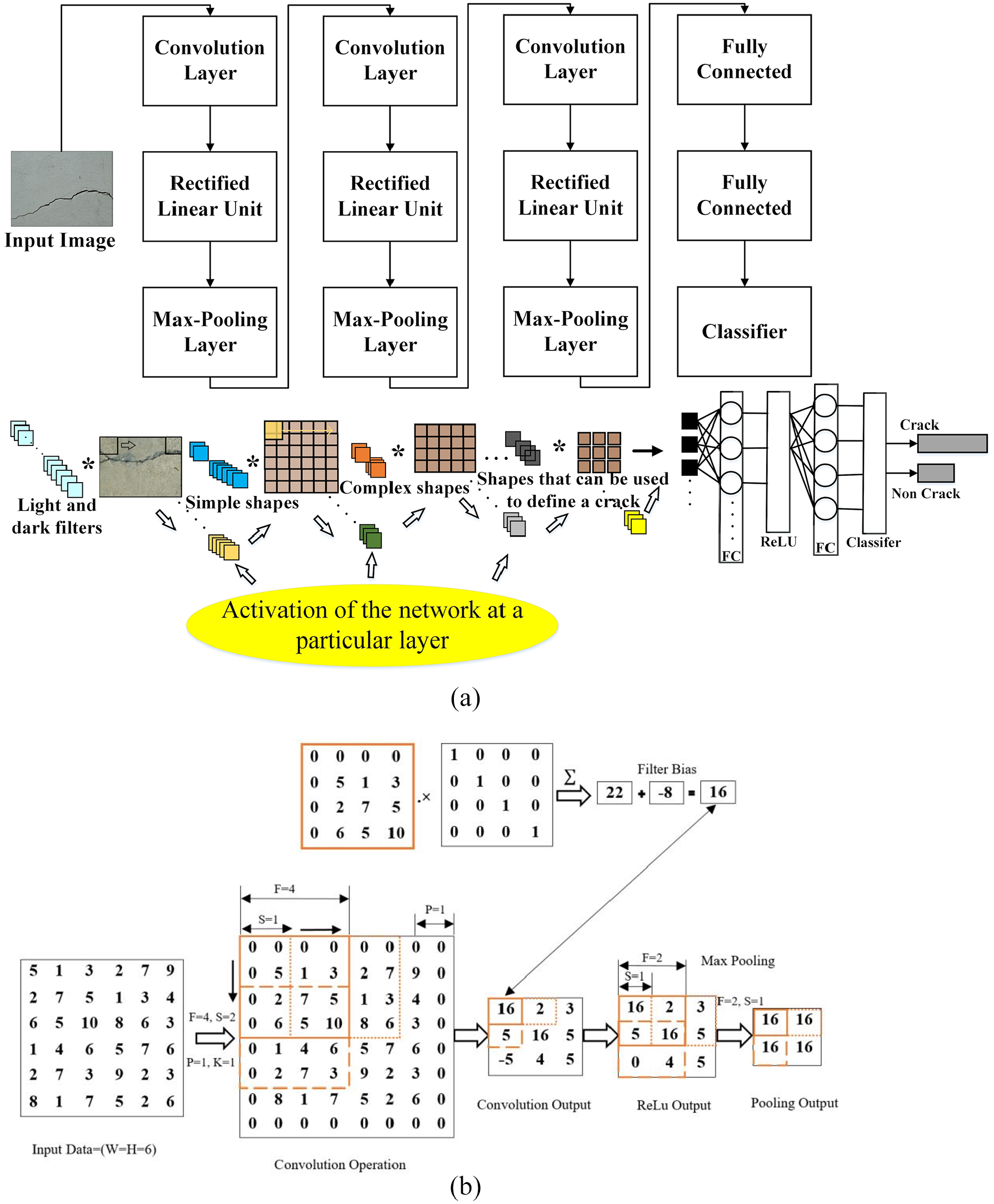
(a) The schematic diagram of the proposed CNN architecture, and (b) the illustration of the mathematical operation of the convolutional, ReLU and max pooling layers.

Convolutional layer

The convolutional layer takes an image as input data and performs three operations on the input data as shown in Figure 2(b). The primary role of the convolution layer is to find a local connection of features from the previous layer as described in equation (1).

O = \sum (I_{F \times F} . w_{F \times F}) + b

(1)

The convolutional operation is performed on the local receptive field I_{F ×F} and the output O is obtained. The filter weights are represented by w_{F ×F}, in which F is a kernel window size of the local field. The filter bias is represented by b. The obtained feature maps are then passed to the activation layer (ReLU).

Activation layer (ReLU)

After the convolution layer, the activation layer ReLU (Rectified Linear Units) (Figure 2(b)), introduced by Nair and Hinton (2010), is applied. This layer couples non-linearity to the system since the ReLU output is not bounded to the output values, except for the negative input values, and its gradients are either zeros or ones. From these properties, the ReLU function offers a faster computation capability than other ordinary non-linear functions such as the Sigmoid function. The operation of this ReLU activation layer is depicted in equation (2).

σ (i) = m a x (0, i)

(2)

where i is the elements of the input vectors.

Max-Pooling layer

As shown in Figure 2(b), the max-pooling layer performs a downsampling operation by dividing an input image into small non-overlapping rectangular blocks. Then, the maximum value of each block is computed. The max- pooling operation is used for two purposes, (1) reducing non-maximal values which helps to decrease computational time, and (2) a down-sampling the size of a feature vector.

Fully connected layer

The function of the fully connected layer is to compute the class scores. In this work, the output of the fully connected layer is the input feature vector for other classifiers. The output of the fully connected layer is shown in equation (3)

Y_{b \times 1} = W_{b \times a} . I_{a \times 1} . B_{b \times 1}

(3)

where W and B represent the weight and bias matrix. b and a are the sizes of the output and input vector, and the output of the fully connected layer is represented by Y.

CNN training

CNN training increases feature variation which helps to avoid the over- fitting problem. The dropout method is used for CNN training to reduce the possibility of over-fitting as suggested in Srivastava et al. (2014). The input to CNN is an image patch of size r × r × d, where r is the height and width of the image patch and d = 3 is number of channels in RGB. The training dataset is {I_n, y_n}, n = 1, 2, …, m and m is the total number of image patches, I_n is an image patch and y_n is a class label {1, 0}. The first convolutional layers consist of 32 convolutional filters of size 3 × 3, and the max pooling filters have a ratio of 2. CNN training is stopped after 20 epochs when the loss is converged to a fixed value as shown in Figure 9.

Classifiers

Softmax

Softmax is the last layer of CNN architecture and is typically used for classifying input data. The Softmax classifier provides normalized class probabilities as shown in equation (4)

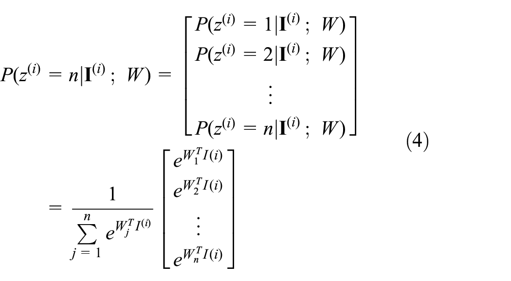
\begin{matrix} P (z^{(i)} = n | I^{(i)}; W) = [\begin{matrix} P (z^{(i)} = 1 | I^{(i)}; W) \\ P (z^{(i)} = 2 | I^{(i)}; W) \\ ⋮ \\ P (z^{(i)} = n | I^{(i)}; W) \end{matrix}] \\ = \frac{1}{\sum_{j = 1}^{n} e^{W_{j}^{T} I^{(i)}}} [\begin{matrix} e^{W_{1}^{T} I (i)} \\ e^{W_{2}^{T} I (i)} \\ ⋮ \\ e^{W_{n}^{T} I (i)} \end{matrix}] \end{matrix}

(4)

For i = 1,2…m, where m, n, and W represent the number of training samples, the number of class and weights, respectively, ${W_{n}}^{T} I^{(i)}$ represents inputs to the classifier, which in this work, it is a feature vector from the fully connected layer. Equation (4) takes a vector of arbitrary real-valued scores and squashes it to a vector to values between 0 and 1.

Support vector machine

Support Vector Machine (SVM) is a supervised learning method whose objective is to obtain the optimal decision boundary to separate data in the multi-dimensional space or binary classification (see Cortes and Vapnik, 1995). The optimal decision boundary is a boundary which is the furthest distance from the vectors nearest to the boundary between the two sets of data as exemplified in Figures 3 to 5. The training set of samples for the SVM classifier is given by equation (5)

S = {({\bar{x}}_{i}, y_{i}) | ({\bar{x}}_{i}, y_{i}), i = 1, 2, . . ., m}

(5)

where x_i is the input feature for the ith sample and y: ∈ {1, 0} is the class label for the i^th sample. Hence, the dataset S is linearly separated by a hyperplane as shown in equation (6).

{\bar{w}}^{T} . \bar{x} + b = 0

(6)

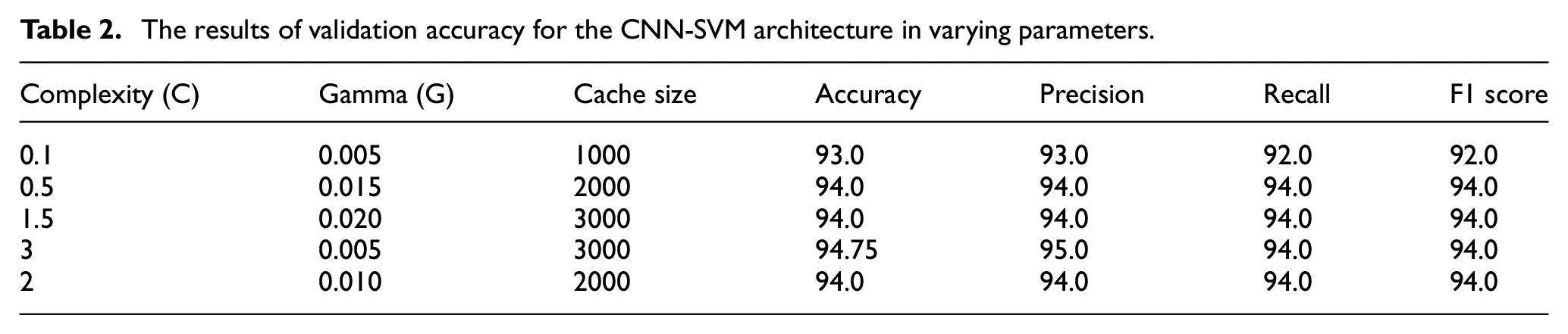
where w is the weight or the direction of the linear decision boundary, and b is an added bias, which is required to maximize the margin between each class. In the proposed system, SVM takes output features from CNN’s fully connected layer as input features, and a Radial Basis Function (RBF) kernel is used to map the features from non-linear to a linear space. To obtain the optimal values for the kernel, a cross-validation technique has been employed. In the proposed work, a different combination of C and gamma values were tried using the validation data set to obtain maximum accuracy.

Figure 3.

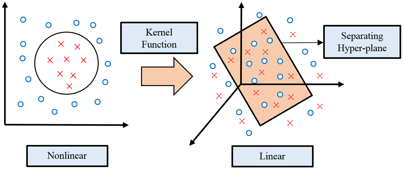
An illustration of support vector machine.

Figure 4.

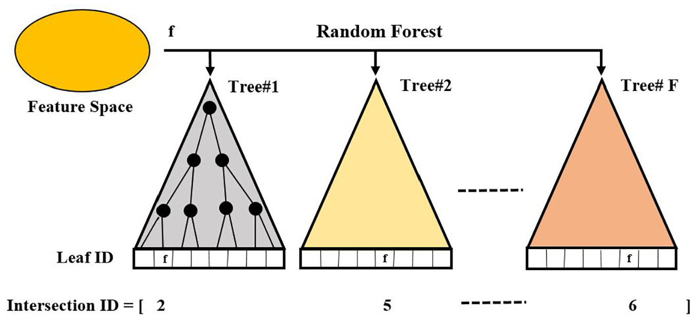
The schematic diagram of random forest.

Figure 5.

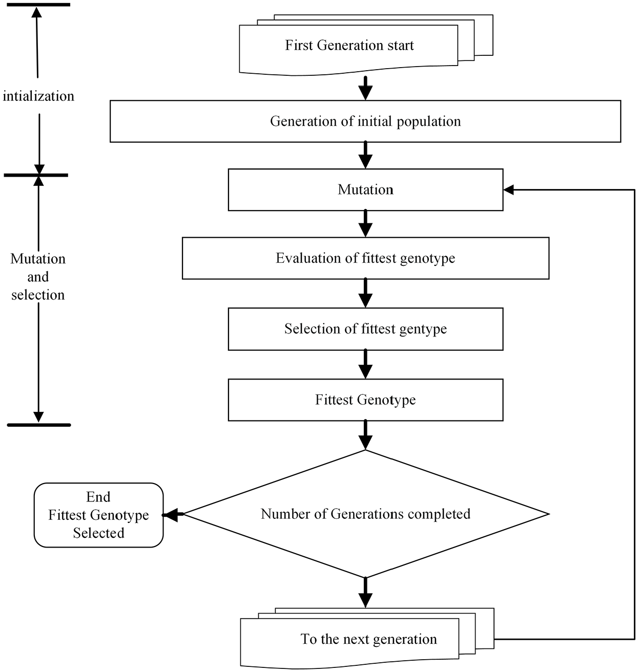
The process diagram of the genetic algorithm.

Random Forest

Random Forest is a supervised learning method based on a combination of bagging and random feature space algorithms. It classifies features into different class clusters so that the same features within the same class clusters are said to have similar characteristic features in order to qualify to be in the same clusters. As shown in Figure 6, a forest T can be looked as a composition of decision trees f_t. Each decision tree f_t(x) gives the prediction of a sample x∈X, which classifies a sample x by recursively branching left or right down the tree until the last leaf node of the decision tree denoted by L(π) ∈ f_t is reached. π is the most represented description sets of predicted class label distributed over Y, where y∈Y that is, each split node $N (h, {f_{l}}^{T}, {f_{l}}^{R}) \in f_{t}$ is associated with the decision stump (binary split function).

h (x, θ_{l}) \in f_{t}

(7)

In equation (7), θ_l are features for each node l. If h(x, θ_l) = 0, sample x should be branched to left sub-tree $f_{l}^{T}$ , otherwise it goes to the right sub-tree $f_{l}^{R}$ . In the proposed system, the fully connected layer output is an input as a new feature vector for RF. The validation dataset is used to optimize parameters, particularly the number of estimators E, the maximum depth of tree D, and the minimum sample split M. To choose suitable parameters of the RF classifier, that is, M, E, and D, a different combination of values was tried using the training and validation data.

Figure 6.

The example images of crack and non-crack patches for various types of concrete surface in the dataset used in this proposed work.

Evolutionary Artificial Neural Network

Evolutionary Artificial Neural Network (EANN) is the ANN that is trained by a Genetic Algorithm (GA) and evolutionary programming. In EANN, GA algorithm is called Genotype, ANN is called Phenotype, and connecting weights are named as genes. The genotype finds the connecting weights for the phenotype. The overall process consists of initialization, mutation, and selection as shown in Figure 7. In initialization, the genotype is made from all weights of the EANN architecture, and random values are assigned by a random generator ranging from −1 to 1. From the parent genotype, offspring are created in the process of mutation. The number of produced offspring depends on the population size. Amongst the mutated genotypes, the best one is selected in the selection process, and the associated weights are fixed into the ANN phenotype.

Figure 7.

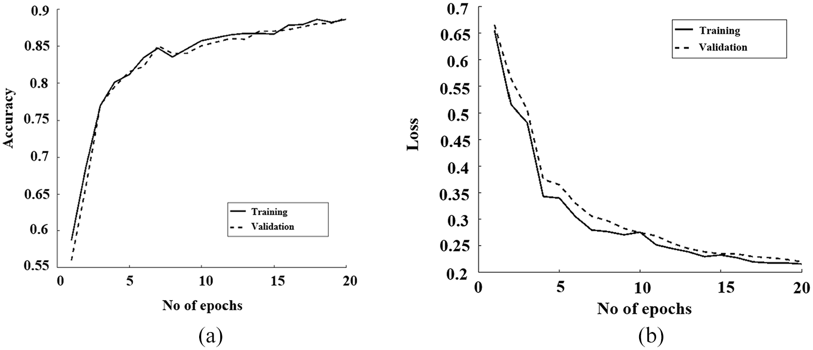
(a) The plot of CNN accuracy and (b) the plot of CNN loss.

In the EANN classifier, each row represents the features of a single image known as a chromosome, which is normalized to make the string binary. When initialization takes place, the parent genotype is created, and random values are assigned to this genotype between 0 and 1. After the initialization process, mutation takes place. In this research work, the mutation rate is set as 10%, and the population size is set as 5. Four offspring are produced from a single parent genotype. In selection fitness, each string or chromosome is tested individually and is rated. After all genotypes are tested, the best one is selected by comparing the counts, and the fittest one is selected. The process of mutation and selection will take place after 1 million times, in which the fittest genotype is selected. After training the EANN classifier, it is tested to determine to see if it can identify whether a given image is cracked or non-cracked. The output of the testing data is calculated and compared with target values to evaluate the performance of the EANN algorithm.

Mosaicing and 3D crack mapping

Image-based 3D modeling

The outline of an image-based 3D modeling system is shown in Figure 1. The system consists of three stages, Feature Extraction and Matching, Structure from Motion (SfM) and Dense Reconstruction. Feature Extraction refers to the extraction of relevant information from images. Various distinctive features in images include corners, blobs, edges, or local image patches with particular properties. One of the prominent features extraction algorithm, which is used in this research work, is Scale Invariant Feature Transform (SIFT) (Lowe, 2004). Once the features are detected, a feature descriptor algorithm is applied to create the descriptor vectors to represent the appearances of the features. The descriptors are matched by feature matching algorithms to establish correspondences, which are filtered by robust matching algorithms. In this research work, the matching algorithm is performed by a brute-force search algorithm and the robust algorithm is RANdom Sample Consensus (RANSAC) for the fundamental matrix, and the interested reader can be referred to Lowe (2004) for details.

The matching step is done on pairs of images across all images in the database to generate tracks. These tracks are used to initialize the optimizer by a triangulation technique, which estimates the sparse point cloud and camera poses by the overlaps of image triplets. Then, the sparse point cloud and the camera poses are refined by Bundle Adjustment (BA). The BA algorithm iteratively adjusts the positions of the 3D coordinates and the camera poses to minimize the sum of the distances between the re- projections of the reconstructed 3D points through the estimated cameras, and the real image features coordinates (Soga, 2007). The output from SfM is used as the initializer to an algorithm Patch-based Multi-view Stereo (PMVS), which takes a set of images and camera parameters from SfM, and then reconstructs a sparse model to a dense 3D point cloud. PMVS algorithm is the backbone of most dense cloud algorithm. Interested readers are referred to Furukawa and Ponce (2009) for a detailed explanation. Agisoft was applied in this stage in this research work.

Mosaicing

Mosaic image increases the field of view of a scene, which cannot be achieved with a single image. For inspection, a single image does not give inspectors a spatial sense; hence, it is difficult to indicate the locations of any observed anomalies from an individual image. In this proposed work, a mosaic image of a building is created using the camera calibration from the image-based 3D modeling step (See Section 4.1 and Figure 1). Mosaicing starts by image warping, in which images are rectified by transformation matrices. Since all camera calibrations are known from the previous step, images are warped onto a selected mosaicing plane by a re-projection method. Then for the final stitched image, different processes are applied including selecting a compositing surface, selecting pixel contributions to the final composite, and blending these pixels to minimize any visible seams, blur and ghosting. Agisoft is employed in this process.

Crack localization

Crack regions are localized by a simple sliding window technique. As shown in Figure 1, a chosen window size m×n is selected, which is slid over a target image to perform a search. Each patch is classified by the trained crack detector (explained in Section 3). The window moves by m/2 pixels after classifying an image patch. If the patch is classified as crack, the patch is highlighted in an image. In the proposed work, crack localization is performed on a mosaic image, which is then mapped onto the 3D Model to visualize cracks in 3D world coordinates.

3D crack mapping

3D mapping is the process to map a 2D image onto a 3D model. The mapping can enhance visualization and allows cracks regions to be localized in the 3D world. Once the crack regions are localized in the mosaic image, it is mapped onto a 3D model (see Figure 1) by the re-projection method using equation (8). Only a planar surface in the 3D model can be mapped as other types of surface requires different techniques of texture mapping.

X_{i} = {P_{i}}^{- 1} x_{i}

(8)

From the equation above, P is a projection matrix of an ith camera, x is the image coordinate, and X is a 3D coordinate.

Experiments and results

Crack detection

Image database

To extract features by CNN, image patches are assigned label manually as crack or non-crack. Images are converted into patches of size 32 × 32. As exemplified in Figure 8, the sample patches of cracks contain predominantly visible cracks within the patches and the non-crack patches are only simply image patches of concrete surface. Various types of concrete surface are collected as samples for the proposed system. A total of 16,000 patches are created with 50% crack patches and 50% non-crack patches. The patches were split into training, validation and testing data with the split ratio of 6:2:2, respectively and the split for validation is chosen randomly when we calculated the accuracy of the system. For training and validation, five-fold cross validation was applied.

Figure 8.

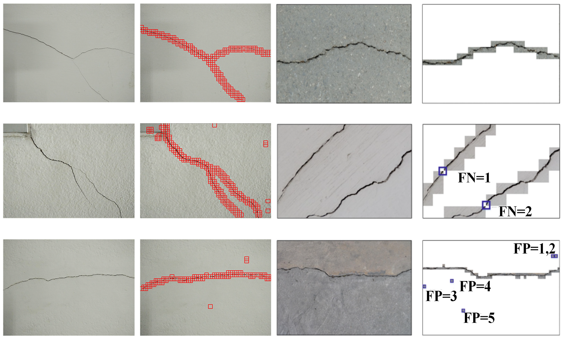
The second column shows an example of the localization of crack regions by the CNN-SVM architecture using the sliding window technique, and the fourth column shows the example of testing results when scanning for the locations of False Positive (FP) and False Negative (FN).

Classification results

Figure 9(a) and (b) shows the accuracy and loss graphs of CNN to evaluate the performance of the CNN-Softmax model. As shown in the plots, for both training and validation, accuracy and loss become stable after running the model for 20 epochs.

Figure 9.

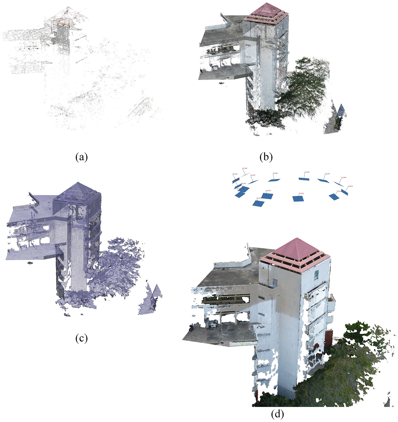
The figure shows steps in creating the 3D model: (a) sparse point cloud, (b) dense point cloud, (c) a mesh model, and (d) a texture 3D model and camera calibrations of a concrete building created from drone images using the POI strategy, not all cameras are shown for clarity.

The experiments were conducted by comparing the results obtained from different integrated CNN architecture, namely, CNN-Softmax, CNN-SVM, CNN-RF, and CNN- EANN. Table 1 shows the results of CNN features with RF classifiers. A parametric study was performed for RF classifier and the best validation and testing accuracy of 90.17% and 89.10% (see Table 4). The optimal parameters for RF were obtained on keeping the value of E = 50, D = 15, and S = 2 respectively. For the CNN-SVM architecture, the Radial Basis Function (RBF) was used as a kernel, and a cross-validation technique was employed to obtain the optimal values for the kernel. Table 2 shows a parametric study of SVM. And it can be seen that optimal validation is 94.75% when occurred at C = 3 and G = 0.005. And from Table 4, the testing accuracy is 92.80%. For the CNN-EANN architecture, the network size was varied, and the optimal validation and testing accuracy is 91.75% and 90.10%, respectively, when the network size of 3 × 3 and seed value 0 was kept as shown in Tables 3 and 4.

Table 1.

The results of validation accuracy for the CNN-RF architecture in varying .parameters.

Estimator (E)	Max depth (D)	Min split (S)	Validation accuracy
30	10	2	89.5
50	10	2	89.6
50	15	2	90.1
70	10	2	89.4
80	10	2	89.3

Table 2.

The results of validation accuracy for the CNN-SVM architecture in varying parameters.

Complexity (C)	Gamma (G)	Cache size	Accuracy	Precision	Recall	F1 score
0.1	0.005	1000	93.0	93.0	92.0	92.0
0.5	0.015	2000	94.0	94.0	94.0	94.0
1.5	0.020	3000	94.0	94.0	94.0	94.0
3	0.005	3000	94.75	95.0	94.0	94.0
2	0.010	2000	94.0	94.0	94.0	94.0

Table 3.

The results of validation accuracy for the CNN-EANN architecture in varying parameters.

Seed value	Network size	Validation accuracy	Testing accuracy	Detection rate	False alarm
0	2 × 2	91.31	90.00	98.0	16
1	2 × 2	92.68	90.00	98.0	16
0	3 × 3	91.20	90.10	97.0	15
1	3 × 3	91.75	90.25	96.0	14

Table 4.

The results show the optimal validation and testing accuracy for all architectures with an average processing time over 5468 patches extracted from a 2800 × 2000 image.

Architecture	Validation accuracy	Testing accuracy	Average time (second)
CNN-Softmax	89.39	88.25	0.003
CNN-SVM	94.75	92.80	0.250
CNN-RF	90.17	89.10	0.290
CNN-EANN	91.75	90.25	5.000

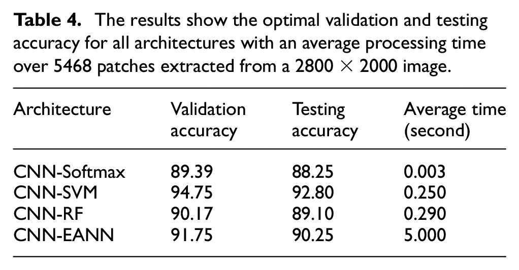
Then, the features obtained from the fully connected layer were given as input to other classifiers. From Table 4, the CNN-Softmax model, the accuracy is 89.39% for validation, and the testing result is 88.25%. The CNN-SVM architecture offers the best validation and testing accuracy of 94.75% and 92.80%, respectively, which is an improvement from the CNN-Softmax architecture. Other metrics, including Precision, Recall, and F1Score are also better for the CNN-SVM architecture. The CNN-SVM accuracy value is greater than the accuracy of the CNN-Softmax, CNN-RF, and CNN-EANN techniques by 4.55%, 3.70%, and 2.55% respectively. Table 4 also shows an average time for the classification of a single patch. Here, 5468 test patches extracted from a 2800x200 image were tested to calculate an average time for each architecture. It can be seen that the CNN-Softmax architecture took the least amount of time of 0.003 s, whereas the CNN-EANN architecture took the longest time.

Crack localization

The performance of CNN-SVM in localizing crack regions is examined by giving test images that are not used in the training and validation step. The images are collected from various types of concrete surface. Figure 10 shows the testing results of CNN-SVM architecture in localization crack regions by the sliding window technique. The areas inside the red boxes indicate that cracks are detected in the areas. It can be seen that, in all images, most crack regions are correctly identified. Furthermore, the integrated architecture of CNN-SVM shows excellent accuracy for various types of cracks.

Figure 10.

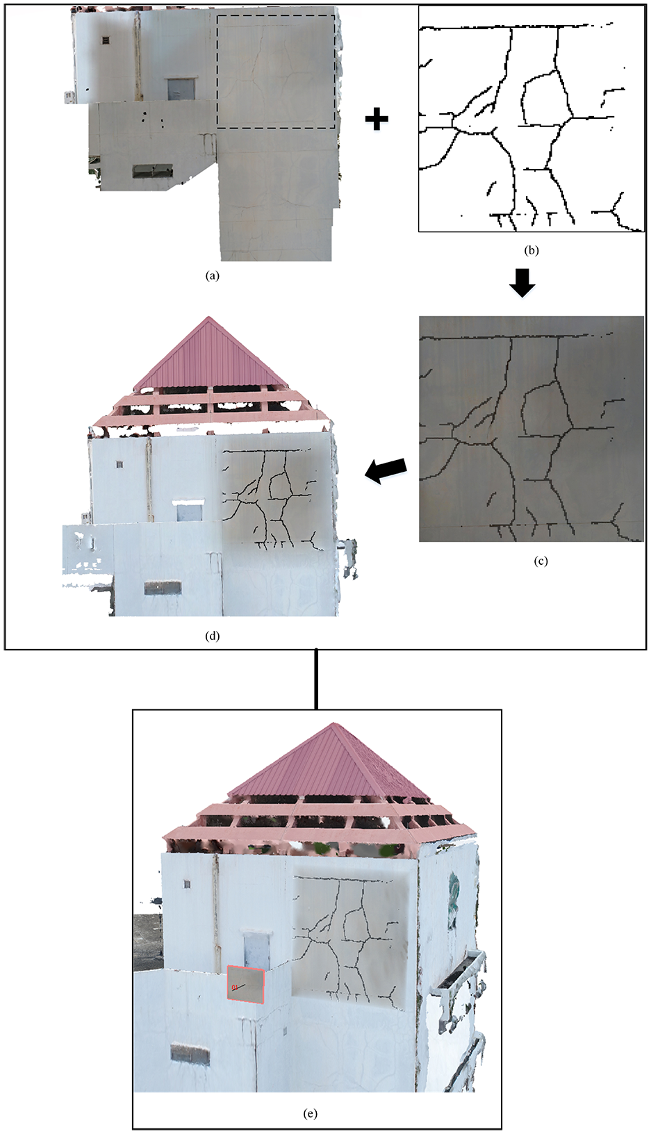
The steps in 3D Mapping: (a) an original mosaic image, (b) a binary map showing crack regions from the crack detection system, (c) a real texture image with the binary mask overlaid on the original mosaic image (d) a mosaic image with localized crack regions, and (e) a 3D model with the localization of crack regions.

Additionally, Figure 10 shows the results of crack localization when scanning results for the regions of False Positive (FP) and False Negative (FN) in testing images. The dark blue color boxes represent the FP and FN regions. As can be observed, there is fewer number of FN patches than the FP patches. The majority of FP patches are located in the regions where the surfaces mostly resemble cracks. These regions include shadows, air bubbles on the surface, discoloration, and water patches. These regions can be complex to distinguish for CNN.

3D crack mapping

The CNN-SVM architecture was applied in the test data on a concrete building to localize crack regions in 3D and then combine with a 3D model to exemplify a novel approach for inspection reporting.

Image-based 3D modeling and Mosaicing

Figure 9 shows the 3D model of a building and image locations obtained by a drone using the pre-programmed POI strategy to obtain the overview of the building. As can be seen from the figure, the texture of the building is realistic and is sufficient inspection. The 3D model was created by Agisoft PhotoScan, which requires four steps in the construction of the model as shown in Figure 9.

Firstly, a sparse point cloud is created from Structure from Motion, then the camera calibrations from the previous step is used to generate a denser point cloud. The dense point cloud is used to create a mesh, which is textured map in the final step to obtain a realistic 3D model as shown in Figure 9. The 3D model was created from 108 4864 × 3864 images, and the 3D model is created from 22,096 out of 23,630 tracks with the Root Mean Square (RMS) and maximum re-projection errors of 0.170 and 0.57 pixels, respectively. The number of 3D points of the dense point cloud is 32,263,168 and 1,194,870 points are used as vertices for the mesh.

Figure 10(a) shows the results of a mosaic created from the 3D model by Agisoft. A plane is chosen as an interested view of the building, and then a mosaic image is created by re-projecting the texture from images onto the plane. It can be seen that the quality of the obtained mosaic image realistic and almost distortion-free. In this work, the mosaic image is of size 27643 × 27332 pixels with 31.2 MB.

Crack localization and mapping

We applied our crack detection system on some region of the mosaic image as shown in Figure 10. Figure 10 shows the steps involved in the mapping onto the 3D model. Once, the mosaic is localized by the crack detection system (Figure 10(b) and (c)), then the 3D model is texture-mapped (Figure 10(d)). As shown in Figure 10(e), the 3D model has been highlighted with crack regions, which can be used as part of an inspection report. This enables inspectors to know the locations of cracks in the 3D sense, which is extremely useful for inspection.

Discussion

The combined models show an increase in accuracy as shown in Table 4. The proposed research shows that better classification performance can be achieved when combining CNN with a classifier. It can be seen that cracks can be detected automatically in a mosaic image and are useful for inspecting concrete structures. The system can identify cracks in a high resolution image mosaic to create the global view of a crack map, which has not been conducted in the previous crack detection systems. A closer inspection of Figure 10(e), the crack regions as detected by the proposed system contain the pattern of hairline cracks, which may be due to concrete curing. The proposed system allows inspectors to be able to examine these problematic regions more closely.

The proposed research shows the usefulness of an automated system in inspecting concrete structures and offers a novel approach for inspection reporting. The system keeps the database of concrete structures as well as providing the current state of the structures. The system allows structures to be inspected more thoroughly and images can be used to update the model to provide an up-to-date version of a structure. This system demonstrates the use of technology in the inspection of concrete structures and the advancement in automation.

The system proposed here can be a prototype for a fully automatic robotic system for inspection. CNN is capable of extracting discriminative features from a large number of images without any pre-processing. However, a large amount of training data is required, which can be considered as a disadvantage. Although CNN is extremely good at extracting features and classification, it relies on good data sets. Nevertheless, CNN has proved to be the best method for classification, especially for the crack detection task.

The 3D mapping technique proposed in this work is limited for the projection onto a planar surface. It is possible to map the image onto other types of geometrical surface, cylinder, sphere or cone, by a texture mapping technique using openGL, McReynolds and Blythe (2005).

The proposed method can currently localize cracks on a concrete surface. In order to obtain the sizes of cracks (i.e. length and width), pixels that belong to crack regions must be extracted. This can be achieved by other pixel-level techniques based on intensity, edge features, or deep learning techniques (Abdel-Qader et al. 2003; Zhang et al. 2017). However, these techniques are generally applied to smaller regions since they require more computational efforts. The proposed method in this work can be applied as a pre- processor to quickly identify crack locations, and then the pixel-level methods can be employed to improve the speed and accuracy of crack detection systems.

Conclusion

From the discussion, it can be concluded that the proposed crack detection system together with the drone technology can be applied in inspecting damages, especially cracks, from the images of concrete structures. The system employed the drone technology and a standard digital camera to acquire images, which are then processed by the crack detection system. The system is capable of localizing crack in a large mosaic image to create a global view of crack map and the 3D model with the localized mapping offers a novel way of inspection reporting, which provides a better view and a sense of space for inspectors. This can increase the effectiveness in the long term monitoring of concrete structures.

It can be concluded that, for the crack detection task, the integrated architectures of CNN-SVM, CNN-RF, and CNN-EANN are better than the CNN-Softmax model. From the results the CNN-SVM model gives the best accuracy in both validation and testing data sets. Therefore, it can be concluded that, for the classification problem, CNN should be employed in the feature extraction process and classifiers can be replaced by any techniques.

Footnotes

Acknowledgements

The author would like to thank Mr Luqman Ali for helping with experimental works.

Declaration of conflicting interests

The author(s) declared no potential conflicts of interest with respect to the research, authorship, and/or publication of this article.

Funding

The author(s) disclosed receipt of the following financial support for the research, authorship, and/or publication of this article: The work is supported by Thailand Research Fund, grant number MRG6080222. The last author would like to acknowledge the Ratchadapisek Sompoch Endowment Fund (2020), Chulalongkorn University (763014 Climate Change and Disaster Management Cluster).

ORCID iD

Suched Likitlersuang

References

Abdel-Qader

Abudayyeh

Kelly

(2003) Analysis of edge-detection techniques for crack identification in bridges. Journal of Computing in Civil Engineering 17(4): 255–263.

Abdel-Qader

Pashaie-Rad

Abudayyeh

, et al. (2006) PCA-based algorithm for unsupervised bridge crack detection. Advances in Engineering Software 37(12): 771–778.

Agarap

(2018) A neural network architecture combining gated recurrent unit (GRU) and support vector machine (SVM) for intrusion detection in network traffic data. In: Proceedings of the 2018 10th international conference on machine learning and computing, 26–28 February 2018. pp.26–30. NewYork: Association for Computing Machinery.

Alalshekmubarak

Smith

(2013) A novel approach combining recurrent neural network and support vector machines for time series classification. In: 2013 9th international conference on innovations in information technology, Abu Dhabi, 17–19 March 2013, pp.42–47. New Jersey: IEEE.

Alipour

Harris

Miller

(2019) Robust pixel level crack detection using deep fully convolution neural networks. Journal of Computing in Civil Engineering 33(6): 04019040.

Chanda

Guan

, et al. (2015) Crack detection using a texture analysis-based technique for visual bridge inspection. Electronic Journal of Structural Engineering 14(1): 41–48.

Cha

Choi

Büyüköztürk

(2017) Deep learning-based crack damage detection using convolutional neural networks. Computer-Aided Civil and Infrastructure Engineering 32(5): 361–378.

Chaiyasarn

(2014) Damage detection and monitoring for tunnel inspection based on computer vision. Doctoral Thesis, University of Cambridge, Cambridge. Available at: https://doi.org/10.17863/CAM.14071

Charles

(2013) GitHub repository. Available at: https://github.com/charlespwd/project-title

10.

Chen

Jahanshahi

, et al. (2017) A texture-based video processing methodology using Bayesian data fusion for autonomous crack detection on metallic surfaces. Computer-Aided Civil and Infrastructure Engineering 32(4): 271–287.

11.

Chu

(2019) A genetic programming approach to integrate multilayer CNN features for image classification. In: International conference on multimedia modeling, 8–11 January 2018, Cham: Springer, Thessaloniki, Greece, pp.640–651. Cham: Springer.

12.

Cortes

Vapnik

(1995) Support-vector networks. Machine Learning 20(3): 273–297. DOI: 10.1007/BF00994018.

13.

Dung

(2019) Autonomous concrete crack detection using deep fully convolutional neural network. Automation in Construction 99: 52–58.

14.

Furukawa

Ponce

(2009) Accurate camera calibration from multi-view stereo and bundle adjustment. International Journal of Computer Vision 84(3): 257–268.

15.

Goodfellow

Bengio

Courville

(2016) Deep Learning. Cambridge, MA: MIT Press.

16.

Jahanshahi

Masri

Padgett

, et al. (2013) An innovative methodology for detection and quantification of cracks through incorporation of depth perception. Machine Vision and Applications 24(2): 227–241.

17.

Kang

Cha

(2018) Autonomous UAVs for structural health monitoring using deep learning and an ultrasonic beacon system with geo-tagging. Computer-Aided Civil and Infrastructure Engineering 33(10): 885–902.

18.

Kalfarisi

Soh

(2020) Crack detection and segmentation using deep learning with 3D reality mesh model for quantitative assessment and integrated visualization. Journal of Computing in Civil Engineering 34(3): 04020010.

19.

LeCun

Bengio

Hinton

(2015) Deep learning. Nature 521(7553): 436–444.

20.

Huang

Xie

, et al. (2018) Research on a surface defect detection algorithm based on MobileNet-SSD. Applied Sciences 8(9): 1678.

21.

Lins

Givigi

(2016) Automatic crack detection and measurement based on image analysis. IEEE Transactions on Instrumentation and Measurement 65(3): 583–590.

22.

Liu

Nie

Fan

, et al. (2019) Image-based crack assessment of bridge piers using unmanned aerial vehicles and three-dimensional scene reconstruction. Computer-Aided Civil and Infrastructure Engineering 35(5): 511–529.

23.

Loupos

Amditis

Stentoumis

, et al. (2014) Robotic intelligent vision and control for tunnel inspection and evaluation-The ROBINSPECT EC project. In: International symposium on robotic and sensors environments (ROSE), Timisoara, Romania, 16–18 October. New Jersey: IEEE

24.

Lowe

(2004) Distinctive image features from scale-invariant keypoints. International Journal of Computer Vision 60(2): 91–110.

25.

Morgenthal

Hallermann

Kersten

, et al. (2019). Framework for automated UAS-based structural condition assessment of bridges. Automation in Construction 97: 77–95.

26.

Nair

Hinton

(2010) Rectified linear units improve restricted boltzmann machines. In: Proceedings of the 27th international conference on machine learning (ICML-10), 21–24 June 2010, Haifa, Israel, pp.807–814.

27.

Zhang

Chen

(2019) Pixel-level crack delineation in images with convolutional feature fusion. Structural Control and Health Monitoring 26(1): e2286.

28.

Niu

Suen

(2012) A novel hybrid CNN–SVM classifier for recognizing handwritten digits. Pattern Recognition 45(4): 1318–1325.

29.

Prasanna

Dana

Gucunski

, et al. (2016) Automated crack detection on concrete bridges. IEEE Transactions on Automation Science and Engineering 13(2): 591–599.

30.

Ren

Zhang

Suganthan

(2016) Ensemble classification and regression-recent developments, applications and future directions. IEEE Computational Intelligence Magazine 11(1): 41–53.

31.

Sankarasrinivasan

Balasubramanian

Karthik

, et al. (2015) Health monitoring of civil structures with integrated uav and image processing system. Procedia Computer Science 54: 508–515.

32.

Sharma

Anotaipaiboon

Chaiyasarn

(2018) Concrete crack detection using the integration of convolutional neural network and support vector machine. Science & Technology Asia 23(2): 19–28.

33.

Soga

(2007) Micro-measurement and Monitoring System for Ageing Underground Infrastructures. Nanjing, China: Taylor & Francis.

34.

Srivastava

Hinton

Krizhevsky

, et al. (2014) Dropout: A simple way to prevent neural networks from overfitting. The Journal of Machine Learning Research 15(1): 1929–1958.

35.

Tang

(2013) Deep learning using linear support vector machines. arXiv preprint arXiv:1306.0239.

36.

Tang

(2013) Deep learning using linear support vector machines. arXiv preprint arXiv:1306.0239. In: International Conference on Machine Learning 2013: Challenges in Representation Learning Workshop, International Machine Learning Society (IMLS) 16–21 June 2013, Atlanta, Georgia, USA.

37.

Torok

Golparvar-Fard

Kochersberger

(2013) Image-based automated 3D crack detection for post-disaster building assessment. Journal of Computing in Civil Engineering 28(5): A4014004.

38.

Xue

(2018) A fast detection method via region-based fully convolutional neural networks for shield tunnel lining defects. Computer-Aided Civil and Infrastructure Engineering 33(8): 638–654.

39.

Yoon

Shin

Spencer

(2018) Structural displacement measurement using an unmanned aerial system. Computer-Aided Civil and Infrastructure Engineering 33(3): 183–192.

40.

Zalama

Gómez-García-Bermejo

Medina

, et al. (2014) Road crack detection using visual features extracted by Gabor filters. Computer-Aided Civil and Infrastructure Engineering 29(5): 342–358.

41.

Zhang

Wang

, et al. (2017) Automated pixel-level pavement crack detection on 3D asphalt surfaces using a deep- learning network. Computer-Aided Civil and Infrastructure Engineering 32(10): 805–819.

42.

Zhang

Yang

Zhang

, et al. (2016) Road crack detection using deep convolutional neural network. In: 2016 IEEE international conference on image processing (ICIP), Phoenix, AZ, 25–28 September 2016, pp.3708–3712. New Jersey: IEEE.

43.

Zhang

Rajan

Story

(2019) Concrete crack detection using context-aware deep semantic segmentation network. Computer-Aided Civil and Infrastructure Engineering 34(11): 951–971.