Linear model to describe the working of a three layers CLT strip slab: Experimental and numerical validation

Abstract

Experimental out-of-plane, four-points bending tests were performed on two series of three-layered Cross Laminated Timber (CLT) panels made of Calabrian Beech and Calabrian Beech and Corsican Pine respectively. The predominant failure mechanism was rolling shear alongthe innerlayer and the glue line. A linear elastic model of a three-layered, CLT panel was developed to describe the stress distribution in CLT slabs in bending, with a focus on their load-bearing performance before the propagation of cracks. In the analytical model, each timber layer was defined as an Euler-Bernoulli beam. The two glue lines were modeled using extensional springs, infinitely rigid in the direction perpendicular to the beam’s axis, and with a defined stiffness in the tangential direction. The outer layers are assumed axially flexible whilethe innerone is regarded as axially rigid. The results of the proposed model were thus compared and validated with the experimental evidence and with additional FE numerical predictions given by 3D numerical simulations carried out in Abaqus.

Keywords

CLT panel experimental test finite element model homogeneous and mixed configuration linear multi-layer analytical model

Introduction

Main features of CLT

Cross Laminated Timber (CLT) is a multilayer engineered wood product composed of an uneven number of layers, at least three, made of boards placed side-by-side, arranged with an alternated grain direction orientation, and glued together under pressure with an adhesive. The CLT componentsare prefabricated in manufactory plants as large plates having dimensions up to 16 × 3 m². CLT panels have several advantages compared to traditional linear timber structural products like glulam, in particular, they have an in-plane isotropic strength and stiffness and greater stability with similar shrinkage/swelling in the strong directions, therefore can be used for slabs and walls (Brandner et al., 2018). Moreover, the solid structure of CLT allowsthe use ofwoodspecies and boards with lower mechanical properties due to the system (lamination) effect.

Existing design approaches

Although CLT is so widespread, its complex mechanical behavior has not yet allowed the derivation, in a univocal way, of a mathematical description that can be used for engineering purposes. It is necessary to define a proper design and verification procedure especially concerning the bending of beams and plates.

The difference between solid cross-sections and CLT is mainly the high shear compliance. It is so significant that is impossible to apply the classic bending theories, as they are, to CLT. Due to the two-dimensional load transfer mechanisms, some classic plate theories like Kirchhoff, Mindlin, and Reissner were applied, then other plate theory models suitably derived in the field of laminated composites were refined (Murakami, 1986; Ren, 1986) and applied to plywood (Pagano, 1970) and CLT (Stürzenbecher et al., 2010). Focusing on the 1D condition, the structural behavior of CLT beams was set halfway between two limit cases: a simply overlapping single cross-section, and a rigidly connected single cross-section. To suitably describe this behavior it was necessary to take into account a certain amount of flexibility, which was generally attributed to the connections between adjacent layers of boards. Concerning CLT, the inner layer of transversal boards was regarded as flexible, while the adhesive layer (which is the real connector) was considered as rigid.

An existing verification procedure, the so-called “γ-Method,” is provided in Annex B of Eurocode 5 CEN (2010) and also used in DIN 1052 (2004). It is based on the theory of mechanically joined composite sections (Möhler, 1956). The concept of effective bending stiffness K_Clt was introduced, and it depends on the properties of the section and the efficiency of the connection through the composition coefficient γ_i, which can be considered equal to zero in the case of no connections or equal to 1 in the case of an infinitely rigid (glued) connection. The γ_i are coefficients that can reduce the Steiner-terms of effective bending stiffness to account for flexible connections between layers. The Shear Analogy Method formulated by Kreuzinger (1999a, 1999b, 2000, 2002) is developed in the annex of Eurocode 5 (2010). It takes into account the shear deformation component. This approximated method seems to be the most reliable for evaluating the performance of CLT panels, especially in serviceability limit state conditions. Another one-dimensional method, the so-called “K-Method,” was introduced by (Blass and Fellmoser, 2004) and allows the calculation of the effective values of stiffness and strength of CLT panels accounting for the different load configurations by using the composition coefficients k_i. The γ-Method and the K-Method method do not consider the deformation contribution due to shear.

In this paper, a model capable of describing the linear static behavior of a CLT strip slab constituted by three board layers is proposed. The layers were modeled as plane beams, while the coupling was obtained using continuous distributions of normal and tangential springs. This modeling technique was successfully applied in different structural engineering applications, such as the study of vaults and curved beams, and provided useful results in the static analysis of two interacting concentric arches (Simoneschi et al., 2016) as well as in curved beam with FRP reinforced layers (Chirivì et al., 2016). It is worth observing that, due to the linearity of the proposed model, it can describe only the serviceability state of the CLT strip slab. This means that it cannot describe the classical rolling shear failure mechanism occurring when the slab is loaded over the serviceability limit loads.

To confirm the effectiveness of the model, analytical results will be compared with those obtained by linear and nonlinear finite element method (FEM) simulations and with the experimental evidence.

Assumptions and motivations

The study proposed herein is beam-theory based, according to the standard formulations, and with the long tradition of using almost one-dimensional elements in wood construction. A linear elastic model of a three-layered, CLT panel was developed. This model is proposed to investigate the behavior of the CLT panel up to the elastic limit, fixed at 40% of the ultimate loadin accordance with EN 408. Specifically, F_max is assumed to be the mean value of the maximum experimental forces, recorded during tests, which leads to the specimens’ failure. In this framework, the aim is to highlight the tangential stresses at the interface between glue and timber board to define the stress distribution before the occurrence of rolling shear, which typically arises afterward. The rolling shear mechanism is not the focus of this work; the proposed linear elastic model is not formulated to account for nonlinear phenomena. Each layer was defined as an Euler-Bernoulli beam. The two glue lines were modeled using extensional springs, infinitely rigid in the direction perpendicular to the beam’s axis and with a defined stiffness in the tangential direction. The outer layers were assumed axially flexible and the innerone axially rigid. The main aim was to highlight the stresses that arise during the out-of-plane tests and to describe the panel’s deflection.

It is assumed that sufficiently far from the limit case, where a classical rolling shear failure mechanism may occur, all the shear effects in the CLT panel are described by only the strain/stress of the extensional springs, describing the connections between adjacent layers. Although any two-dimensional stress transfer is neglected, it is expected that this simple model can describe with good accuracy the stress in the glue layers as well as the panel’s deflection, assuming the CLT panel is sufficiently far from the ultimate limit state. Numerical linear and nonlinear simulations and experimental tests are performed mainly to validate the proposed model.

Proposed analytical formulation

The timber layers are described usingthe Euler-Bernoulli beam model. The connections between layers are modeled through a continuous distribution of linear elastic springs (Figure 1).

Figure 1.

Model definition.

Kinematic equations

Each layer was considered as a linear beam, having local coordinate x_i, with i = 1, 2, 3 for upper, middle, and bottom layers respectively.The kinematics of coupled beams is described by three displacement components u_i, v_i, and φ_i (with i = 1, 2, 3) (Figure 2). The kinematic equations are:

ε_{1} = u'_{1}

(1)

γ_{1} = v'_{1} - φ_{1}

(2)

κ_{1} = φ'_{1}

(3)

ε_{2} = u'_{2}

(4)

γ_{2} = v'_{2} - φ_{2}

(5)

κ_{2} = φ'_{2}

(6)

ε_{3} = u'_{3}

(7)

γ_{3} = v'_{3} - φ_{3}

(8)

κ_{3} = φ'_{3}

(9)

ε_{nu} = v_{1} - v_{2}

(10)

ε_{nd} = v_{2} - v_{3}

(11)

ε_{tu} = (u_{1} + \frac{h_{1}}{2} φ_{1}) - (u_{2} - \frac{h_{2}}{2} φ_{2})

(12)

ε_{td} = (u_{2} + \frac{h_{2}}{2} φ_{2}) - (u_{3} - \frac{h_{3}}{2} φ_{3})

(13)

Figure 2.

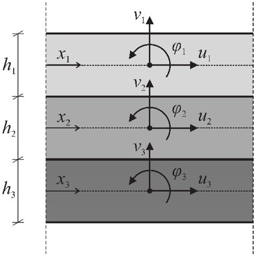
Kinematics of the beams: displacement components.

Equations (1)–(3), (4)–(6), and (7)–(9) represent the classical kinematic equations of the three linear beams (i = 1, 2, 3), while equations (10)–(13) represent the elongations of the normal (n) and the tangential (t) springs, respectively (subscript u stands for upper connecting layer, subscript d stands for bottom connecting layer).

It is worth observing that the length of the normal and tangential springs is not defined. Without losing generality, their length can be assumed as unitary. Therefore, the strains $ε_{nu}$ , $ε_{nd}$ , $ε_{tu}$ , and $ε_{td}$ can be formally considered as non-dimensional quantities.

Equilibrium equations

The equilibrium equations of the system refer to the internal stresses and the external forces shown in Figure 3 (left) and (right). They are obtained by equilibrating the internal stresses of each beam (N₁, V₁, M₁, N₂, V₂, M₂, N₃, V₃, M₃) and the stresses in the tangential and normal springs (τ_u, σ_u) and (τ_d, σ_d) with the external forces (see Figure 3 left and right). The equilibrium of internal stresses and external forces acting on the three infinitesimal portions of the coupled beams reads:

- N'_{1} - τ_{u} = 0

(14)

- V'_{1} - σ_{u} = P_{n 1}

(15)

- M'_{1} - V_{1} - \frac{h_{1}}{2} τ_{u} = 0

(16)

- N'_{2} - τ_{d} + τ_{u} = 0

(17)

- V'_{2} + σ_{u} - σ_{d} = P_{n 2}

(18)

- M'_{2} - V_{2} - \frac{h_{2}}{2} (τ_{u} + τ_{d}) = 0

(19)

- N'_{3} + τ_{d} = 0

(20)

- V'_{3} + σ_{d} = P_{n 3}

(21)

- M'_{3} - V_{3} - \frac{h_{3}}{2} τ_{d} = 0

(22)

Figure 3.

Statics of the beams: (left) internal stresses and (right) external forces.

where the external forces P_ni with (i = 1, 2, 3) account for the self-weight of layers.

Equations (14)–(16) represent the equilibrium of the forces in the tangential direction, in the normal direction, and of the moments respectively, acting on an infinitesimal portion of the upper beam#1; equations (17)–(19) represent the equilibrium of the forces in the tangential direction, in the normal direction and of the moments respectively, acting on an infinitesimal portion of the middle beam#2; equations (20)–(22) represent the equilibrium of the forces in the tangential direction, in the normal direction and of the moments respectively, acting on an infinitesimal portion of the bottom beam#3.

The three sets of three equations (equations (14)–(16), (17)–(19), and (20)–(22)) are coupled by the terms τ_u, τ_d, and σ_u, σ_d which are the tangential and normal stresses of the springs in the upper and lower position. As expected, the kinematic problem is the adjunct of the equilibrium problem.

Simplifications and assumptions

Some internal constraints were introduced following some suitable assumptions on the kinematical behavior of the mechanical system. Consequently, the mathematical problem can be simplified. However, for the cases under study, it is expected that the introduction of these constraints still makes the equations capable of well describing the mechanical behavior of the system.

The first internal constraint considered is the axial non-deformability of the middle beam:

ε_{2} = 0 \to u'_{2} = 0 \to u_{2} = k

(23)

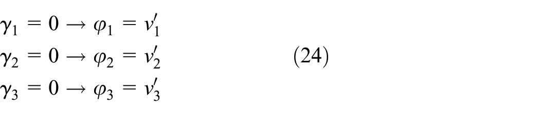
By taking into account the symmetry of the system, it was assumed that the constant value $k = 0$ and so $u_{2} = 0$ . It is worth observing that this constraint arises from the fact that the middle beam manifests an axial strain on average zero over the depth.

Then, the classical shear non-deformability of the beams was introduced. It leads to vanishing of the shear strains γ₁, γ₂, γ₃. Specifically, it reads:

\begin{matrix} γ_{1} = 0 \to φ_{1} = v'_{1} \\ γ_{2} = 0 \to φ_{2} = v'_{2} \\ γ_{3} = 0 \to φ_{3} = v'_{3} \end{matrix}

(24)

The last internal constraint is the infinite stiffness of the springs in the direction normal to the axis of the layers, representing the connection between the overlapping layers. This constraint has been introduced to simulate the impossibility of the fibers to detach from the timber surface of boards in the normal direction, and it leads to the vanishing of strains ε_nu and ε_nd, so that:

\begin{matrix} ε_{nu} = 0 \to v_{1} = v_{2} \\ ε_{nd} = 0 \to v_{3} = v_{2} \end{matrix}

(25)

By taking into account the equations (23)–(25), and imposing the same depth of the layers h₁=h₂=h₃=h, the kinematic equations equations (1)–(13), become:

\begin{matrix} ε_{1} = u'_{1} \\ ε_{3} = u'_{3} \\ κ_{1} = v''_{2} \\ κ_{2} = v''_{2} \\ κ_{3} = v''_{2} \\ ε_{tu} = u_{1} + h v'_{2} \\ ε_{td} = - u_{3} + h v'_{2} \end{matrix}

(26)

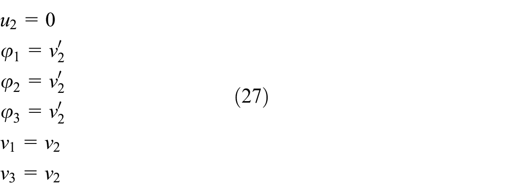
with internal constraint conditions:

\begin{matrix} u_{2} = 0 \\ φ_{1} = v'_{2} \\ φ_{2} = v'_{2} \\ φ_{3} = v'_{2} \\ v_{1} = v_{2} \\ v_{3} = v_{2} \end{matrix}

(27)

Due to the internal constraints, some internal forces (N₂, V₁, V₂, V₃, σ_u, σ_d) become reactive quantities. By condensing the equilibrium equations (14)–(22), they finally become:

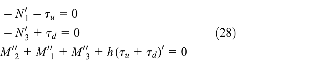
\begin{matrix} - N'_{1} - τ_{u} = 0 \\ - N'_{3} + τ_{d} = 0 \\ M''_{2} + M''_{1} + M''_{3} + h (τ_{u} + τ_{d})' = 0 \end{matrix}

(28)

with the reactive quantities:

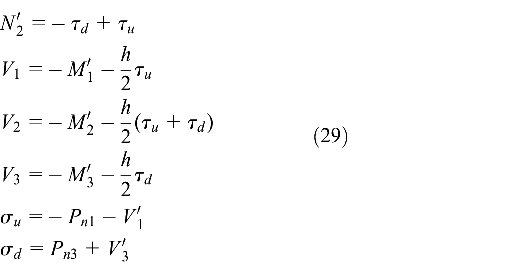
\begin{matrix} N'_{2} = - τ_{d} + τ_{u} \\ V_{1} = - M'_{1} - \frac{h}{2} τ_{u} \\ V_{2} = - M'_{2} - \frac{h}{2} (τ_{u} + τ_{d}) \\ V_{3} = - M'_{3} - \frac{h}{2} τ_{d} \\ σ_{u} = - P_{n 1} - V'_{1} \\ σ_{d} = P_{n 3} + V'_{3} \end{matrix}

(29)

where the distributed loads are neglected since they are small with respect to the forces applied during the experimental test.

Constitutive law

Supposing a linear elastic behavior for timber and connection springs, the constitutive laws were written as:

\begin{matrix} {\begin{matrix} N_{1} \\ N_{3} \\ M_{1} \\ M_{2} \\ M_{3} \\ τ_{u} \\ τ_{d} \end{matrix}} = [\begin{matrix} E_{1} A & 0 & 0 & 0 & 0 & 0 & 0 \\ 0 & E_{3} A & 0 & 0 & 0 & 0 & 0 \\ 0 & 0 & E_{1} I & 0 & 0 & 0 & 0 \\ 0 & 0 & 0 & E_{2} I & 0 & 0 & 0 \\ 0 & 0 & 0 & 0 & E_{3} I & 0 & 0 \\ 0 & 0 & 0 & 0 & 0 & g_{u} & 0 \\ 0 & 0 & 0 & 0 & 0 & 0 & g_{d} \end{matrix}] & {\begin{matrix} \begin{matrix} ε_{1} \\ ε_{3} \end{matrix} \\ \begin{matrix} κ_{1} \\ κ_{2} \end{matrix} \\ κ_{3} \\ ε_{tu} \\ ε_{td} \end{matrix}} \end{matrix}

(30)

Where E_i (i = 1, 2, 3) are the Young’s moduli of the three layers, g_u and g_d are the stiffnesses of the tangential springs representing respectively the upper and lower connections between the timber layers.

The field equations were obtained by accounting for the kinematic equation (26) in the constitutive laws (30) and then replacing them in the equilibrium equation (28). They read:

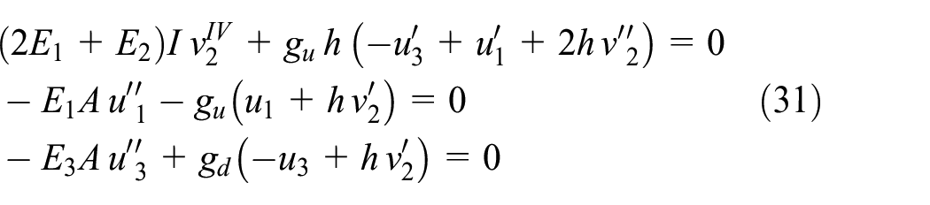
\begin{matrix} (2 E_{1} + E_{2}) I v_{2}^{IV} + g_{u} h (- u'_{3} + u'_{1} + 2 h v''_{2}) = 0 \\ - E_{1} A u''_{1} - g_{u} (u_{1} + h v'_{2}) = 0 \\ - E_{3} A u''_{3} + g_{d} (- u_{3} + h v'_{2}) = 0 \end{matrix}

(31)

where it was assumed that the upper and lower layer are realized with the same material (E₁ = E₃) and that the tangential springs have the same stiffness (g_u = g_d).

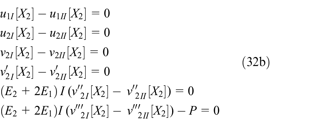
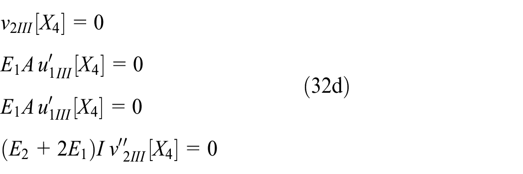
With reference to Figure 4, the boundary conditions for a simply supported beam with two concentrated loads symmetrically applied, read:

\begin{matrix} u_{1 I} [X_{1}] = 0 \\ u_{3 I} [X_{1}] = 0 \\ {v_{2}}_{I} [X_{1}] = 0 \\ (E_{2} + 2 E_{1}) I v' {'_{2}}_{I} [X_{1}] = 0 \end{matrix}

(32a)

\begin{matrix} u_{1 I} [X_{2}] - u_{1 II} [X_{2}] = 0 \\ u_{2 I} [X_{2}] - u_{2 II} [X_{2}] = 0 \\ v_{2 I} [X_{2}] - v_{2 II} [X_{2}] = 0 \\ v {'_{2}}_{I} [X_{2}] - v {'_{2}}_{II} [X_{2}] = 0 \\ (E_{2} + 2 E_{1}) I (v' {'_{2}}_{I} [X_{2}] - v' {'_{2}}_{II} [X_{2}]) = 0 \\ (E_{2} + 2 E_{1}) I (v ″ {'_{2}}_{I} [X_{2}] - v ″ {'_{2}}_{II} [X_{2}]) - P = 0 \end{matrix}

(32b)

\begin{matrix} {u_{1}}_{II} [X_{3}] - {u_{1}}_{III} [X_{3}] = 0 \\ {u_{3}}_{II} [X_{3}] - u_{3 III} [X_{3}] = 0 \\ v_{2 II} [X_{3}] - v_{2 III} [X_{3}] = 0 \\ v {'_{2}}_{II} [X_{3}] - v'_{2 III} [X_{3}] = 0 \\ (E_{2} + 2 E_{1}) I (v''_{2 II} [X_{3}] - v''_{2 III} [X_{3}]) = 0 \\ (E_{2} + 2 E_{1}) I (v ″'_{2 II} [X_{3}] - v ″'_{2 III} [X_{3}]) - P = 0 \end{matrix}

(32c)

\begin{matrix} v_{2 III} [X_{4}] = 0 \\ E_{1} A u {'_{1}}_{III} [X_{4}] = 0 \\ E_{1} A u'_{1 III} [X_{4}] = 0 \\ (E_{2} + 2 E_{1}) I v''_{2 III} [X_{4}] = 0 \end{matrix}

(32d)

Figure 4.

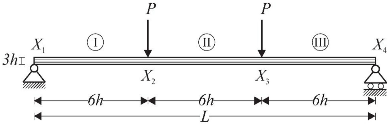
Four point bending scheme.

Due to the loading conditions, the beams are divided into three parts identified with Roman numbers from I to III (see Figure 4). Displacements with the subscripts I, II, and III refer to the part of the beam named with such Roman numbers. Equations (32a) and (32d) are the boundary conditions at X₁ and X₄, respectively; equations (32b) and (32c) are the boundary conditions at X₂ and X₃, respectively.

Approximate solution of the analytical system

The coupled system of three homogeneous differential equations (equation (31)), together with the boundary conditions (equations (32a)–(32d)), was solved by applying the Galerkin procedure. It is assumed that the unknown displacements u₁, u₃, and v₂ can be expressed as a linear combination of known shape functions Ψ_k(x) and Φ_k(x) and unknown coefficients α_k, β_k, and γ_k, as shown below:

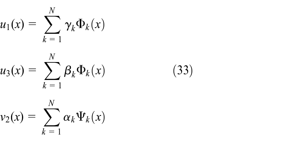
\begin{matrix} u_{1} (x) = \sum_{k = 1}^{N} γ_{k} Φ_{k} (x) \\ u_{3} (x) = \sum_{k = 1}^{N} β_{k} Φ_{k} (x) \\ v_{2} (x) = \sum_{k = 1}^{N} α_{k} Ψ_{k} (x) \end{matrix}

(33)

The known functions Ψ_k(x) and Φ_k(x) are Ψ_k(x)=Sin [(2k − 1)πx/L] and Φ_k(x) = Cos [(2k − 1)πx/L], with (k = 1, 2, … , N), respectively. They are chosen in such a way to select always the anti-symmetric Sine functions and the symmetric Cosine functions. Since they are continuous functions over the domain of the beam, only the boundary conditions at X₁ (the left boundary of the beam) and X₄ (the right boundary of the beam) have to be imposed. However, the chosen shape functions Ψ_k(x) and Φ_k(x) can satisfy identically the boundary conditions in equations (32a) and (32d). The presence of the two forces P applied at X₂ and X₃ was considered by computing the external virtual work done by these forces. The unknown coefficients α_k, β_k, and γ_k were obtained using the virtual work principle, whose equation reads:

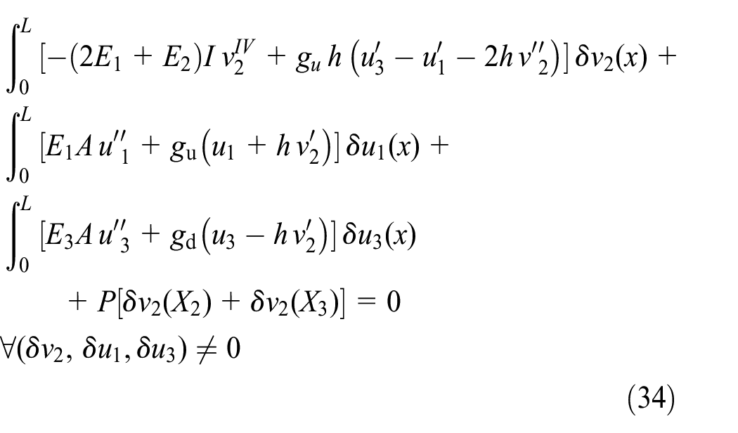
\begin{matrix} \int_{0}^{L} [- (2 E_{1} + E_{2}) I v_{2}^{IV} + g_{u} h (u'_{3} - u'_{1} - 2 h v''_{2})] δ v_{2} (x) + \\ \int_{0}^{L} [E_{1} A u''_{1} + g_{u} (u_{1} + h v'_{2})] δ u_{1} (x) + \\ \int_{0}^{L} [E_{3} A u''_{3} + g_{d} (u_{3} - h v'_{2})] δ u_{3} (x) \\ + P [δ v_{2} (X_{2}) + δ v_{2} (X_{3})] = 0 \\ \forall (δ v_{2}, δ u_{1}, δ u_{3}) \neq 0 \end{matrix}

(34)

where the equations inside the square brackets of the first three integrals are the equilibrium equations expressed as a function of the three unknown displacements (equation (31)) and the term $P [δ v_{2} (X_{2}) + δ v_{2} (X_{3})]$ accounts for the virtual work done by the two forces P. The virtual displacements δu₁, δu₃, and δv₂ read:

\begin{matrix} δ u_{1} (x) = \sum_{k = 1}^{N} δ γ_{k} Φ_{k} (x) \\ δ u_{3} (x) = \sum_{k = 1}^{N} δ β_{k} Φ_{k} (x) \\ δ v_{2} (x) = \sum_{k = 1}^{N} δ α_{k} Ψ_{k} (x) \end{matrix}

(35)

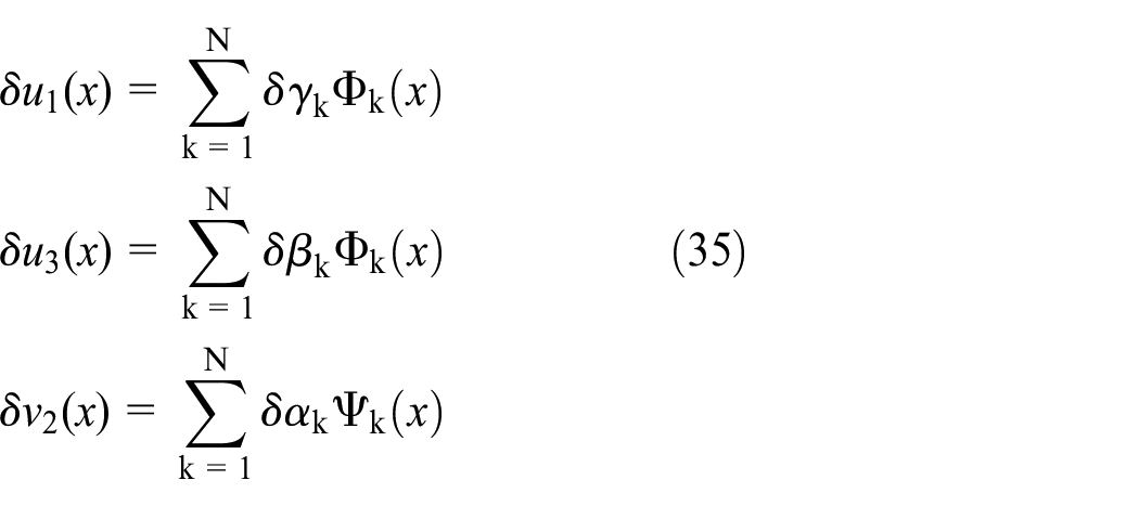
Expressing the displacements by equation (33) and the virtual displacement by equation (35), the virtual work equation (34) have to be satisfied ∀(δα_k, δβ_k, δγ_k) ≠ 0. By vanishing separately the terms multiplied to δα_k, δβ _k , δγ _k it is possible to obtain 3N algebraic equations, in the 3N unknown coefficients α_k, β_k, γ_k, that solved provides the values of α_k, β_k, γ_k. Once introduced into equation (33), these values can provide, in an approximate way, the unknown displacements. It is obvious that the greater the number of shape functions N, the better the approximation of the displacements.

Experiments

Two series of three-layered CLT panels were tested under out-of-plane four-point bending, in accordance with BS EN 16351 (2021) and UNI EN 408 (2010a). The tests were carried out in the testing laboratory of Materials and Structures (L.P.M.S.) of the University of L’Aquila. The first series of panels were made with Calabrian Beech (named homogeneous configuration), while the second one was made with Calabrian Beech (the outer layers) and Italian Corsican Pine (the inner layer) (named mixed configuration), see Figure 5. For each configuration, seven specimens were produced and tested (Sciomenta et al., 2020).

Figure 5.

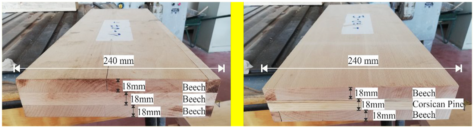
Xlam panels: (left) homogeneous configuration and (right) mixed configuration.

The geometrical properties, for both the homogeneous and mixed configurations, were defined following the BS EN 16351 (2021) and UNI EN 408 (2010a) for panels having a ratio of width b to depth h of b/h ≥ 4, the total length L was 21.85h and the length between the supports L_span was 18h. The main geometrical features were: the depth of each layer h₁ = h₂ = h₃ = 18 mm, the total panel depth h = 54 mm, the panel width B = 240 mm, the total length L = 1180 mm, and the distance of supports L_span = 972 mm.

The selected adhesive was a bi-component melamine glue (AkzoNobel—GripPro™ Design A002 (resin) and H002 (hardener)), specifically formulated for softwood and Beech, Chestnut, Birch, and Oak hardwood.

The Beech and Corsican Pine boards were graded visually (following UNI 11035 (2010b)) as by machine; this operation provided useful information about density, dynamic MOE, as well as moisture content, the results are summarized in Table 1. The global MOE of Beech and Corsican Pine was evaluated by previously formulated regression curves (Nocetti et al., 2010).

Table 1.

Main characteristics of the graded Beech and Corsican Pine boards.

Species	ρ_mean (kg/m³)	M.C. (%)	MOE_dyn (MPa)	MOE_gl (MPa)
Beech	754	9.5	16,482	15,933
Corsican Pine	499	13	8438	8408

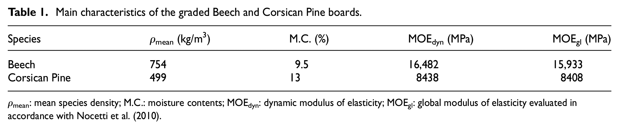
ρ_mean: mean species density; M.C.: moisture contents; MOE_dyn: dynamic modulus of elasticity; MOE_gl: global modulus of elasticity evaluated in accordance with Nocetti et al. (2010).

The elastic modulus of Beech and Corsican Pine was estimated following the boards’ machine grading based on the classification proposed by the EN 14081-2 (2018b) Table 2. The Beech was classified ad D40 class (E_m,0,mean=13,000 MPa, E_m,90,mean=870 MPa) and the Corsican Pine was C20 class (E_m,0,mean= 9500 MPa, E_m,90,mean = 320 MPa).

Table 2.

Elastic modulus assumed from the classification based on EN 338 (CEN, 2016).

Configuration	E_1,0,mean (MPa)	E_2,0,mean (MPa)	E_3,0,mean (MPa)
Homogeneous	13,000	870	13,000
Mixed	13,000	320	13,000

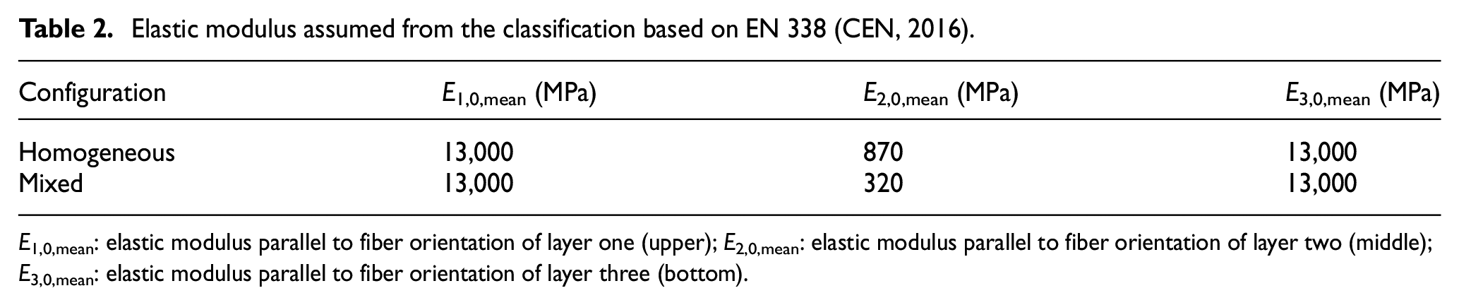
E_1,0,mean: elastic modulus parallel to fiber orientation of layer one (upper); E_2,0,mean: elastic modulus parallel to fiber orientation of layer two (middle); E_3,0,mean: elastic modulus parallel to fiber orientation of layer three (bottom).

Test methods

The simply supported specimens were symmetrically loaded in bending at two points over a span of 18 times the depth (Figure 6). To prevent the local indentation, two small steel plates were inserted between the specimens and the loading heads points (Figure 7).

Figure 6.

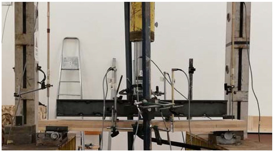
Experimental test setup.

Figure 7.

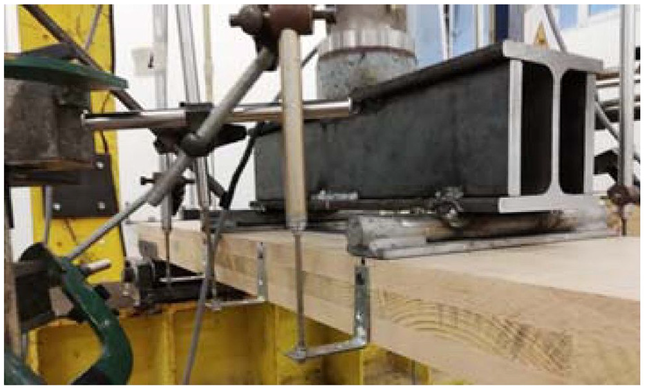
Plate detail.

The out-plane bending tests were performed up to failure, which occurred for a force level defined as F_max; an elastic behavior was accounted for up to 40% F_max. For each specimen, when the force level of 40% F_max was reached, the deflections were recorded in five different points, respectively: at the supports, at the loading heads points, and at mid-span.

The most common failure mechanism detected was the rolling shear, due to the low rolling shear stiffness of timber. Rolling shear fractures occurred at the ends of the beam portions, between the support area and the load application points; this mechanism was evident both for homogeneous as well as for mixed configurations as shown in Figure 8 left and right respectively.

Figure 8.

Rolling shear failures: (left) homogeneous and (right) mixed configuration.

Test results

The specimens having homogeneous configuration reached a 40% F_max level of 24.54 kN, which is 28% higher than for the mixed configuration; obviously, also the mean deflections estimated at the middle of the homogeneous configuration are 24% higher compared to that measured for the mixed configuration (Figures 9 and 10).

Figure 9.

Out-plane bending test BS EN 16351 (CEN, 2021) UNI EN 408 (UNI, 2010a) for homogeneous configuration: (left) deflections and (right) forces.

Figure 10.

Out-plane bending test BS EN 16351 (CEN, 2021) UNI EN 408 (UNI, 2010a) for mixed: (left) deflections and (right) forces.

Comparison among experimental and analytical results

The values defined in Table 2 were assumed in the analytical formulation for timber layers’ mechanical properties. The elastic moduli of the upper and lower beams are increased by dividing them by the coefficient $1 - ν^{2}$ ( $ν = 0.3$ ), to take into account the plate effects due to the Poisson coefficient. The melamine glue has a tangential stiffness G = 642 MPa (de Oliveira et al., 2018). Adhesive layers were modeled as elastic springs in the 1D formulation; these springs have a tangential stiffness g_u = g_d = G·B, where B is the panel’s width. In Figure 11, the deflections evaluated by using the proposed model are compared with those obtained from the test. In both homogeneous and mixed configurations, as shown, the correspondence is rather good, but the analytical models generally tend to underestimate the experimental ones.This fact occurs since the model is a bit stiffer than the real case, due to the internal shear rigidity. However, the small differences between the deflections provided by the model and the experimental test, shows that the shear rigidity plays a marginal role.

Figure 11.

Deflection comparison between the novel analytical formulation and the experimental tests.

The analytical model was capable to account for the tangential stress at the interface between the timber-to-glue layers. As it is evident in Figures 12 and 13, there is an extremely higher tension level on the beam’s edges (in particular from the point of application of loads up to the ends of the beam). This clarifies the reason for the activation of the rolling shear mechanism in these particular regions of the panel. Such tangential stress is negligible between the two loads, where the shear is constant and maximum. To highlight the good convergence of the approximate solution toward the true one, in Figures 12 and 13 the tangential stress is plotted by increasing the number of shape functions.

Figure 12.

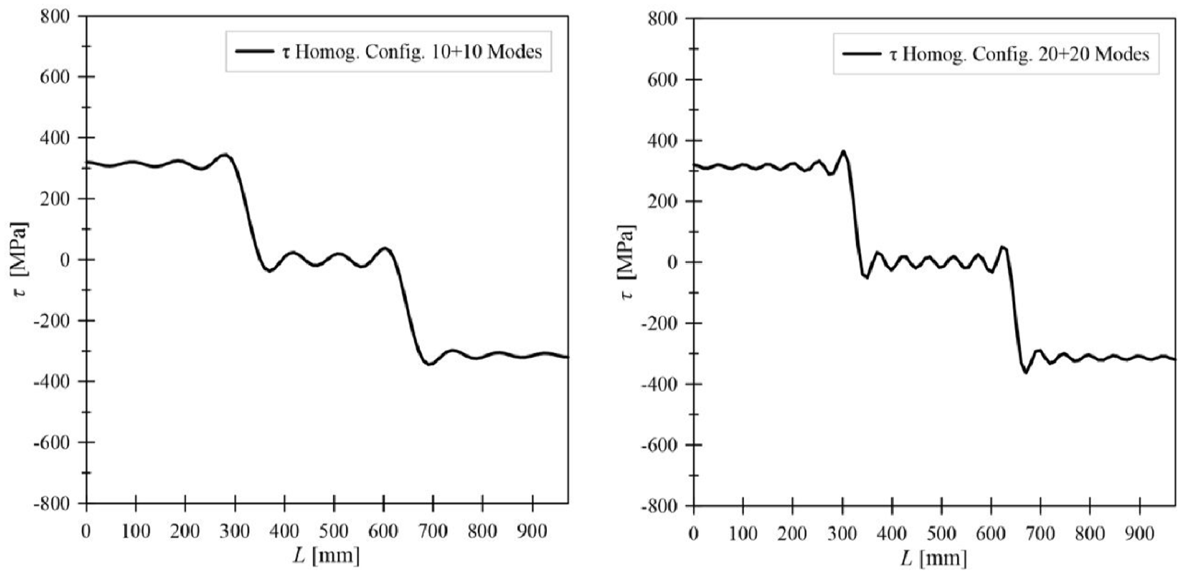
Tangential stress estimated at the interface between glue and timber layer for the homogeneous configuration: (left) 10 modes and (right) 20 modes.

Figure 13.

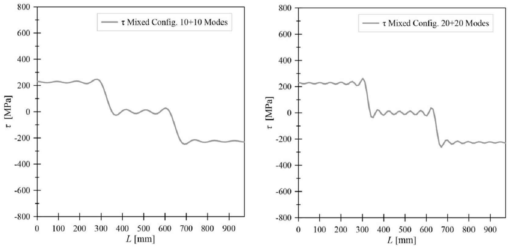
Tangential stress estimated at the interface between glue and timber layer for the mixed configuration: (left) 10 modes and (right) 20 modes.

Literature’s method

Assumptions

The literature’s method adopted for the evaluation of the stress values and deflections is the γ-method (adopted in Eurocode 5 (2010)) and the K-method (Blass and Fellmoser, 2004) (see Subsection 1.2). Those methods do not account for the shear deformability, contrary to the Shear Analogy method, so their results can be directly compared with those obtained from the purposed analytical formulation. The three-layered panel stiffness K_Clt was evaluated according to the Eurocode 5 (2010) in the γ-method and according to the Blass and Fellmoser (2004) formulation in the K-method. The deflection f was evaluated considering the Euler-Bernoulli beam relationship. In Table 3 the main parameters evaluated with the previous methods and via experimental test are summarized.

Table 3.

Licterature’s method and experimental parameters.

	Geometric parameters			Experimental			γ-method						K-method
Configurationtype	h (mm)	b (mm)	l (mm)	K_Clt(kNm²)	F (kN)	f (mm)	γ₁	γ₃	K_Clt(kNm²)	F (kN)	f (mm)	k ₁	K_Clt (kNm²)	F (kN)	f (mm)
Homogeneous	54	240	1180	43.3	18.9	9.4	0.65	1.0	31.7	15.9	16.4	0.97	39.53	19.9	16.4
Hybrid	54	240	1180	46.3	14.2	7.1	0.65	1.0	29.5	14.8	16.4	0.96	39.46	19.8	16.4

γ_i is the composition coefficient of ith layer; k₁ is the composition factor which depends on the type and direction of an external force acting on the panel.

Results

The results provided from the application of these two methods are displayed in Figure 14 (left) for homogeneous configuration and (right) for mixed configuration. As highlighted in Figure 14, the Experimental values of force measured during tests (and adopted for the analytical evaluations) is, in both cases, underestimated by the γ-Method; if the K-Method is adopted, the calculated force is close to the experimental one but it is underestimated in the homogeneous configuration and overestimated in the mixed configuration case. In terms of flexural deflection of the middle point of the panel, the γ-Method and the K-Method (green dots) markedly overestimate the experimental value (red dot). On the contrary, the analytical model provides a deflection (blue dot) in good agreement with the experimental one.

Figure 14.

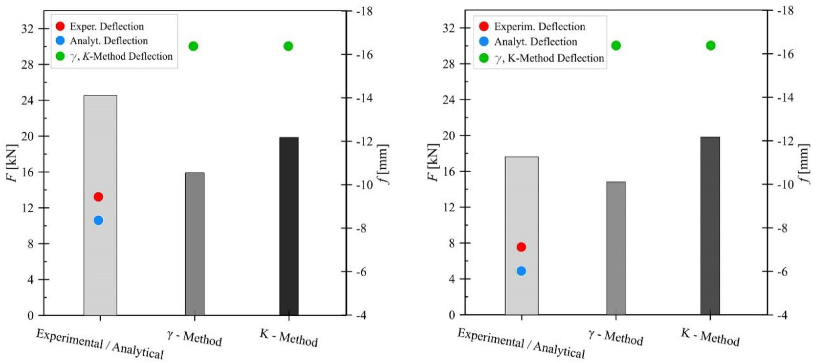
Forces and deflections evaluated via analytical methods for: (left) homogeneous configuration and (right) mixed configuration.

Finite element analysis

Key assumptions and boundary conditions previously defined in the analytical and experimental analyses were further assessed with the support of parametric Finite Element (FE) investigations. The numerical simulations were carried out by using the ABAQUS/Explicit software package (Dassault Systèmes Simulia, 2015), in the form of quasi-static imposed force history for the CLT panels in Figure 15.

Figure 15.

Finite Element modeling of a panel.

The Explicit solver was chosen to facilitate the convergence of simulations, given that a series of contact interactions were used at the CLT interfaces. The typical model was developed to represent all the specimens’ components (wood and glue). A set of 8-node 3D solid elements, C3D8R-type stress-strain bricks with reduced integration, was used, as available in the ABAQUS library. Rigid base support was also described via C3D8R-type, 3D solid elements, to schematically reproduce the testing machine (loading region and end supports) and the related effects (i.e. contact between the base surface and the circular section representative of the hinge support), see Figure 16.

Figure 16.

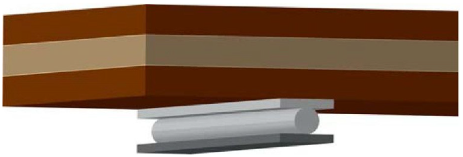
Finite element modeling of pinned support (detail).

Two different approaches were proposed in this work (Figure 17):

Figure 17.

Scheme of FE models in accordance with: Approach 1 (left) and Approach 2 (right).

Approach 1: The porous nature of wood was fully neglected, and the timber layers were modeled assuming the mechanical features in Table 4 with layers of glue between them.

Approach 2: The wood porous nature was taken into account. As such, a fraction of glue was considered absorbed into the wood layers, and another fraction of glue was accounted to describe a thin layer interposed between the timber boards. Layers were modeled assuming the mechanical features in Table 4.

Table 4.

Elastic and shear modulus of Beech D40, Black Pine C20, and “Approach 2” layers.

Panel configuration	Glue configuration	θ = 0°			θ = 90°			θ = 0°
		E_1,0,mean(MPa)	E_1,90,mean(MPa)	G_1,mean(MPa)	E_2,0,mean(MPa)	E_2,90,mean(MPa)	G_2,mean(MPa)	E_3,0,mean(MPa)	E_3,90,mean(MPa)	G_3,mean(MPa)
Homogeneous	Approach 1. 1 mm/3 mm	13,000	870	810	13,000	870	810	13,000	870	810
	Approach 2.1 mm	12,958	873	809	12,958	873	809	12,958	873	809
	Approach 2. 3 mm	12,876	880	808	12,876	880	808	12,876	880	808
Mixed	Approach 1. 1 mm/3 mm	13,000	870	810	9500	320	590	13,000	870	810
	Approach 2.1 mm	11,796	691	736	11,796	691	736	11,796	691	736
	Approach 2. 3 mm	11,723	699	735	11,723	699	735	11,723	699	735

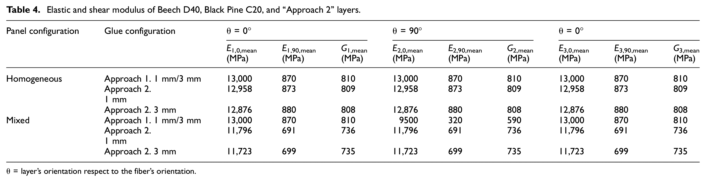
θ = layer’s orientation respect to the fiber’s orientation.

Two different glue thicknesses were assumed: 0.1 and 0.3 mm, which represent respectively the minimum and the maximum limit for the adhesive depth suggested in the technical datasheet.

The melamine glue was considered as an isotropic elastic material having E=1800 MPa, G=642 MPa, and ν=0.4 (de Oliveira et al., 2018). An isotropic, elastic Von Mises constitutive law was defined for the steel plates and tubes by accounting for E = 210 GPa and ν = 0.3 as nominal MOE and Poisson’ ratio. Regarding timber, Beech was mechanically characterized according to Table 2 (that is D40 class), while Corsican pine was classified as C20.

For Approach 2, following de Oliveira et al. (2018), the method of the transformed section was adopted to predict the mechanical properties of layers composed of wood and glue, which are summarized in Table 4. This operation allows the user to define a layer having “homogenized” elastic and shear modulus.

A key role was finally assigned to mechanical contacts and interactions for the so described FE components, to reproduce the actual behavior of test specimens under investigation. Given the reference FE assembly, tangential “penalty” and normal “hard” surface-to-surface behaviors were first defined for the steel-to-timber surfaces in contact, to account for the relative slip during the overall loading phase. There, the static friction coefficient was set equal to μ = 0.2 according to Bedon and Fragiacomo (2019). A similar surface-to-surface contact interaction (with μ = 0.2 the corresponding friction coefficient (Zhang et al., 2008)) was then assigned to the interface between the steel support plate and the steel tube, representative of the pinned joint. Each timber layer and the overlapped glue layer were then rigidly connected via a “tie” mechanical constraint.

The quasi-static incremental loads were applied as two concentrated forces acting on each upper plate. These latter were adopted to distribute the load along a line, avoiding the panel’s plasticization due to compression loads perpendicular to the fiber orientation.

FE results and comparisons

In Figure 18 (left)–(right), the deflection curves for the homogeneous and mixed configurations (and for the glue layer of 0.1 and 0.3 mm) are shown. In both the homogeneous and mixed configurations, the increase of adhesive thickness involves slightly higher flexibility (0.12% and 2.1% respectively). Moreover, for the homogeneous configuration, the models carried out by adopting “homogenized” mechanical properties do not diverge from the solution obtained by modeling the glue layers. For the mixed configuration, the difference between the layered and the “homogenized” models is more evident (10%–16%). This difference is mainly due to the adoption of the transformed section method, which considers the composite made up of matrix and fibers; in our mixed configuration there is the simultaneous presence of two different timber species, so the homogenization technique led to less accurate results.

Figure 18.

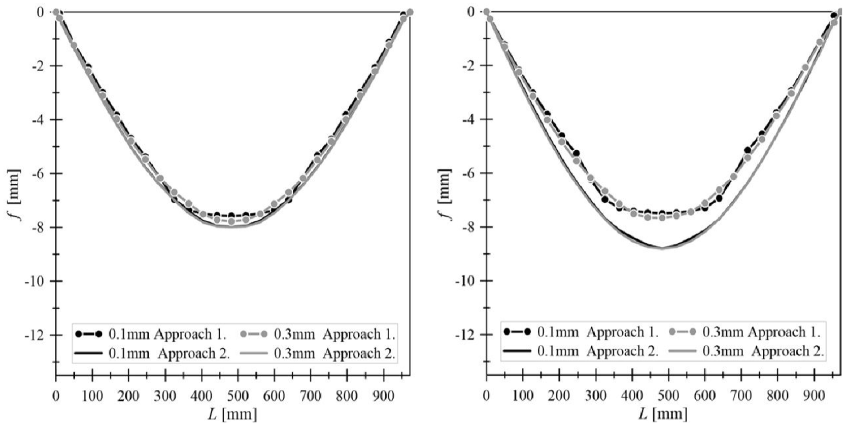
FE deflection curves: (left) homogeneous and (right) mixed configuration.

Finally, for each of the two examined configurations, a comparison between experimental, analytical, and FE deflection curves is provided (Figure 19). The FE results highlight an overall good accuracy related to experimental curves. In the homogeneous configuration, the analytical deflections differ from the experimental ones by +11%, while the discrepancy between the experimental deflections and the numerical ones is +15%. In the mixed configuration, the experimental deflections and the analytical ones diverge at +15%, while the difference between the experimental deflections and the numerical ones is −22%.

Figure 19.

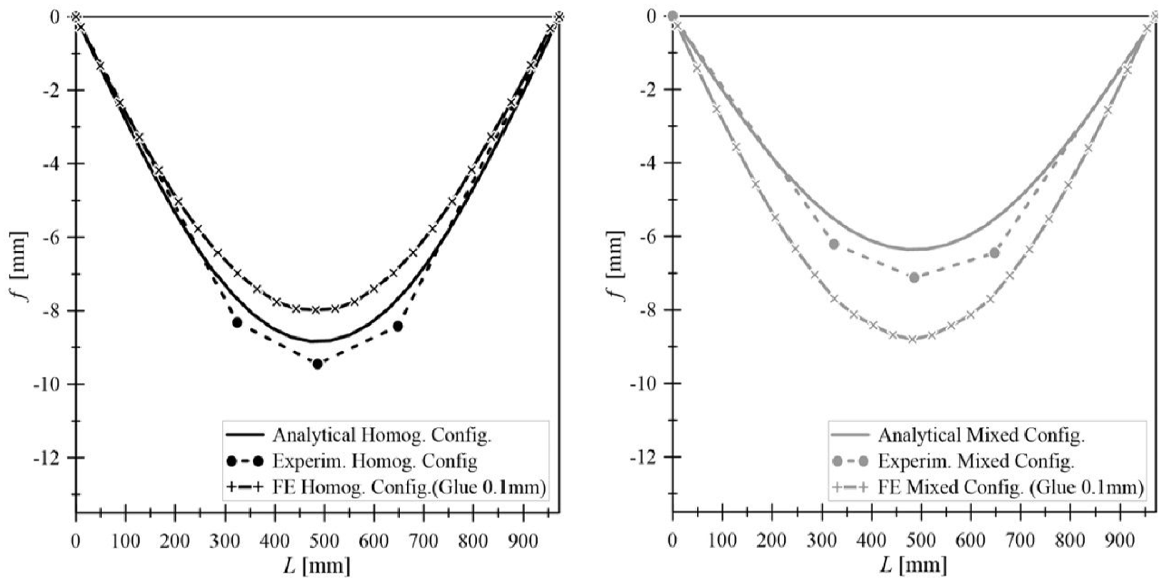
Experimental, analytical, and numerical deflection curves comparison: (left) homogeneous and (right) mixed configuration.

Conclusions

In this paper, the structural performance of two series of three-layered CLT timber panels was investigated via experimental, analytical, and FE analysis. The analytical and FE modeling assumptions were validated toward the experimental results. Comparative results were hence critically discussed in the paper, both for mixed and homogeneous specimen configurations.

The analytical model was formulated by mean of overlapped 1D beams connected via elastic devices which represent the glue layers. This quite simple model generally gave evidence of fairly close correlation with the reference experimental test results, both for the homogeneous specimens and the mixed ones. Moreover, this model was capable of predicting the tangential stress at the timber-to-adhesive interface, and so justifying the activation of the subsequent rolling shear mechanisms from the two load support points to the outside bounds, since the highest tangential stress occurs right between the loads’ points and the ends of the panel.

For the analytical results, in particular, an average scatter of +11% or +15% was observed respectively for the homogeneous and mixed configuration; in both cases, the analytical model slightly underestimates the deflection.

A good match was also found with the FE simulations; a 3D elastic model was formulated by accounting for the glue layers as well as adopting the transformed section method and performing a “homogenization” of elastic and shear modulus. For the homogeneous configuration, the deflection was underestimated by15% if compared with experimental one; for the mixed configuration, the numerical deflection was overestimated by 22%.

Footnotes

Declaration of conflicting interests

The author(s) declared no potential conflicts of interest with respect to the research, authorship, and/or publication of this article.

Funding

The author(s) disclosed receipt of the following financial support for the research, authorship, and/or publication of this article: The panels were realized courtesy of XlamDolomiti S.r.l. (Trento, Italy). The work was financially supported by the Ministry for Education, the University, and the Research, Grant: PRIN 2015 Prot. 2015YW8JWA entitled “The short supply chain for biomasses and timber: procurement, traceability, certification, and Carbon Dioxide sequestration. Innovation for the bio-architecture and energy efficiency.”

ORCID iDs

Angelo Di Egidio

Chiara Bedon

Massimo Fragiacomo

References

Bedon

Fragiacomo

(2019) Numerical analysis of timber-to-timber joints and composite beams with inclined self-tapping screws. Composite Structures 207: 13–28.

Blass

Fellmoser

(2004) Design of solid wood panels with cross layers Influence of shear deformation. In: Proceedings of the 8th world conference on timber engineering, WCTE 2004, Lahti, Finland, 14–17 June, pp.543–548.

Brandner

Tomasi

Thomas

, et al. (2018) Properties, Testing and Design of Cross Laminated Timber. A State of the Art Report by COST Action FP1402/WG 2. Aachen: Shaker Verlag.

CEN (European Committee for Standardization) (2010) Eurocode 5: Design of timber structures - Par 1-1: General - Common rules and rules for buildings. Brussels, Belgium. DOI: 10.1680/cien.2001.144.6.39.

CEN (European Committee for Standardization) (2016) Structural timber - Strength classes. EN 338. Brussels, Belgium.

CEN (European Committee for Standardization) (2018b) Timber Structures – Strength graded structural timber with rectangular cross-section – Part 2: Machine grading; additional requirements for type testing. EN 14081-2. Brussels, Belgium.

CEN (European Committee for Standardization) (2021) Timber Structures - Cross laminated timber - Requirements. 16351. Brussels, Belgium.

Chirivì

Ibell

Contento

, et al. (2016) Linear static behavior of curved beams coupled with strings representing also fiber-reinforced masonry arches. Advances in Structural Engineering 19(1): 53–64.

Dassault Systèmes Simulia (2015) Abaqus F.E.A. v. 6.12 computer software. Providence, RI, USA.

10.

de Oliveira

SJC

Bolmin

Arrigoni

, et al. (2018) Plywood experimental investigation and modeling approach for static and dynamic structural applications. In: Advanced Structured Materials (Eds. Andreas Öchsner, Holm Altenbach). Springer, 2018, pp.119-141. Advanced Structured Materials book series.

11.

DIN (German Institute for Standardization) (2004) Design of timber structures – General rules and rules for buildings. DIN 1052: chapter 8.6.2.

12.

Kreuzinger

(1999a) Flächentragwerke - Platten, Scheiben und Schalen – Berechnungsmethoden und Beispiele. Fachverlag Holz. Düsseldorf, pp.43–60.

13.

Kreuzinger

(1999b) Platten, Scheiben und Schalen. Bauen mit Holz 101(1): 34–39.

14.

Kreuzinger

(2000) Verbundkonstruktionen aus nachgiebig miteinander verbundenen Querschnittsteilen. Ingenieurholzbau Karlsruher Tage. Karlsruhe, pp.43–55.

15.

Kreuzinger

(2002) Verbundkonstruktionen. Holzbaukalender. Karlsruhe, pp.598–621.

16.

Möhler

(1956) Über das Tragverhalten von Biegeträgern und Druckstäben mit zusammengesetztem Querschnitt und nachgiebigen Verbindungsmitteln. Thesys, Karlsruhe.

17.

Murakami

(1986) Laminated composite plate theory with improved in-plane responses. Journal of Applied Mechanics 53(3): 661–666.

18.

Nocetti

Bacher

Brunetti

, et al. (2010) Machine grading of Italian structural timber: preliminary results on different wood species. In: Proceedings WCTE 2010 - World conference on timber engineering, Trento, Italy, pp.1-7.

19.

Pagano

(1970) Exact solutions for rectangular bidirectional composites and sandwich plates. Journal of Composite Materials 4(1): 20–34.

20.

Ren

(1986) A new theory of laminated plate. Composites Science and Technology 26(3): 225–239.

21.

Sciomenta

Spera

Bedon

, et al. Mechanical Characterization of novel Homogeneous and Hybrid Beech-Corsican Pine Thin Cross-Laminated Timber Panels. Construction and Building Materials, 2020.

22.

Simoneschi

Di Egidio

de Leo

, et al. (2016) On the use of reinforcing layers to improve the static behaviour of arches or shells with single curvature. Advances in Structural Engineering 19(8): 1302–1312.

23.

Stürzenbecher

Hofstetter

Eberhardsteiner

(2010) Structural design of Cross Laminated Timber (CLT) by advanced plate theories. Composites Science and Technology 70(9): 1368–1379.

24.

UNI (Ente Nazionale Italiano di Unificazione) (2010a) EN 408:2010 - Timber structures - Structural timber and glued laminated timber: Determination of some physical and mechanical properties.

25.

UNI (Ente nazionale italiano di unificazione) (2010b) Legno strutturale - Classificazione a vista dei legnami secondo la resistenza meccanica [Structural wood - Visible classification of wood according to mechanical resistance]. UNI 11035.

26.

Zhang

Nagae

McCormick

, et al. (2008) Friction-based sliding between steel and steel, steel and concrete, and wood and stone. In: Proceedings of the 14th World Conference on Earthquake Engineering, Beijing, China.