



Abstract
For rail vehicles, the spanwise correlation of aerodynamic forces acting on a single car is usually overlooked. To investigate the effects of spanwise correlation functions on the dynamic responses of the rail vehicle-bridge coupling system, firstly, the forms of spanwise correlation functions in the aerodynamic forces of a running vehicle, which are associated with the longitudinal and vertical fluctuating wind speeds, were proposed. Secondly, the spectra of buffeting forces acting on the running vehicle considering those spanwise correlation functions were obtained. Thirdly, a rail vehicle-bridge coupling system was established by using the commercial software SIMPACK, and a single car running on a typical high-speed railway bridge was taken as an example. Again, the effects of artificial discrete wind fields on the dynamic responses of the vehicle and bridge were investigated. Finally, the effects of the above spanwise correlation functions on the dynamic responses of the rail vehicle-bridge coupling system were compared under the cases of different vehicle speeds and wind speeds. The results show that different discrete time intervals can exert significant effects on the vehicle responses, and the discrete time interval of 0.05 s can be used for analysis in the wind-rail vehicle-bridge coupling system. With the increase of vehicle speed, the values of vehicle and bridge responses considering the spanwise correlation functions tend to be close to those without considering the spanwise correlation functions. However, as the wind speed increases, the values of vehicle and bridge responses generally tend to show greater differences in the presence and absence of spanwise correlation functions. At different vehicle speeds or wind speeds, the spanwise correlation functions have significant effects on the RMSs of vehicle accelerations and bridge lateral acceleration, but they have little effects on the bridge vertical acceleration.
Keywords
Introduction
At present, there are up to 22,000 kilometers of high-speed railway in operation in China, accounting for about 65% of the total length in the world. It is estimated that a high-speed railway network of 38,000 kilometers will have been established in China by 2025 (The State Council Information Office, PRC 2016). In order to ensure the smooth and high-speed running of trains on the whole line, the proportion of the bridge in high-speed railway accounts for as high as over 50% on average. Besides, modern high-speed trains further develop towards higher speed and lighter weight, which thus become more and more sensitive to the action of winds. With the construction and operation of high-speed railway in coastal and inland strong wind areas in China, more attention should be paid to ensure high-speed trains running on bridges safely and smoothly under strong wind environments.
Accurate calculation of wind loads of the vehicle and bridge are the premise of the safety and comfort of high-speed trains running on bridges under strong wind environments. To this end, the aerodynamic forces of the vehicle and bridge should be separated, respectively, first in the study of coupling vibration of wind-rail vehicle-bridge system. Li et al. (2005); He and Li (2020) separated the static three-component forces of the vehicle and bridge with force measurement method based on wind-tunnel techniques, when the vehicle is stationary. Pressure measurement method is also effective for simple girder sections (Guo et al., 2015; He et al., 2014). In addition to the static three-component coefficients above, the aerodynamic admittance function of the vehicle and bridge should also be established for their unsteady buffeting forces. When the vehicle is stationary, there are no large differences between the aerodynamic admittance function test method of the vehicle and bridge and that of ordinary bluff bodies. Sterling et al. (2009) measured the aerodynamic admittance functions of various types of rail vehicles by wind tunnel test and field measurement methods, combined with force and pressure measurement techniques, and finally established an expression of aerodynamic admittance function for the side force and lift force of vehicles. Subsequently, Baker (2010) simplified the above expression of aerodynamic admittance function. Yan et al. (2018) tested the aerodynamic admittance function of a CRH vehicle under different wind direction angles in a wind tunnel, and suggested that the aerodynamic admittance functions of the side and lift forces of the vehicle could be approximately regarded as a constant within the dimensionless frequency range concern to the train. It should be noted that since stationary vehicles often fail to truly simulate the aerodynamic characteristics between running vehicles and bridges, it is necessary to develop a set of model test device for running vehicles based on wind tunnel tests. For instance, Baker (1986); Bocciolone et al. (2008); Howell (1986); He et al. (2014); Li et al. (2013); Xiang et al. (2017) have successively developed different types of model test devices for running vehicles in wind tunnels, which preliminarily revealed the variation rules of three-component coefficients of vehicles and bridges, and paved the way for the test and analysis of the aerodynamic admittance function of vehicles.
Based on the aerodynamic parameters above, Cooper (1984) obtained the spectra of side force of the running vehicle by assuming that the aerodynamic forces of the vehicle have a linear relationship with the longitudinal fluctuating wind speeds. Li et al. (2005) derived the buffeting force formulas of running vehicles with the effects of longitudinal and vertical fluctuating wind speeds both considered, in which the “cosine rule” (Chiu and Squire, 1992) was used to approximately consider the aerodynamic coefficients of running vehicles. Xu and Ding (2006) simulated the steady and unsteady aerodynamic forces on a rail vehicle, and the safety and comfort performance of the rail vehicle under crosswinds were discussed. Baker (2010) investigated the influences of longitudinal fluctuating wind speed on wind direction angles. Yu et al. (2016) studied the probability distribution characteristics of the unsteady aerodynamic loads on rail vehicles. Based on the research above, Yan et al. (2018) investigated the effects of longitudinal, lateral, and vertical fluctuating wind speeds on vehicles, thus making the aerodynamic forces of the vehicle more refined. However, for rail vehicles, it should be pointed out that every single car is relatively long, but the traditional commercial software and self-made programs for modeling the wind-rail vehicle-bridge coupling system usually only set one wind load point on a single car, which is equivalent to the fact that the aerodynamic forces along every single car are fully correlated. Obviously, the above traditional modeling method will result in overestimation of the wind loads acting on the vehicle, and the bridge responses will probably also be overestimated. For stationary vehicles, some studies combined the parameters of spanwise correlation and the aerodynamic admittance function of the vehicle, then the two different parameters become an equivalent parameter (Gisella and Cheli, 2013). However, for running vehicles, on the one hand, it is very hard to measure their aerodynamic admittance functions. On the other hand, the spanwise correlation, which is equivalent to a transfer function from fluctuating wind speed spectra to aerodynamic force spectra, is unknown. Therefore, it is difficult to accurately estimate the aerodynamic forces of such running vehicles in the atmospheric boundary layer, which will cause some errors in the dynamic response of rail vehicle-bridge coupling system subject to wind loads.
This study focuses on the spanwise correlation of aerodynamic forces acting on a single car and their effects on the dynamic responses of rail vehicle-bridge coupling system. First of all, the forms of spanwise correlation function in the aerodynamic forces of a running vehicle, which are associated with the longitudinal and vertical fluctuating wind speeds, were proposed. On such basis, the spectra of buffeting forces acting on the running vehicle considering the spanwise correlation functions were obtained according to the cosine rule. Then, a rail vehicle-bridge coupling system was established by using the commercial software SIMPACK, and a single car running on a typical high-speed railway bridge was taken as an example. The effects of the artificial discrete wind field on the responses of the vehicle and bridge were investigated, and the effects of the above spanwise correlation functions on the dynamic responses of the vehicle and bridge were compared under the cases of different vehicle speeds and different wind speeds. Finally, some main conclusions are presented.
Fluctuating wind speed spectra and fluctuating wind coherence function of running vehicles
According to Taylor hypothesis and homogeneous isotropic turbulence hypothesis, Cooper (1984); Li et al. (2017); Wu et al. (2014) have successively proposed an expression of fluctuating wind speed spectra for running vehicles. However, homogeneous isotropic turbulence hypothesis is not applicable to running vehicles in the atmospheric boundary layer. Based on the longitudinal Simiu spectra and Davenport coherence function in the wind-resistant specification of China (JTG/T 3360-01, 2018); Yan et al. (2018) and Hu et al. (2019) both proposed a new model of fluctuating wind speed spectra for running vehicles. Among them, Hu et al. (2019) also established a coherence function model of fluctuating wind speed for running vehicles. Besides, Hu et al. (2019) verified the fluctuating wind speed spectra and the coherence function model of fluctuating wind speed for running vehicles and proposed specific expression forms, which is convenient to use. Therefore, the expression proposed by Hu et al. (2019) is adopted in this paper. The spectra of longitudinal fluctuating wind speed relative to running vehicles, denoted by SuM(n), is expressed as follows

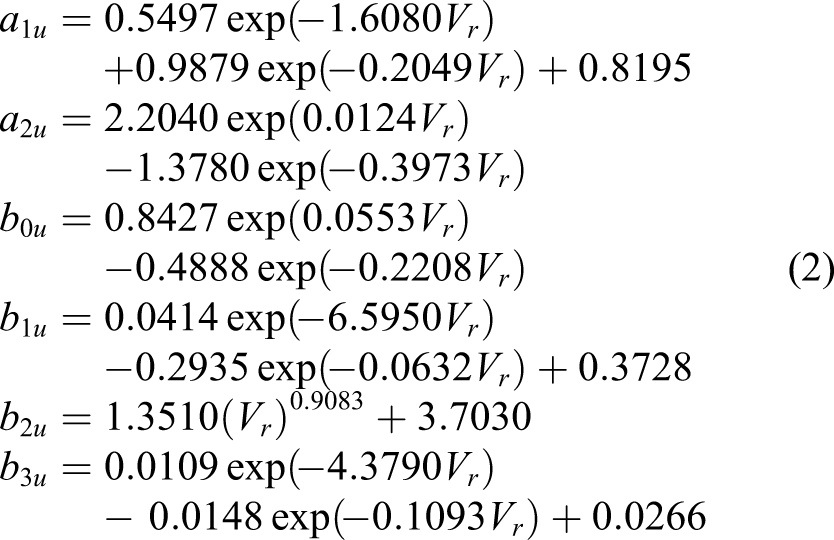
The expression of the coherence function of the longitudinal fluctuating wind speed relative to the running vehicle,

It should be noted that the coefficient α0 in equation (3) is a function of Vr, Δ and z, which is inconvenient to use since it involves many parameters. In order to investigate the sensitivity of the parameters Δ and z in the coefficient α0 to the value of The values of CohuM under different Δ values in the coefficient α0.
It should be noted that equation (3) is inconvenient for integral calculation. However, it can be seen from Figure 1 that the values of the coherence function Coh
uM
monotonically decrease with the values of the horizontal coordinate n · Δ/U. Obviously, this smooth curve could be easily fitted by a polynomial function. Based on the calculation results of equation (3), an 8-order polynomial function can be used to express the values of Coh
uM
as follows to facilitate the sub sequent integral calculation Comparison between the values calculated by equation (4) and those by the simplified form.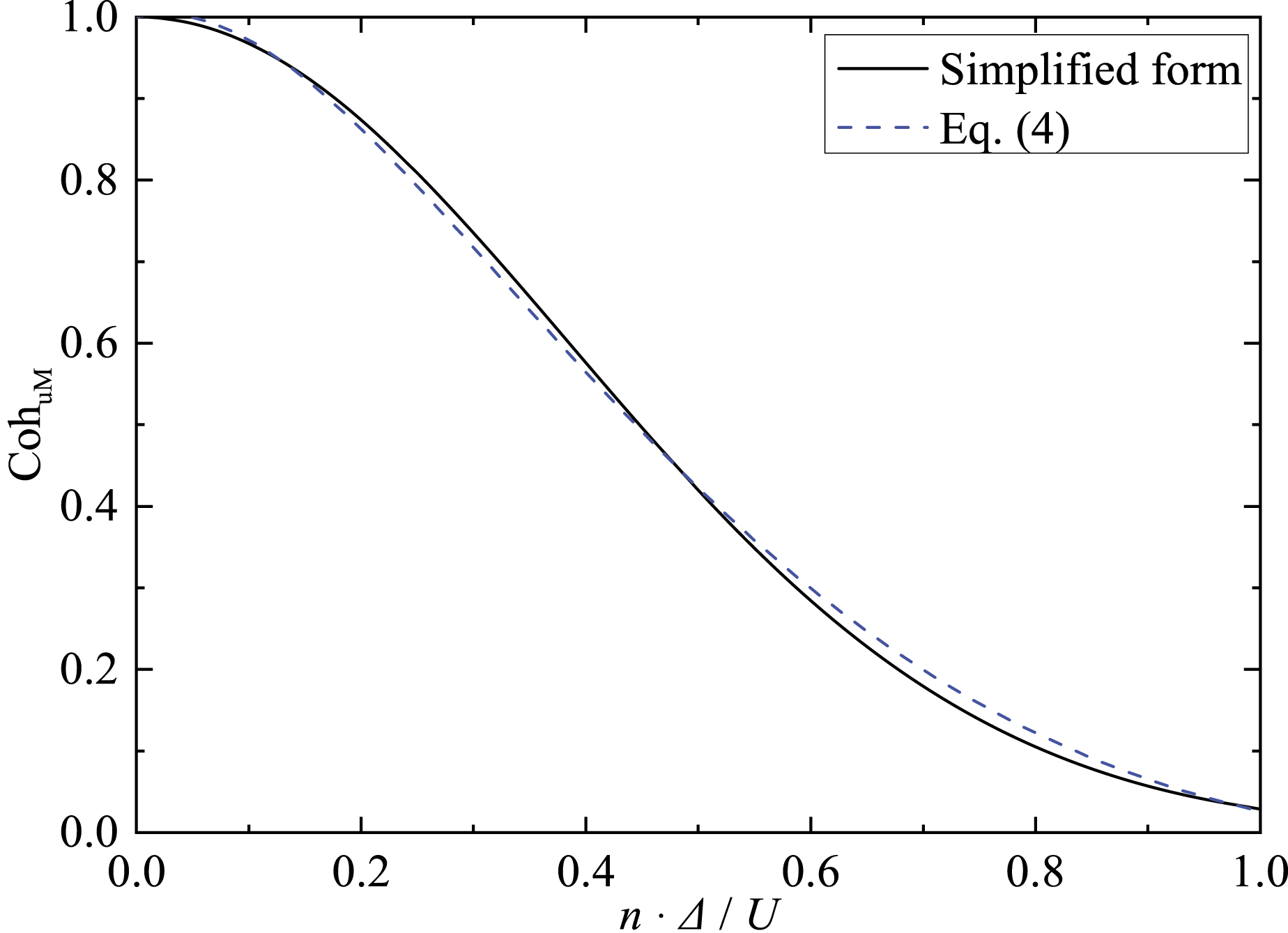




The spanwise correlation of aerodynamic forces relative to running vehicles
In previous studies on the coupling vibration of wind-rail vehicle-bridge systems, only one wind load point was set on each single car, which is equivalent to the assumption that the fluctuating wind speeds and wind loads along the car body is fully correlated, as shown in Figure 3(a). Actually, the fluctuating wind speeds and wind loads along the vehicle or a single car cannot be full correlated at any time period, as shown in Figure 3(b). The side force of the vehicle body caused by the longitudinal fluctuating wind speeds is taken as an example for analysis, so as to analyze the spanwise correlation of the aerodynamic forces of the running rail vehicle subsequently. Fluctuating wind speeds relative to a single car with different spanwise correlation. (a) Fully spanwise correlation; (b) Partially spanwise correlation.
According to the theory of quasi-steady state, assuming that “cosine rule” is applicable (Chiu and Squire, 1992; Li et al., 2005), the side force per unit length of the vehicle body caused by the longitudinal fluctuating wind speeds at the position x (shown in Figure 3(b)) can be expressed as follows

If the length of the vehicle body is L, the total side force acting on it at time t is
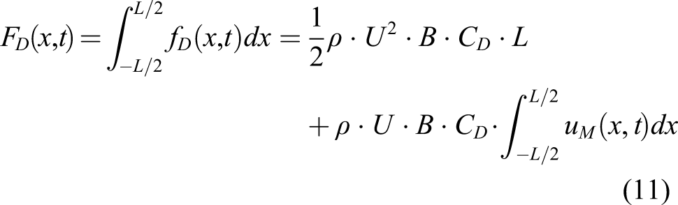
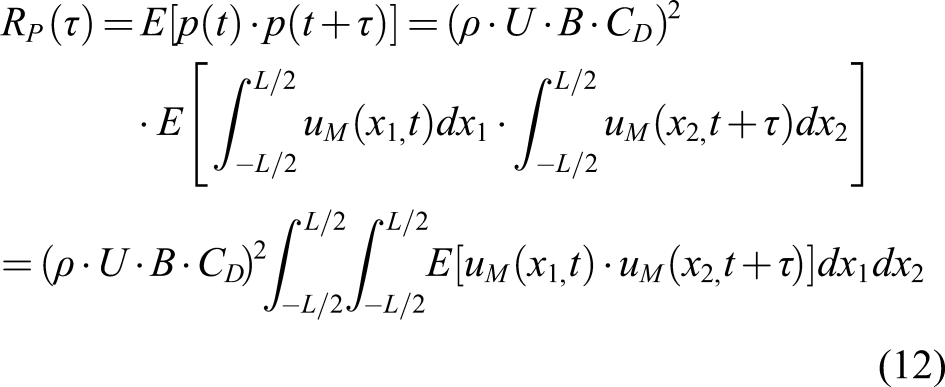
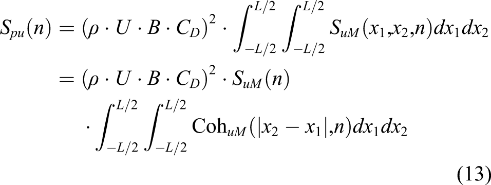

By substituting equation (14) into equation (13), the following equation can be obtained


Similarly, the expression of

As shown in equations (16) and (17), the spanwise correlation functions

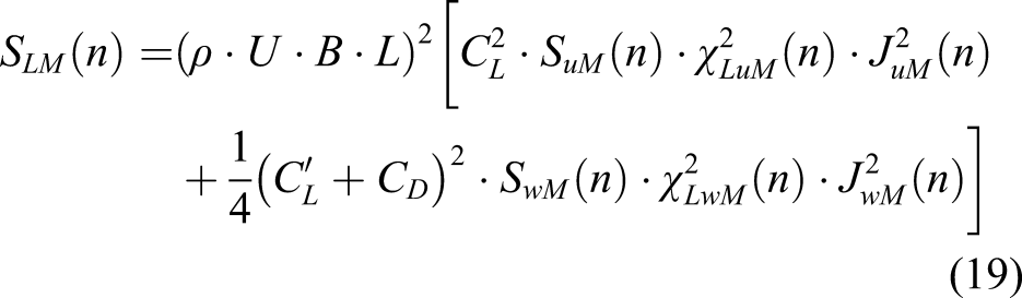
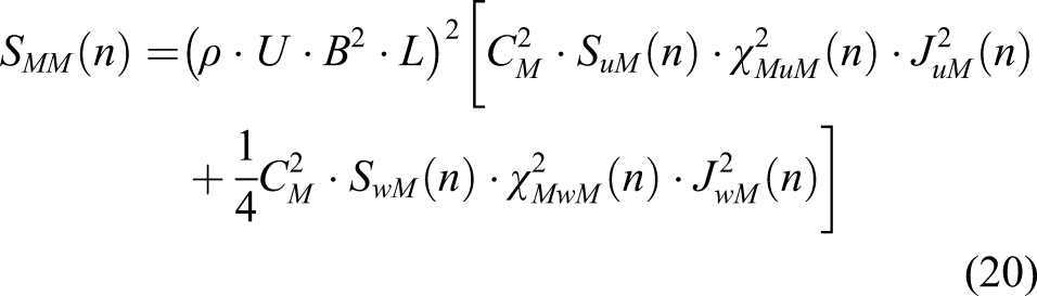
In this paper, a single car was considered to focus on the effects of spanwise correlation of aerodynamic forces on the running vehicle. Then, the time-histories of wind loads on running vehicles can be directly obtained based on equations (18–20). Also, when considering a whole rail vehicle (such as a train) with several cars running along a bridge, the time-histories of buffeting forces acting on each car will be different. Based on the multivariable random process simulation scheme proposed by Shinozuka (1971) or Deodatis (1996), the cross spectral density matrix of buffeting forces acting on different cars can be obtained by the functions of auto-spectra and coherence of the buffeting forces. Then, the time-histories of buffeting forces acting on each car can also be calculated. As for the auto-spectra functions of the buffeting forces, they are given in equations (18–20). However, for the coherence functions of the buffeting forces acting on a running car, there are no quantitative expressions available at present due to the complexity of the running vehicle tests in the wind tunnel (Li et al., 2014). Therefore, the coherence functions of the buffeting forces are usually equal to those of fluctuating wind speeds as an approximation, as given in equations (4) and (8).
Establishment of the rail vehicle-bridge coupling system model
To investigate the effects of spanwise correlation functions in vehicle aerodynamic force on the dynamic responses of the vehicle and bridge, a single CRH3 car running along a typical concrete simply-supported girder bridge was taken as an example, and the rail vehicle-bridge coupling system model should be established first. The commercial software SIMPACK including a wheel-rail module has a high simulation accuracy, which is very suitable to establish the rail vehicle-bridge multibody dynamic model. At present, the commercial software SIMPACK is widely used and approved in the field of rail vehicle. Besides, according to the research by Li et al. (2018) and Xu (2017), the responses of wind-rail vehicle subsystem, wind-bridge subsystem, and rail vehicle-bridge subsystem calculated by SIMPACK were systematically validated by the ANSYS or measurement data, respectively. Therefore, the rail vehicle-bridge system established by the commercial software SIMPACK is credible and effective. For these reasons, the commercial software SIMPACK was adopted in this study, and the modeling method which used in previous studies (Han et al., 2020; Li et al., 2018; Xu, 2017) were also used in the present study.
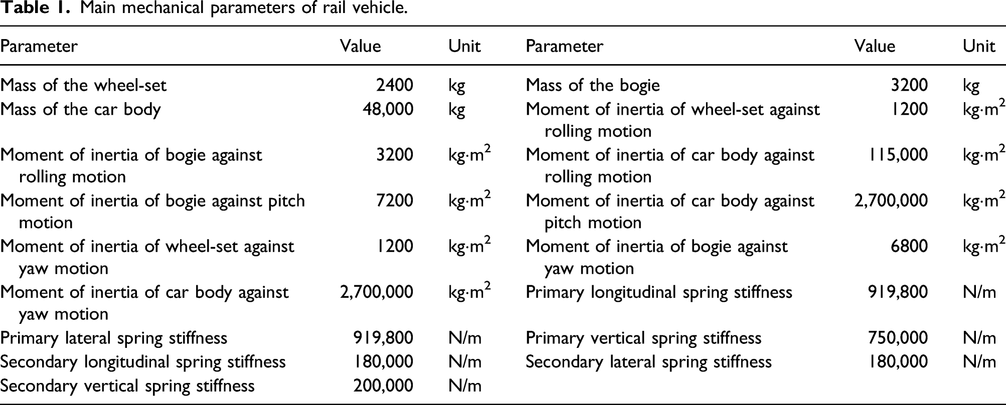
Main mechanical parameters of rail vehicle.
Main mechanical parameters of the bridge and rail.

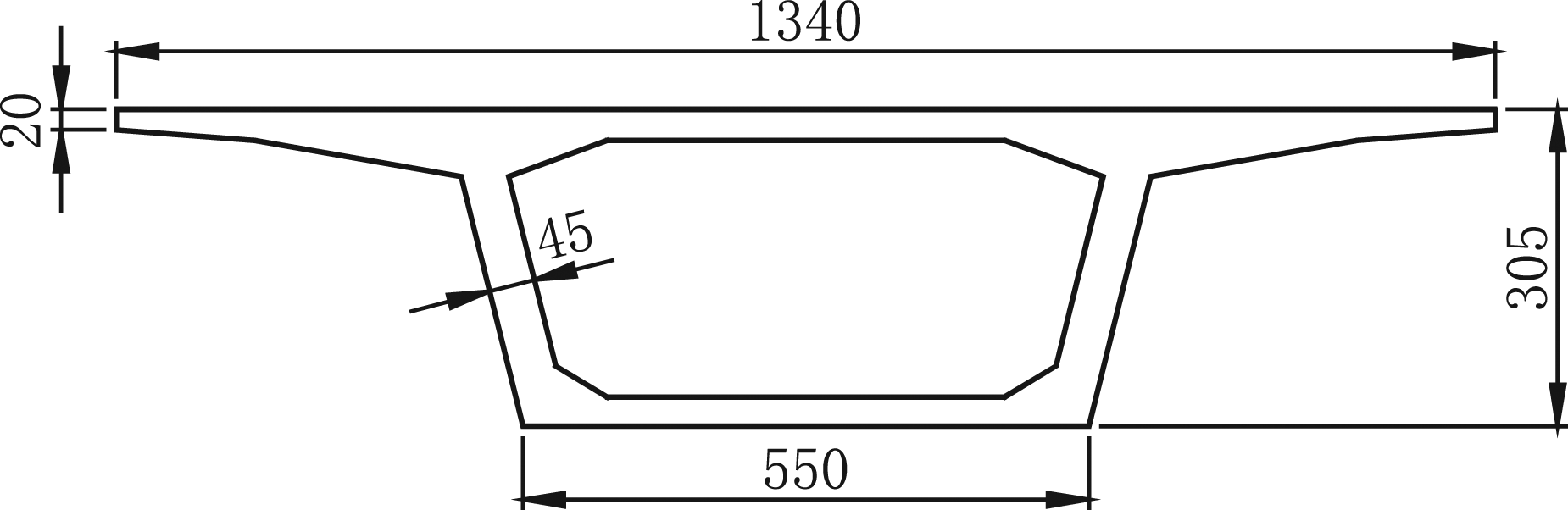
Geometric size of the bridge section (Unit: cm).
In the SIMPACK, when the rail vehicle-bridge multibody dynamic model is established, its residual acceleration value could be obtained. If the residual acceleration value is very small, it means the multibody dynamic model is in equilibrium state and the model is established correctly. Otherwise, the multibody dynamic model is established incorrectly with a large residual acceleration value. Therefore, the residual acceleration value is a parameter to evaluate the accuracy of vehicle-bridge model. Normally, the residual acceleration is generally required to be less than 0.01 m/s2 (Li et al., 2018). By calculating the nominal forces of the rail vehicle-bridge coupling system model established in this study, the residual acceleration of the system is only 1.608 × 10⁻⁷ m/s2, far less than 0.01 m/s2, which thus verifies the accuracy of the model in this study. The final rail vehicle-bridge coupling system model is established as shown in Figure 5, and the first few modes and natural frequencies for vehicle and bridge are listed in Table 3. Simulation model for the rail vehicle-bridge coupling system. First few modes and natural frequencies for vehicle and bridge.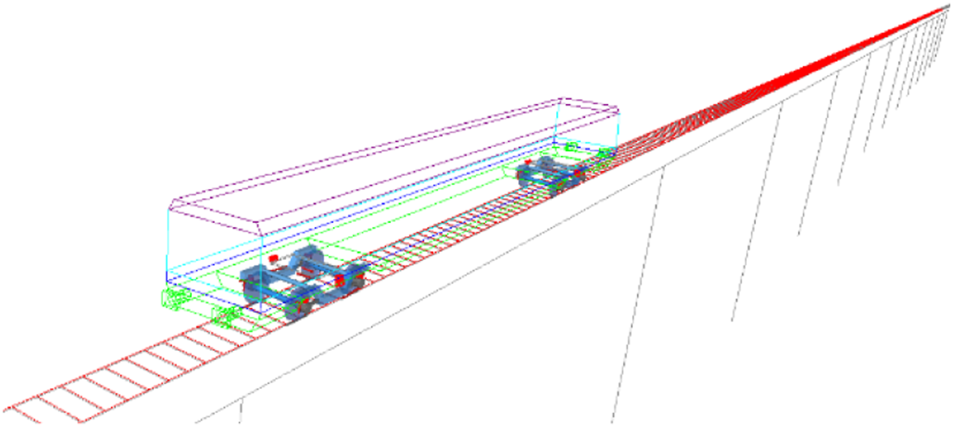

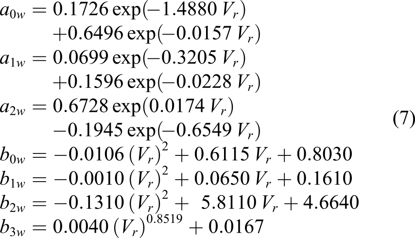
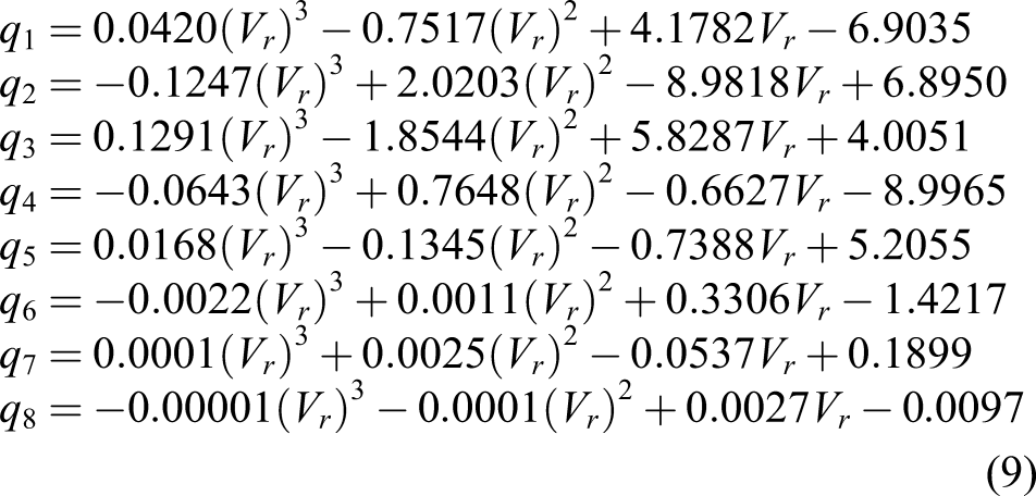
In this study, the height of the center of the vehicle body from the ground is 20.0 m, that is, z = 20.0 m, the mean wind speed U at this height is 25.0 m/s, the surface type belongs to type B terrain (JTG/T 3360-01, 2018), and the vehicle speed V is 60.0 m/s. The spanwise correlation functions in vehicle aerodynamic forces subject to the longitudinal and vertical fluctuating wind speeds can be calculated according to equations (16) and (17) as well as equations (5) and (9), as shown in Figure 6. It can be seen that the higher the frequency, the smaller the values of spanwise correlation functions subject to the longitudinal and vertical fluctuating wind speeds. Spanwise correlation functions 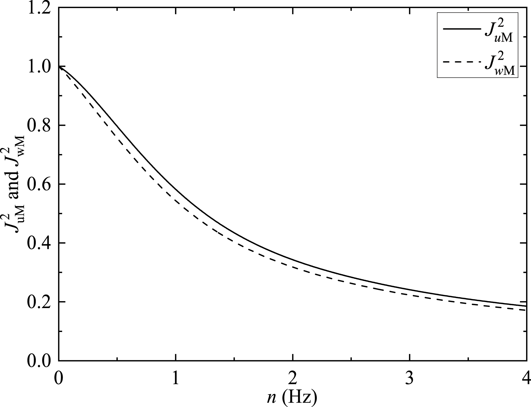



Three-component coefficients of vehicle and bridge.

Effects of spanwise correlation functions on the dynamic responses of the rail vehicle-bridge coupling system
Effects of artificial discrete wind fields on the dynamic responses of the rail vehicle and bridge
The wind loads on vehicles always change with time, which means that it is a continuous function of time. However, the wind loads on vehicles are usually artificially discretized by time in studies on the coupling vibration of wind-rail vehicle-bridge system. This small time discretization will lead to a large space discretization for vehicles running at a high speed. In other words, the high-speed rail vehicle is moving in a “skipping” way on the bridge, which will obviously cause the sudden change in the wind loads on vehicles running at a high speed and the corresponding vehicle dynamic responses will be noticeably affected (Wu et al., 2015). Therefore, it is necessary to first clarify the effects of artificial discrete wind fields on the vehicle dynamic responses when running on the bridge to determine the exact effects of the spanwise correlation function above (equations (16) and (17)).
Since the dynamic responses of rail vehicle and bridge are all stochastic processes, the response results presented in this study are all in the form of root mean square (RMS). Also, the response results of vehicle and bridge under different cases can be directly compared by using the statistical parameter RMS. Taking the vertical acceleration response of the vehicle as an example, Figure 7(a) shows the responses of the running vehicle with different artificial discrete length intervals at a wind speed of 25.0 m/s and vehicle speeds of 40.0 m/s, 60.0 m/s, and 80.0 m/s, respectively, where the discrete length interval is the product of the discrete time interval and the vehicle speed. As shown in the figure, the values of RMS for vehicle vertical acceleration tend to decrease gradually with the increase of discrete length interval at different vehicle speeds. Similarly, Figure 7(b) presents the effects of different artificial discrete length intervals on the vehicle responses when running at a vehicle speed of 60.0 m/s and under wind speeds of 20.0 m/s, 25.0 m/s, and 30.0 m/s, respectively. It can be known that the RMSs of the vehicle vertical acceleration also tend to gradually decrease as the discrete length intervals increase at different wind speeds. Baker (2010) used a discrete time interval of 0.05 s for calculating the time-histories of the wind loads on vehicles, but the reasons for choosing to be 0.05 s were not given clearly. In this study, the corresponding discrete length intervals are 2.0 m, 3.0 m, and 4.0 m at vehicle speeds of 40.0 m/s, 60.0 m/s, and 80.0 m/s, respectively, when the discrete time interval is 0.05 s. If a small discrete length interval of 1.0 m is taken as the reference value, the relative deviation values of vehicle responses at different discrete length intervals relative to those at the reference discrete length interval are listed in Table 5. It is seen that the relative deviation (absolute) values between responses at different vehicle speeds and different wind speeds are all less than 5% if the discrete time interval is determined to be 0.05 s, which gives support to the fact that the response errors caused by the discrete time interval of 0.05 s or the corresponding discrete length interval are relatively small. RMSs of vehicle vertical acceleration changing with the discrete length interval at different vehicle and wind speed. (a) Different vehicle speeds; (b) Different wind speeds. Relative deviation values of vehicle responses at different discrete length intervals relative to those at the reference discrete length interval.

Similarly, the values of RMS for bridge vertical acceleration change with the artificial discrete length interval at different vehicle speeds and wind speeds are shown in Figure 8. Different from the trends presented by Figure 7, no obvious trends could be found in the values of RMS for bridge vertical acceleration with different artificial discrete length intervals. In other words, the RMSs of bridge vertical acceleration are not sensitive to the artificial discrete length interval regarding different vehicle speeds and wind speeds. Comprehensively considering the effects of artificial discrete length interval on the vehicle and bridge responses and to ensure the calculation accuracy of wind loads acting on running vehicles, a discrete time interval of 0.05 s was used for discretizing the wind fields in the subsequent studies. RMSs of bridge vertical acceleration changing with the discrete length interval at different vehicle and wind speeds. (a) Different vehicle speeds; (b) Different wind speeds.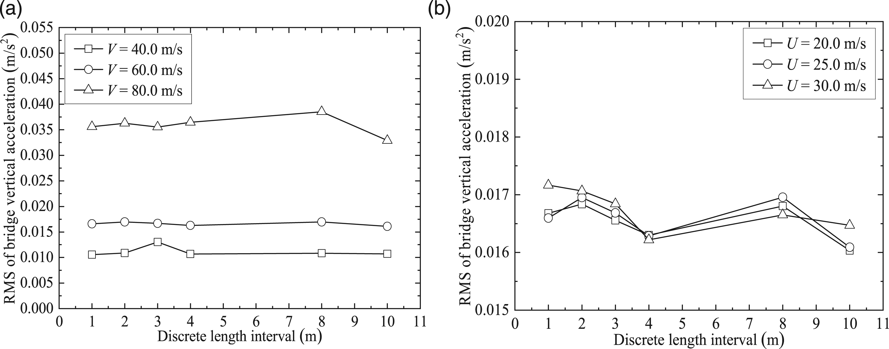
Dynamic responses of the rail vehicle-bridge coupling system at different vehicle speeds
In order to investigate the effects of spanwise correlation functions on the rail vehicle and bridge responses at different vehicle speeds, the analysis was carried out for the rail vehicle-bridge coupling system under five cases with a wind speed of 25.0 m/s and vehicle speeds of 40.0 m/s, 50.0 m/s, 60.0 m/s, 70.0 m/s, and 80.0 m/s, respectively. Each case was analyzed in the presence and absence of the effects of spanwise correlation functions. For vehicle responses, the dynamic results of vehicle lateral acceleration, vehicle vertical acceleration, derailment coefficient, wheel load reduction rate, vehicle lateral Sperling index, vehicle vertical Sperling index, wheel-rail vertical force, and wheel-rail lateral force were investigated. For bridge responses, the dynamic results of bridge vertical acceleration and bridge lateral acceleration were mainly investigated. Taking the lateral acceleration responses of the vehicle and bridge as an example, the time-history results of vehicle and bridge at the wind speed of 25 m/s and vehicle speed of 40 m/s are shown in Figure 9. It is seen that the dynamic results of vehicle and bridge with considering the spanwise correlation functions are generally smaller than those without considering the spanwise correlation functions. Lateral acceleration responses of the vehicle and bridge with/without considering the spanwise correlation functions (“+ SCFs” refers to the case considering the spanwise correlation functions, similarly hereinafter). (a) Vehicle lateral acceleration; (b) Bridge lateral acceleration.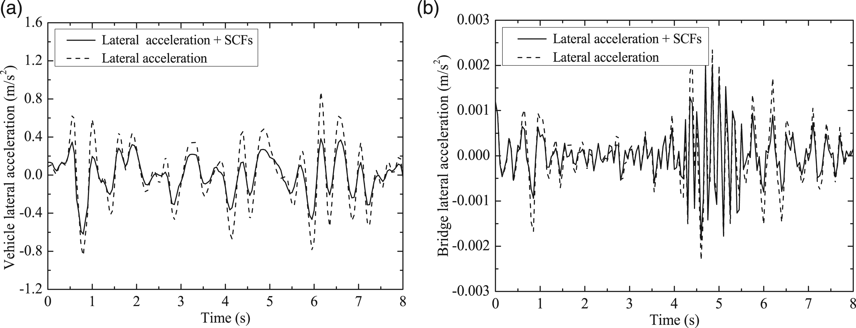
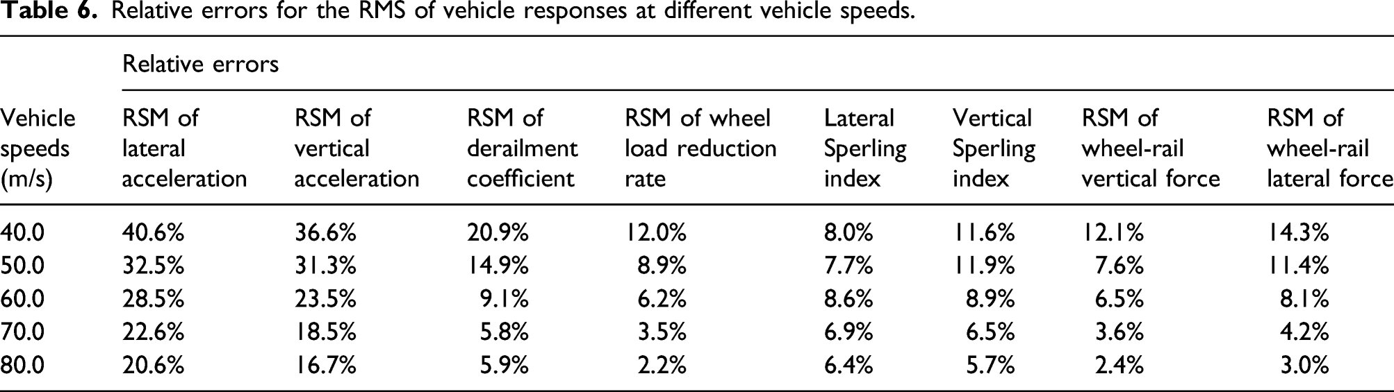
To make comparison of the response results from the aspect of statistics, Figure 10 shows the RMS values of vehicle responses in the presence and absence of spanwise correlation functions at different vehicle speeds. It can be seen that these vehicle responses increase with the increase of vehicle speed regardless of whether the spanwise correlation functions are considered or not. The RMS slopes of wheel-rail force, wheel load reduction rate, and vehicle lateral acceleration are relatively large when the vehicle speed is increased from 40.0 m/s to 80.0 m/s, which supports that higher vehicle speed has more significant effects on these results. Meanwhile, the changes in slope of vehicle vertical and lateral Sperling indexes are small, which indicates that these indexes are insensitive to changes of vehicle speed. In addition, it is noted that with the increase of vehicle speed, the values of vehicle responses in the presence of spanwise correlation functions tend to be close to those in the absence of spanwise correlation functions. This is mainly because the values of coherence function for the fluctuating wind speeds relative to the running vehicle equations (4) and (8) gradually approaches to 1.0 as the velocity ratio Vr (or vehicle speed V) increases. Besides, it can be known from equations (16) and (17) that the values of spanwise correlation functions are also gradually close to 1.0 when the vehicle speed increases. The reflection of these laws in equations (18–20) reveals that with the increase of vehicle speed, the wind loads on the running vehicle show the tendency to be similar in the presence and absence of spanwise correlation functions, which is also the case for the vehicle responses. Vehicle responses at different vehicle speeds. (a) RMS of vehicle acceleration; (b) RMS of derailment factor and wheel load reduction rate; (c) Sperling indexes of vehicle acceleration; (d) RMSs of wheel-rail force.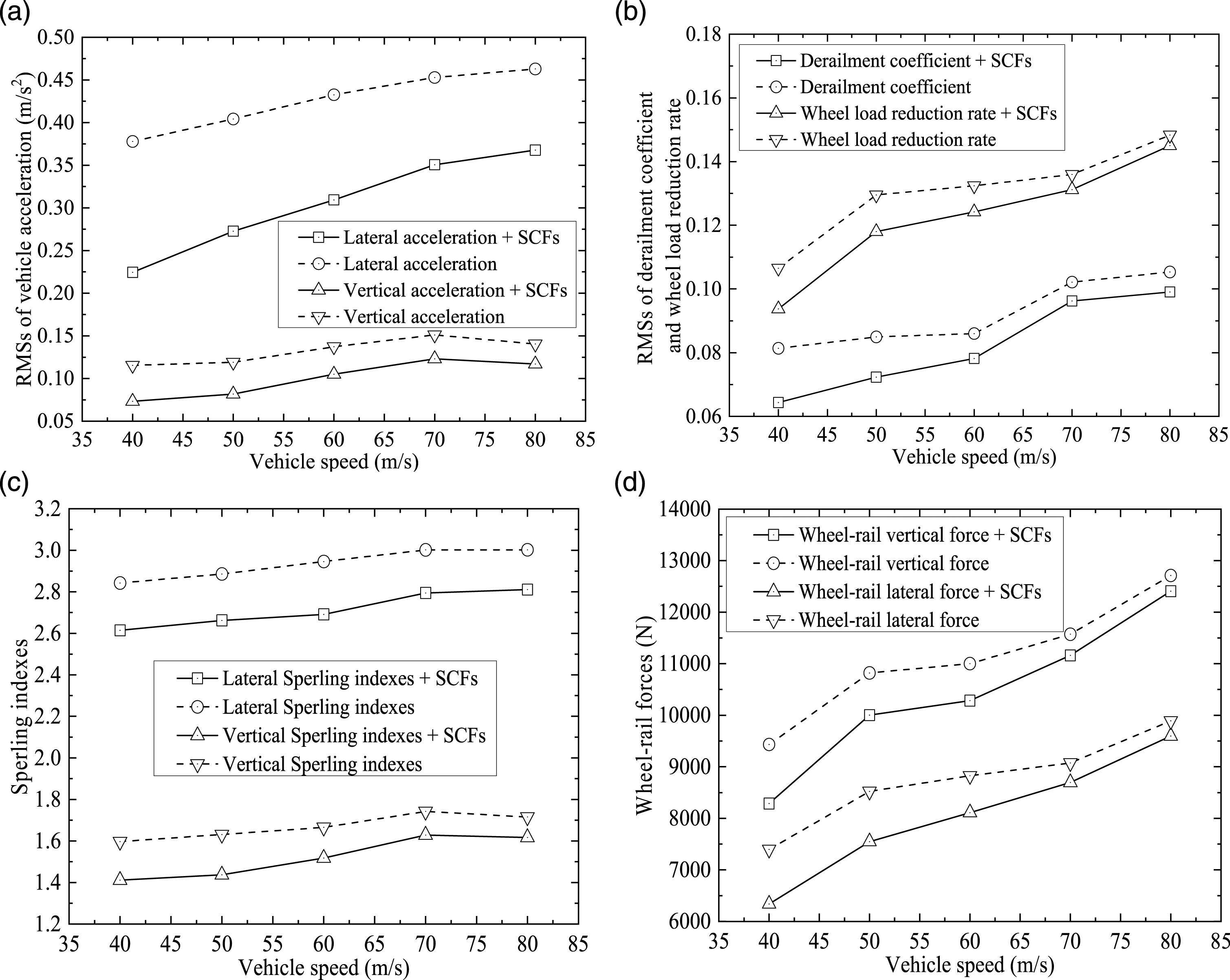
Relative errors for the RMS of vehicle responses at different vehicle speeds.
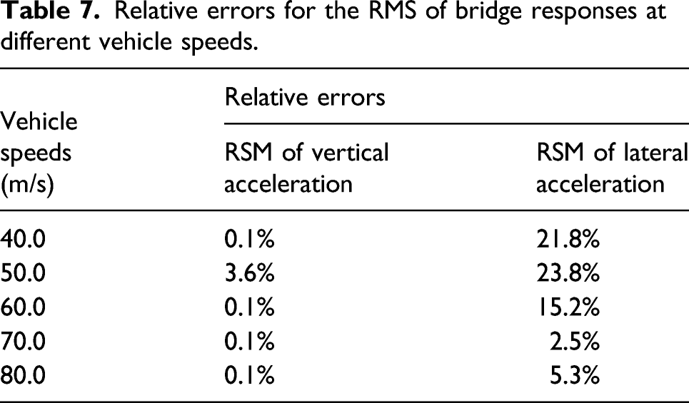
As for the bridge responses, Figure 11 shows the RMSs of vertical and lateral acceleration at the mid-span point of the bridge, it can be seen that the RMSs of the bridge vertical and lateral accelerations increase with the vehicle speeds. When the vehicle speed is increased from 40.0 m/s to 80.0 m/s, the RMS slopes of the bridge vertical acceleration become larger, implying the higher vehicle speed has more significant effects on the RMS of the bridge vertical acceleration. It should be noted that the RMSs of the bridge vertical acceleration with and without considering the spanwise correlation functions are almost the same, indicating that the spanwise correlation functions have little effects on the bridge vertical acceleration. Besides, the RMSs of the bridge lateral acceleration with and without considering the spanwise correlation function are close to each other when the vehicle speed increase, which reflects the spanwise correlation functions have relatively small effects on it at higher vehicle speeds. Obviously, this phenomenon is similar to that presented in Figure 10, which is related to the corresponding vehicle responses and the reasons are not repeated here. Bridge responses at different vehicle speeds. (a) Bridge vertical acceleration; (b) Bridge lateral acceleration.
Relative errors for the RMS of bridge responses at different vehicle speeds.
Dynamic responses of the rail vehicle-bridge coupling system at different wind speeds
In order to investigate the effects of spanwise correlation functions on the vehicle and bridge responses at different wind speeds, the analysis was performed for the rail vehicle-bridge coupling system under five cases with a vehicle speed of 60.0 m/s and wind speeds of 20.0 m/s, 22.5 m/s, 25.0 m/s, 27.5 m/s, and 30.0 m/s, respectively. Figure 12 presents the values of vehicle responses in the presence and absence of spanwise correlation functions at different wind speeds. Vehicle responses at different wind speeds. (a) RMS of vehicle acceleration; (b) RMS of derailment factor and wheel load reduction rate; (c) Sperling indexes of vehicle acceleration; (d) RMSs of wheel-rail force.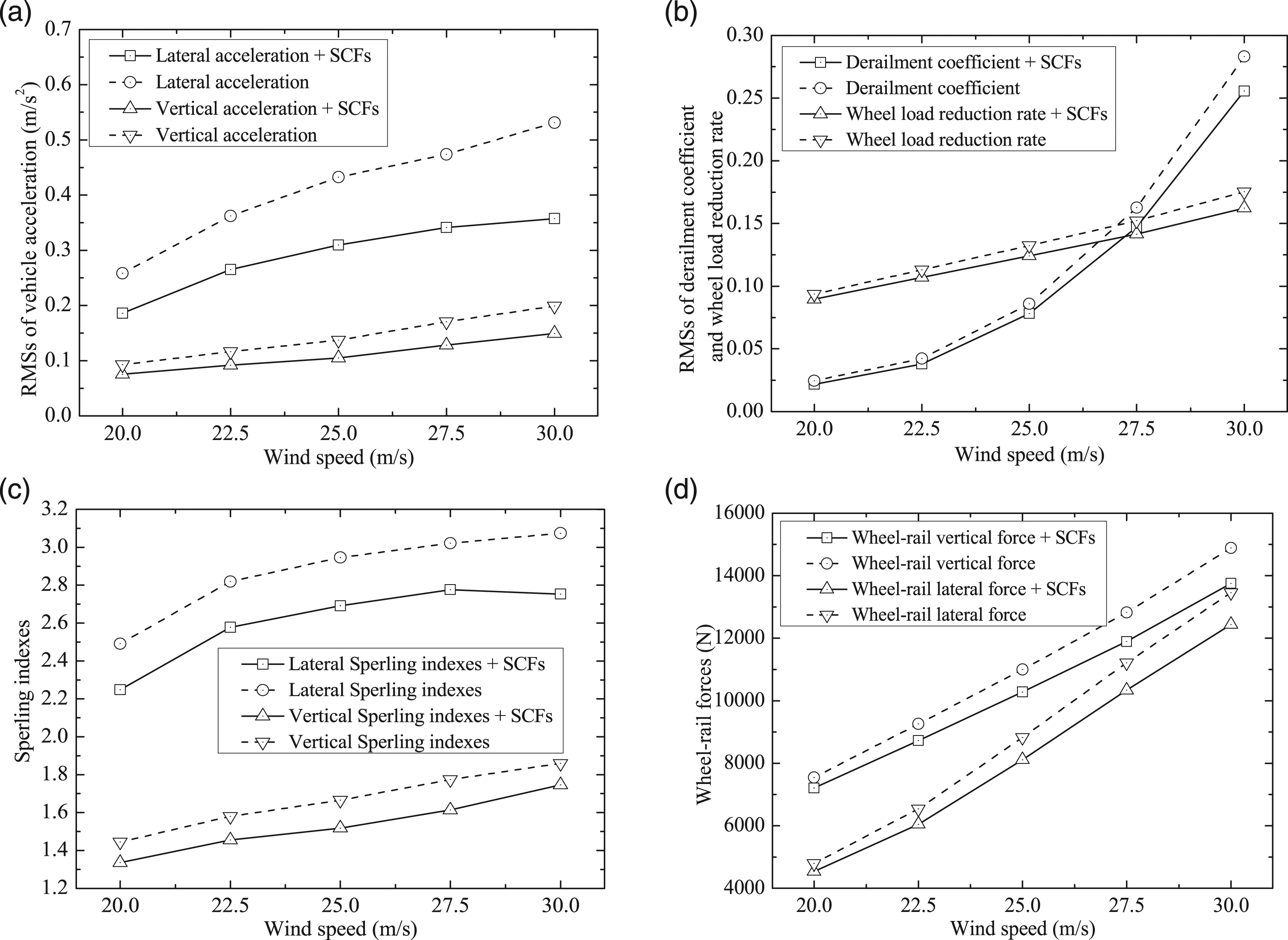
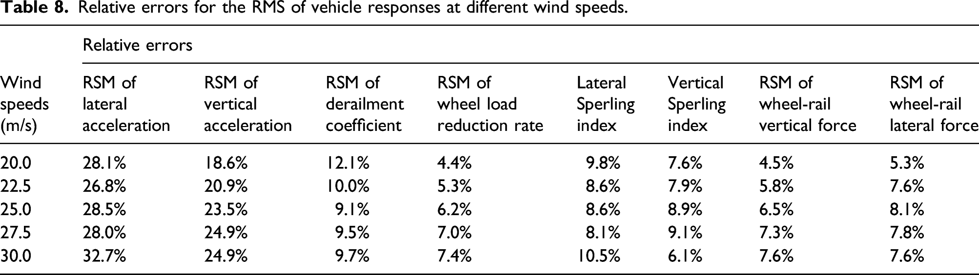
It can be observed that those vehicle responses increase with the increase of wind speed, and the slopes of most vehicle responses are relatively large when the wind speed increases from 20.0 m/s to 30.0 m/s. However, the slopes for the RMSs of vehicle lateral acceleration and vehicle lateral Sperling index have a gradual tendency to flatten, supporting more significant impacts of lower wind speeds on them. Meanwhile, the slopes for the RMS of derailment coefficient become steeper, which proves the significant impacts of higher wind speeds on it. Furthermore, it is noted that as the wind speed increases, the value of each vehicle response generally tends to show a greater difference in the presence and absence of spanwise correlation functions. This is partly because of the decrease in speed ratio Vr and the increase of wind loads when wind speed increases. Due to the combined effects of various factors, the differences between each vehicle response in the presence and absence of spanwise correlation functions are more significant when wind speed increases.
Relative errors for the RMS of vehicle responses at different wind speeds.
Similarly, Figure 13 shows the RMSs of bridge vertical and lateral accelerations at different wind speeds. Obviously, the RMSs of bridge vertical and lateral accelerations increase with the increase of wind speed. For the RMS of bridge vertical acceleration, the spanwise correlation functions have little effects on it. Moreover, the differences of RMSs of bridge lateral acceleration with and without considering the spanwise correlation functions become larger when the wind speed increases, which implies that the spanwise correlation functions have more significant effects on it at higher wind speeds. This phenomenon could also be found in Figure 12, which is associated with the corresponding vehicle responses. Bridge responses at different wind speeds. (a) Bridge vertical acceleration; (b) Bridge lateral acceleration.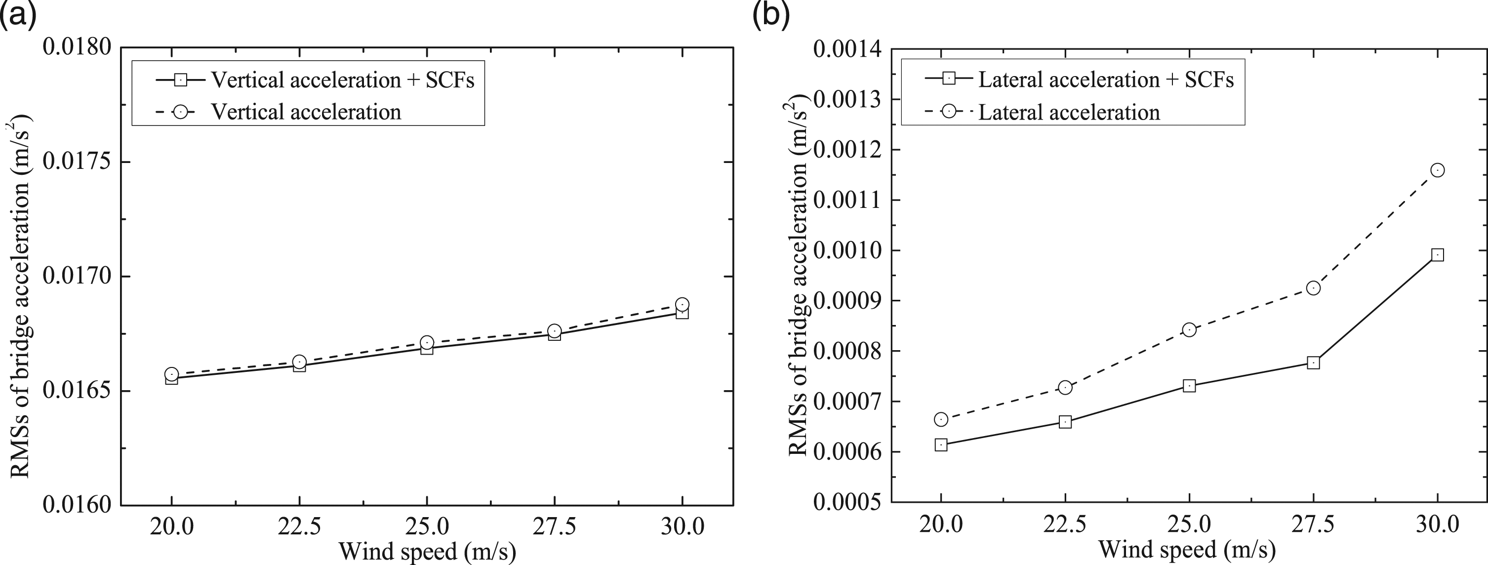
Relative errors for the RMS of bridge responses at different wind speeds.

Conclusion
This paper investigated the effects of spanwise correlation functions in vehicle aerodynamic forces on the dynamic responses of the rail vehicle-bridge coupling system, and the effects of different discrete time intervals, vehicle speeds and wind speeds were analyzed. The main conclusions are as follows: 1. A simplified form of fluctuating wind coherence function relative to the running vehicle were developed, and the spanwise correlation functions in vehicle aerodynamic forces, which corresponds to the longitudinal and vertical fluctuating wind speeds, were proposed. 2. For wind-rail vehicle-bridge system, different discrete time intervals can exert significant effects on the vehicle responses, but they have no obvious effects on the bridge responses. The discrete time interval of 0.05 s could be used for analysis. 3. With the increase of vehicle speed, the values of vehicle and bridge responses in the presence of spanwise correlation functions tend to be close to those in the absence of spanwise correlation functions. However, as the wind speed increases, the values of vehicle and bridge responses generally tend to show greater differences in the presence and absence of spanwise correlation functions. These phenomena are related to the values of spanwise correlation functions changing with the vehicle speed and the wind speed. 4. At different vehicle speeds or wind speeds, the spanwise correlation functions have the most significant effects on the RMSs of vehicle accelerations. When the vehicle speed is 40.0 m/s, the relative errors for the RMSs of vehicle lateral and vertical accelerations are as high as 40.6% and 36.6%, respectively. When the wind speed is 30.0 m/s, the relative errors for the RMSs of vehicle lateral and vertical accelerations are 32.7% and 24.9%, respectively. The relative errors for the RMSs of vehicle responses gradually decrease as the vehicle speed increases. With the wind speed increasing, the relative errors for the RMS of wheel load reduction rate and wheel-rail vertical force gradually increase, but the relative errors for the vehicle vertical Sperling index and the RMS of wheel-rail lateral force first increase then decrease. 5. At different vehicle speeds or wind speeds, the spanwise correlation functions have significant effects on the bridge lateral acceleration, but they have little effects on the bridge vertical acceleration. With the increase of the vehicle speed, the relative errors for the RMSs of bridge lateral acceleration generally decrease. However, the relative errors for the RMSs of bridge lateral acceleration generally increase with the increase of the wind speed. Particularly, when the vehicle speed is 50.0 m/s, the relative error for the RMS of the bridge lateral acceleration reaches up to 23.8%, and it is about 17.0% when the wind speed is 30.0 m/s.
Footnotes
Declaration of conflicting interests
The author(s) declared no potential conflicts of interest with respect to the research, authorship, and/or publication of this article.
Funding
The author(s) disclosed receipt of the following financial support for the research, authorship, and/or publication of this article: This work was supported by National Natural Science Foundation of China under grant Nos. 51878080, 52178451 and 51822803, the Hunan Provincial Natural Science Foundation of China under grant Nos. 2020JJ3035 and 2018JJ3538, and “Double First-Class” scientific research international cooperation and development project of Changsha University of Science & Technology under grant No 2019IC01.
