Buckling critical load prediction of pultruded fiber-reinforced polymer columns and feature analysis by machine learning

Abstract

For slender FRP columns, predicting the global buckling critical loads is crucial in structural design. However, there is a lack of a consensus prediction method based on specialized domain knowledge. To address this issue, this study created a comprehensive database by collecting 365 experimental data related to global buckling of axially loaded pultruded FRP columns to predict buckling critical loads using such machine learning methods as extreme gradient boosting, artificial neural network, and support vector regression. The prediction accuracy and stability of the machine learning prediction methods were evaluated, and the interpretability of the features was analyzed in depth. The results show that the prediction accuracy of the traditional theoretical methods is low, while that of the machine learning methods is high. The contribution of geometric parameters to the buckling critical load is more than 80%. The contribution of material parameters to the buckling critical load is small, less than 20%. The cross-sectional moment of inertia has the most significant effect on the buckling critical load, while the shear modulus and compressive strength have a smaller effect.

Keywords

buckling critical load extreme gradient boosting artificial neural network support vector regression machine learning pultruded fiber-reinforced polymer feature analysis

Introduction

Compared to traditional steel and reinforced concrete pressure-bearing columns, fiber-reinforced polymer (FRP) composites have high strength and low modulus, which increases their vulnerability to global flexural buckling failure (Zhan et al., 2018; Zhan and Wu, 2018a). Moreover, when FRP members undergo global flexural buckling, they exhibit poor ductility due to their linear elastic mechanical properties without a yield stage or plastic deformation (Boscato et al., 2014). The mechanical properties and mechanical response of pultruded FRP members are complex, which contributes to the uncertainty of bending buckling (Higgoda et al., 2023a). Additionally, the susceptibility of FRP columns to flexural buckling is affected by the non-uniform distribution of fiber resin across their cross-section (Feng et al., 2022). The difference in mechanical properties between FRP composites and traditional materials leads to a significant difference in predicting the critical load of global flexural buckling of pultruded FRP struts from isotropic materials (Jerath, 2021). Therefore, predicting critical loads for global flexural buckling of FRP columns becomes a significant and complex problem (Sá et al., 2021; Pacheco et al., 2021).

For PFRP struts of sufficient slenderness that fail by global buckling, (Barbero and Tomblin, 1993; Barbero and Raftoyiannis, 1993; Seangatith and Sriboonlue, 1999; Hashem and Yuan, 2001; Hewson, 1978) have demonstrated through experimental, numerical, and analytical work that the critical global buckling load can be predicted with reasonable accuracy using the classical Euler formula given by equation (1).

P_{E} = π E I / L^{2}

(1)

where

P_{E}

is the Euler critical load.

E

is elastic modulus;

I

denotes weak axis moment of inertia of section;

L

denotes effective length. However, there has yet to be a consensus on applying the classical Euler formula based on isotropic materials to anisotropic FRP struts. Some scholars suggest using the Euler formula to predict the buckling critical load of pultruded FRP compression columns by replacing the elastic modulus in equation (1) with the axial compression modulus of the FRP column (Seangatith and Sriboonlue, 1999; Hashem and Yuan, 2001; Goodman and Gliksman, 1969). Others believe that the flexural modulus of the FRP column should be used to replace the modulus of elasticity in equation (1) (Hewson, 1978). Still, others do not recommend replacing the modulus of elasticity in equation (1) alone but rather replacing the flexural stiffness (EI) as a whole (Barbero and Tomblin, 1993; Barbero and Raftoyiannis, 1993; Iyengar, 1988; Li et al., 2020).

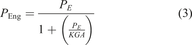
Pultruded FRP members have a notable characteristic of higher longitudinal elastic modulus to in-plane shear modulus ratio. Shear deformation can have a negative impact on the global flexural buckling of these members. Therefore, when predicting the critical load for buckling, it is crucial to consider the effect of shear deformation. Two well-known theories of shear deformation, Haringx and Engesser theories, have been developed to predict critical load, but their applicability and accuracy are subject to great controversy. According to certain scholars, Haringx’s shear modification formula (equation (2)) is a more precise method for predicting the buckling critical load of pultruded FRP members (Kardomateas and Dancila, 1997; Cardoso et al., 2014). However, other scholars argue that Engesser’s shear correction formula (equation (3)) is a more reliable approach for making such predictions (Lee and Hewson, 1979; Roberts, 2002; Bank LC, 2006; Vanevenhoven et al., 2010; Boscato et al., 2015).

P_{Har} = [\sqrt{1 + (\frac{4 P_{E}}{K G A})} - 1] \frac{K G A}{2}

(2)

P_{Eng} = \frac{P_{E}}{1 + (\frac{P_{E}}{K G A})}

(3)

where

P_{Eng}

and

P_{Har}

represent the critical loads calculated from Engesser’s and Haringx’s theories, respectively.

K G A

denotes the shear stiffness of the cross-section,

G

represents the in-plane shear modulus, and

K

represents the shear coefficient of the cross-section.

In addition to the above-mentioned critical load prediction method based on the buckling criterion, there is also an empirical formula represented by the Ayrton-Perry formula (equation. (4)), which is based on the regression of experimental data and is used to predict the global buckling critical load of imperfect columns.

P_{A P F} = \frac{f A}{2 λ_{n}^{2}} [(1 + ε_{0} + λ_{n}^{2}) - \sqrt{{(1 + ε_{0} + λ_{n}^{2})}^{2} - 4 λ_{n}^{2}}]

(4)

where

ε_{0}

is the relative initial bending rate.

λ_{n}

is the regularized slenderness ratio.

A

denotes cross-sectional area. For isotropic materials, f denotes the yield strength. For pultruded FRP materials,

f

denotes different strength values depending on the FRP member. When the FRP column is a thick-walled or solid member, the failure mode of the column changes from global buckling to axial compression failure with the decrease of slenderness ratio. The axial compression strength can be regarded as the critical buckling stress limit;

f

denotes the axial compression strength

f_{LC}

. For thin-walled members, as the slenderness ratio decreases, the failure mode of the member may change from global bending buckling to local buckling. The local buckling strength can be regarded as the critical buckling stress limit, and then f denotes the local buckling strength.

However, this method requires fitting the relative initial bending rate. The polynomial equations used for fitting have always been uncertain and freely chosen by different scholars. For example, (Wang et al., 2016; Liu, 2020) chose the form of a simple linear polynomial $ε_{0} = a + b λ_{n}$ to fit. (Zhan et al., 2018; Zhan and Wu, 2018a; Zhan and Wu, 2018b; Feng et al., 2008) chose the quadratic polynomial $ε_{0} = a + b λ_{n}^{2}$ according to the relevant technical regulations of cold-formed thin-walled steel structure, while (Zhang et al., 2014; Zhang, 2019) chose the quadratic trinomial. (Hou et al., 2010; Li, 2019) believed that the variation of the relative initial bending of pultruded FRP members with the regularized slenderness ratio is close to the cubic polynomial function curve, so the cubic polynomial is selected to fit. (Ding et al., 2018) chose the fourth-order polynomial to fit the relative initial bending when predicting the critical bending capacity of basalt-pultruded FRP circular tube members. Therefore, there is no fixed form of the polynomial equation to fit in the regression fitting of the Ayrton-Perry formula.

In summary, the global buckling of FRP columns is a very important area of research. Although several methods have been proposed for calculating the critical load for the global buckling of FRP columns, specific criteria have yet to be recognized. Thus, it is challenging to accurately predict the critical load for the global buckling of FRP columns due to their low modulus, anisotropy, and inhomogeneous resin distribution. In this case, the derivations of empirical or closed-form solutions using experiments or physics-based models are time-consuming and complex. Therefore, using machine learning-based models is an alternative approach to overcome the limitations of physics-based models (Thai, 2022).

In 1996, (Mukherjee et al., 1996) made the first attempt to model the nonlinear behavior of columns (mild steel bars) to predict a buckling load using an artificial neural network (ANN). (Sheidaii and Bahraminejad, 2012) also examined the global buckling of columns, but they focused on the post-buckling behavior and equilibrium paths. They used an ANN to predict the load-displacement curves of columns and developed the relationship between the critical load and member slenderness. At the same time, (Nguyen et al., 2021) developed an effective ANN for predicting the critical buckling load of the WTIS columns. (Kumar and Yadav, 2013) used an ANN approach to calculate the global buckling load of a beam-column with different end conditions. (Xu et al., 2021) used machine-learning algorithms to establish a unified method for the capacity prediction of stainless-steel columns that accounts for different failure modes, materials, and mechanical properties.

The above research results show that machine learning methods provide the excellent accuracy in predicting global buckling critical load. Machine learning technology has significant advantages in dealing with prediction under complex parameters and can be used as a potential solution. Compared with rule-based predictive analysis, machine learning algorithms are more efficient and powerful in automatically extracting useful patterns from large-scale high-dimensional data without relying on data engineering and domain knowledge.

In the above studies, ANN has become the mainstream machine learning algorithm for buckling strength prediction due to its ease of use and high interpretability. In contrast, other machine learning algorithms, such as Support Vector Regression (SVR) and eXtreme Gradient Boosting (XGBoost) (Xu et al., 2021), are rarely used. In addition, previous studies have focused on predicting the overall buckling performance of isotropic material columns. The prediction of the overall buckling critical load of anisotropic material columns has yet to be reported. However, the machine learning research method for isotropic columns provides a reliable theoretical and technical basis for predicting the buckling critical load of pultruded FRP columns.

The previous discussion shows that there is still a need to develop tools to predict the global buckling critical load of pultruded struts. In this study, three machine learning methods were used to predict the buckling critical load of pultruded FRP columns. Therefore, experimental data of pultruded FRP columns were collected to establish an experimental database. Secondly, three typical machine learning models commonly used for regression prediction were established to predict the flexural buckling critical load of pultruded FRP columns, including SVR, ANN, and XGBoost. The prediction accuracy and stability of the three machine learning models are also evaluated. Finally, based on the SHAP value method, the importance of input features is analyzed to explore the influence of input features on the critical load of flexural buckling of pultruded FRP columns. The term “column” used in this paper only refers to axially stressed members.

Establishment and analysis of the experimental database

Establishment of the experimental database

The experimental database is developed for machine learning models to predict the global buckling critical load of FRP columns. The data in the database were obtained from published literature. The suitability of the results for the experimental database was assessed using carefully established selection criteria to ensure the experimental data’s consistency and reliability. A final database of 365 specimens was formed after rigorous screening. The selection rules were as follows: (1) The specimens were fabricated by the pultrusion process using a single, identified fiber and resin type. (2) Geometric parameters, including the cross-sectional moment of inertia

I

, the cross-sectional area

A

, and effective length

L

. (3) Material parameters, including longitudinal compressive elastic modulus

E_{LC}

, in-plane shear modulus

G_{LT}

, and compression strength

f_{LC}

(4) Specimens exhibited a global flexural buckling failure for which the experimentally obtained critical buckling load

P_{\exp}

was reported. Specimens that only provided the buckling capacity derived from Southwell’s method were excluded due to anticipated errors. The complete experimental database assembled in the present study is provided in Table 1.

Table 1.

The Experimental Database for Flexure Buckling of Axially Loaded Pultruded FRP Columns.

Cross section	Quantity	Specimen geometry			Material parameters			P_exp (kN)	Reference
Cross section	Quantity	L (mm)	I (mm⁴)	A (mm²)	E_LC (GPa)	G_LT (GPa)	f_LC (MPa)	P_exp (kN)	Reference
C-section	4	226∼233	610∼1491	86∼100	53.5	8.8	231	5∼11	(Cardoso et al., 2014)
WF-section	16	2980∼6030	1111847∼5631691	1854.84∼4175	23.9∼24.3	3.3∼3.4	263∼268	12∼79	(Hewson, 1978)
NF-section	11	1319∼2532	1133904∼5569965	1876∼4152	17.4∼21.6	4.1∼4.8	304∼331	33∼494	(Barbero and Tomblin, 1993)
Square tube	11	1313∼2543	1450685∼3744591	1782∼2447	25.2∼28.3	3.9∼5.7	320∼396	54∼334	(Barbero and Tomblin, 1993)
WF-section	36	1214∼4874	1111847∼34724974	1855∼9354	22.5	3.2	219	21∼733	(Zureick and Scott, 1997)
NF-section	15	906∼3616	140641∼1678187	1210∼3690	22.5	3.2	219	13∼427	(Zureick and Scott, 1997)
Square tube	15	609∼4862	240634∼3674543	968∼1419	22.5	3.2	219	13∼357	(Zureick and Scott, 1997)
L-section	5	965∼1575	209960∼738221	927∼1845	19.9∼21.4	3.9∼4.5	337∼365	12∼52	(Seangatith and Sriboonlue, 1999)
Square tube	6	2630∼3850	11,736,400	4666	26.7	2.5	149	185∼460	(Zureick and Steffen, 2000)
NF-section	11	3100∼3800	13,332,666	5625	24.3∼24.6	3.4∼3.4	267∼271	215∼322	(Hashem and Yuan, 2001)
NF-section	20	3300∼6300	5740000∼17800000	4210∼7530	23.2	3.5	291	28∼354	(Lane and Mottram, 2002)
NF-section	18	360∼2500	292,437	1792	23.2	5.8	400	11∼463	(Mottram et al., 2003)
WF-section	6	2500∼2800	20,014,167	7700	23.2	5.8	400	478∼607	(Mottram et al., 2003)
Round tube	26	1330∼4000	62580∼138976	270∼511	28∼32	3.9∼4.5	305∼354	0.9∼16	(Blandford, 2010)
Square tube	46	1372∼2073	2,395,499	2097	25.2∼29.0	2.7	189∼243	95∼377	(Puente et al., 2006)
Round tube	4	1632∼2331	1,964,991	1772	44	6.3	340	136∼347	(Blandford, 2010)
L-section	10	316∼2940	18797∼2235184	304∼3715	46	6.4	482	61∼395	(Wang et al., 2011)
Round tube	9	1268∼2331	961063∼16020414	1395∼4323	45.1	2.5	369	136∼1082	(Zhang et al., 2011)
NF-section	1	1540	217,944	1368	28.9	3.9	360	25	(Xu et al., 2013)
Square tube	39	226∼2141	23825∼3697923	284∼2437	22.1∼31.1	2.1∼2.7	224∼333	12∼416	(Nunes et al., 2013)
Round tube	15	420∼2580	25385∼871792	232∼1880	46	6.4	482	9∼410	(Zhang et al., 2014)
NF-section	5	2046	1,681,667	3800	35.3∼41.2	4.9∼5.8	388∼453	133∼155	(Nunes et al., 2016)
Round tube	4	350∼450	8432	138	105	4.6	400	32∼49	(Sun, 2018)
Square tube	1	3080	5,065,408	3515	32.2	3.5	290	155.9	(Xie et al., 2019)
Round tube	6	320∼520	8432	138	33.15	4.1	317	9∼23	(Liu, 2020)
Round tube	3	1210	375,596	1018	63	13	406	134∼141	(Li et al., 2021)
L-section	12	1029∼1336	60,855	612	31.2	2.7	498	8∼16	(Monteiro and Malite, 2021)
Round tube	3	922∼1569	413,383	804	41.5	3.2	617	61∼140	(Feng et al., 2021)
C-section	5	350∼980	56686∼78740	780∼942	34.3	5.5	552	22.8∼133	(Wu et al., 2022)
Round tube	2	1368∼1710	3,142,030	2163	33.3	4.3	485	277∼434	(Higgoda et al., 2023b)
Summary	365	226∼6300	610∼34724973	86∼9355	17.4∼105	2.1∼13	148∼617	0.9∼1081

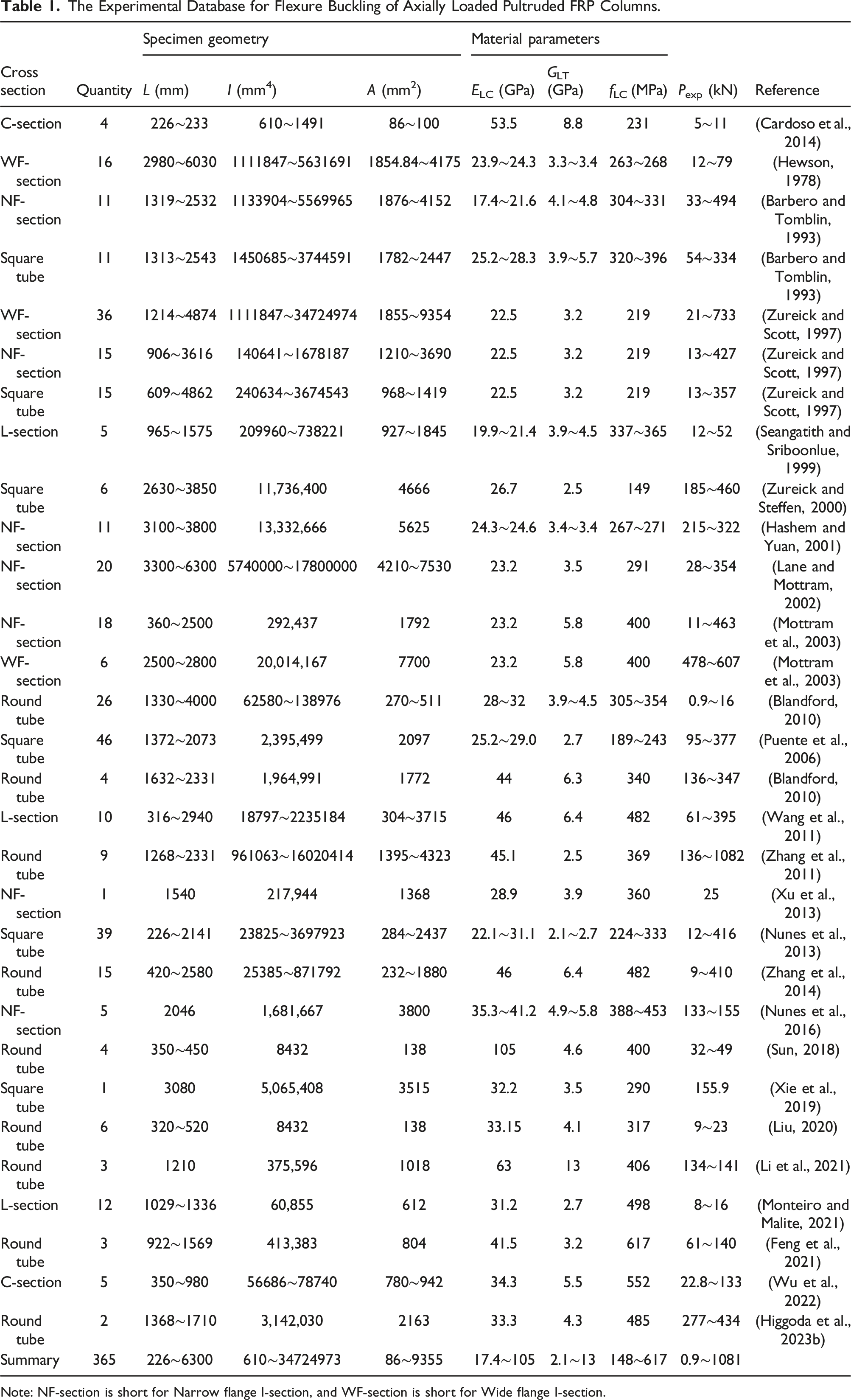
Note: NF-section is short for Narrow flange I-section, and WF-section is short for Wide flange I-section.

Analysis of the experimental database

Previous studies of axial behavior of pultruded FRP have identified the following general conclusions as summarized by (Zureick and Scott, 1997): (a) short columns, $λ_{n} < \approx 0.7$ ; (b) slender columns, $λ_{n} > \approx 1.3$ ; and (c) so-called intermediate columns, having slenderness falling between short and slender columns. The regularized slenderness ratios of the 365 groups of experimental specimens collected in this paper ranged from 0.79 to 8.77, of which 312 groups belonged to slender columns, 53 columns of intermediate columns, and no short columns, as shown in Figure 1. This is because one of the criteria for selecting data collection was the requirement of overall flexural buckling damage of the FRP specimens, while short columns usually do not experience overall flexural buckling. The database covers both intermediate and slender columns. Hence, the machine learning model built from this database is applicable to both intermediate and slender FRP columns.

Figure 1.

Specimen regularized slenderness ratio distribution statistics.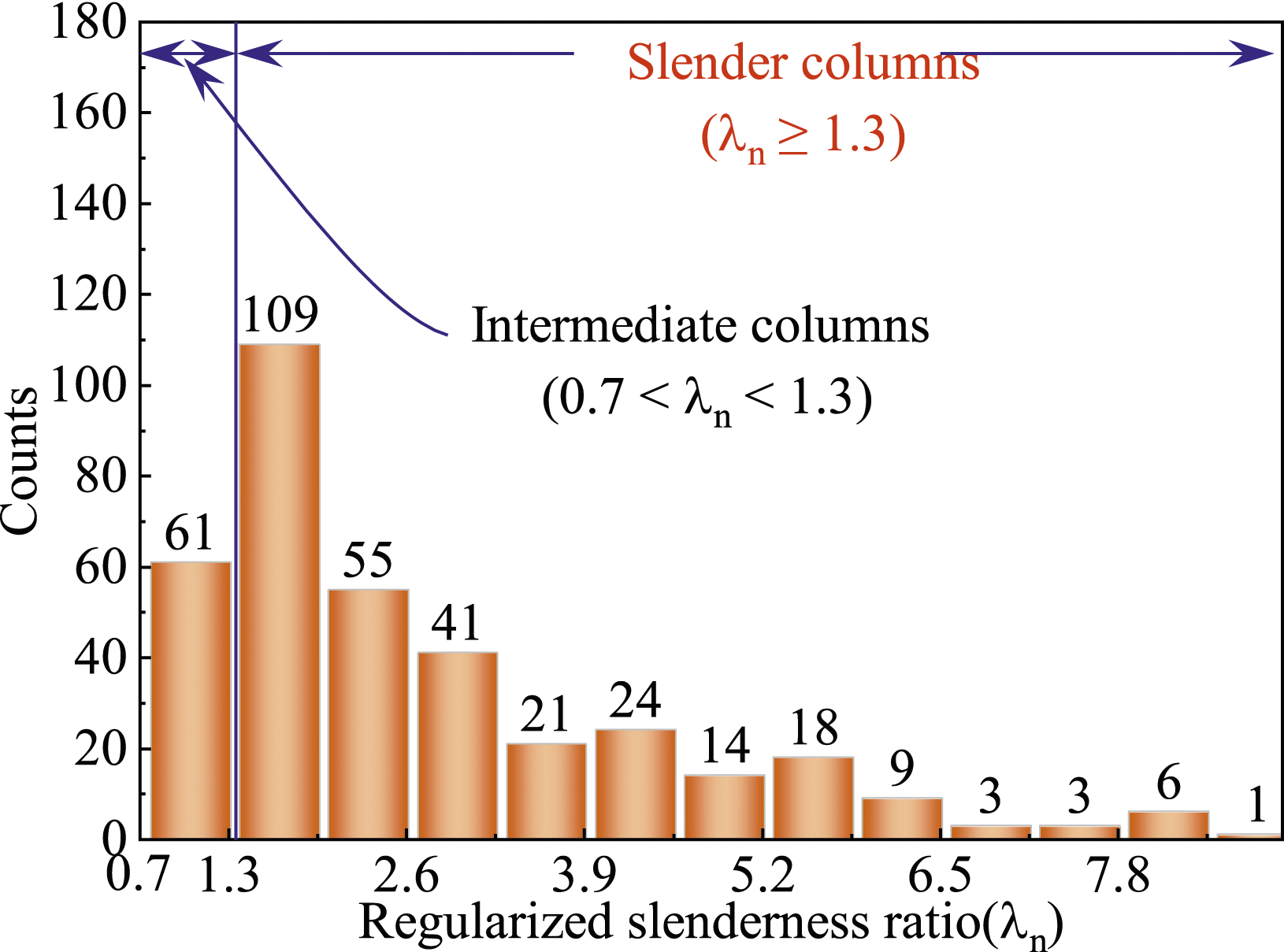

The distribution of the section types of the 365 groups of experimental specimens is shown in Figure 2. Figure 2 shows that the number of square tubes is the largest, followed by round tubes and the least number of slotted cross-sections. The number of specimens with square and round tubes together accounted for 52% of the total number of specimens. The number of specimens with other cross-sections accounted for 48% of the total number of specimens, that is, there were a comparable number of FRP columns in the form of closed cross-sections as those in the form of open cross-sections.

Figure 2.

Distribution of cross-section types.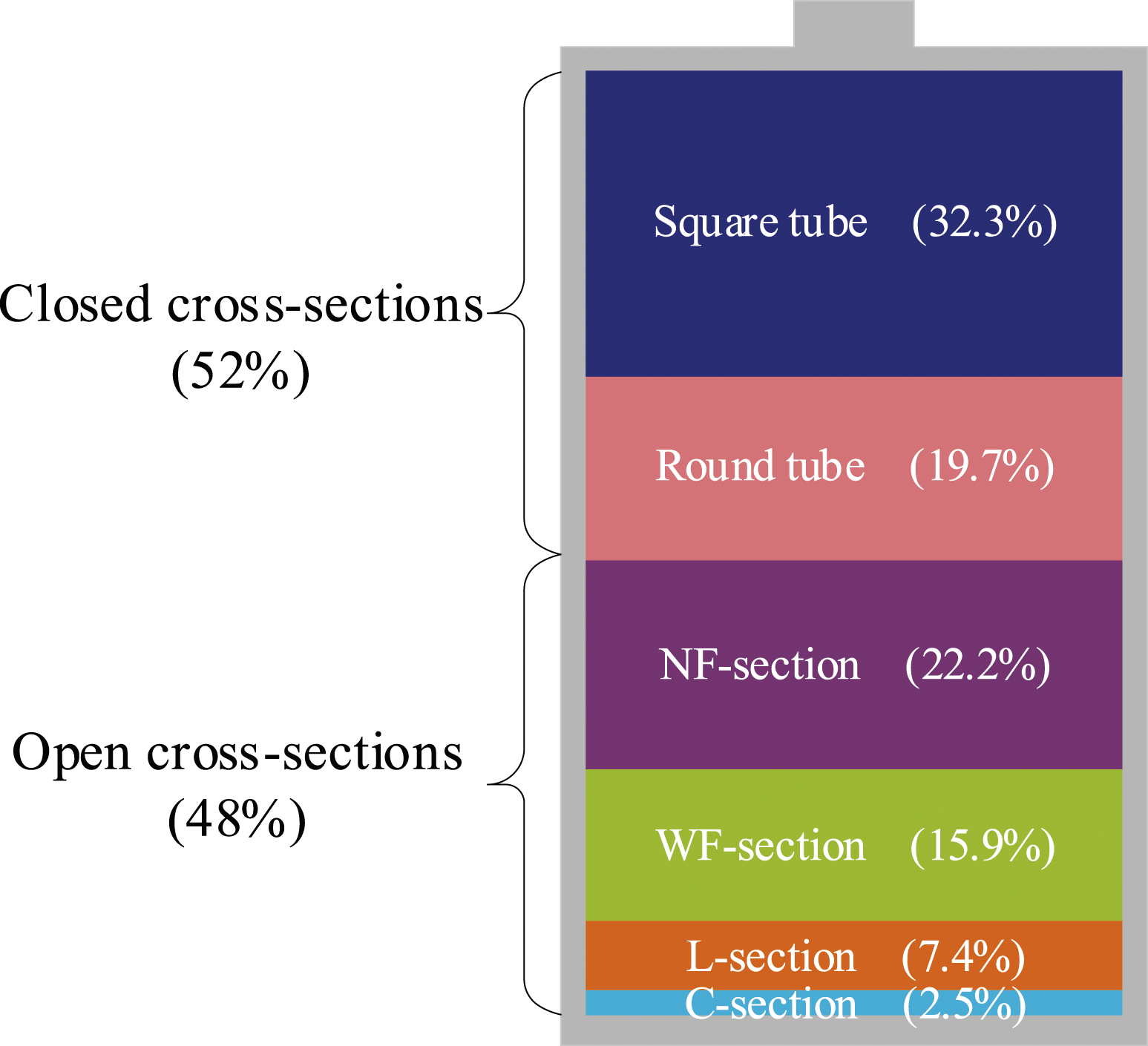

Therefore, the machine learning model trained with this database is applicable not only to FRP columns with closed cross-sections but also to FRP columns with open cross-sections.

Machine learning model

This section will follow the general workflow of machine learning in regression prediction (see Figure 3) for modeling. In addition to the collection and organization of raw data already done in the previous section, the following tasks are included: data preprocessing, machine learning algorithms, hyperparameter optimization, and performance evaluation metrics. The algorithms involved in building machine learning models in this paper are XGBoost, SVR, and ANN. The preparatory knowledge and basic principles of these machine learning algorithms can be found elsewhere, so they will be avoided.

Figure 3.

Typical workflow of Machine Learning.

Data pre-processing

The accuracy of machine learning model predictions depends greatly on the merit of the initial dataset. Therefore, before building the machine learning model, analyze the features to remove redundant data. The initial dataset is normalized or standardized to improve the learning efficiency and the generalization ability of the machine learning model.

The effective length, cross-sectional area, moment of inertia, compressive modulus, shear modulus, and compressive strength are input variables, while the buckling critical load is used as the target variable. The Pearson correlation analysis of the features was carried out, and the results are shown in Figure 4. Positive values indicate a positive correlation, while negative values represent a negative correlation. Except for the moment of inertia, almost all input features have low correlation coefficients with the output feature, remaining between −0.068 and −0.13. There is no strong linear correlation between the input features, indicating that all input features are necessary.

Figure 4.

Pearson correlation of features.

Figure 5 shows the distribution histogram of the six input parameters and one output parameter in this study.

Figure 5.

Statistical distributions of both input and output parameters.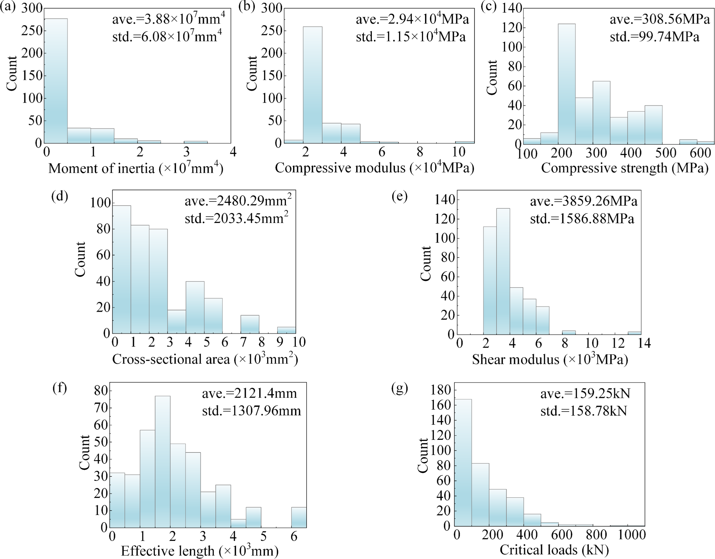

It can be seen that: (1) most of the test specimens have smaller cross-sectional moments of inertia and compression moduli. Therefore, the critical loads of most of the test specimens are also small. (2) The compressive strength of the material parameters of the test data were significantly different. (3) The number of test specimens decreased as the critical load of the members increased, and the critical load of the members for a few test data exceeds 6000.

Simultaneously, considering that the difference between the mean values of the input features (Table 1) is significant, to avoid poor model calculation results, it is essential to standardize the data. Figure 6 shows the heat map of the distribution of feature data before and after standardization. Before standardization, the feature cross-sectional moment of inertia is more significant by order of magnitude, resulting in other features that are no longer dominant and close to 0. Through standardization, each feature data gets dominant, and the overall distribution of features is between −1.6 and 6.6, within an order of magnitude.

Figure 6.

Effect of feature normalization on feature parameters. Note: 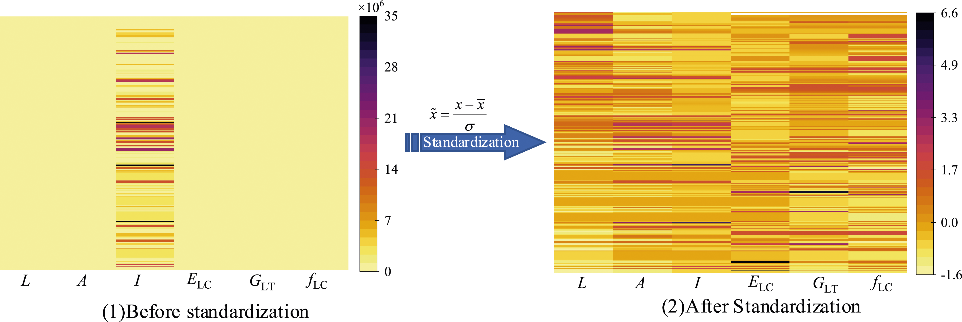$\bar{x}$ is the mean of the feature data, and $σ$ is the standard deviation of the feature data.

Evaluation of indicators and optimization of hyperparameters

Evaluation metrics of models

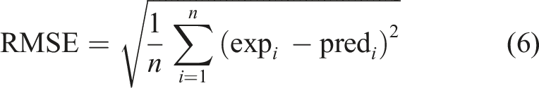
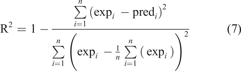
To evaluate the performance of the learning machines proposed to predict the buckling critical loads, widely used indicators have been used, including standard deviation (STD), mean squared error (MSE), root-mean-squared error (RMSE), and correlation coefficient (R²). Their related equations (4)–(6) are, respectively, as follows: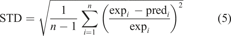

STD = \sqrt{\frac{1}{n - 1} \sum_{i = 1}^{n} {(\frac{\exp_{i} - {pred}_{i}}{\exp_{i}})}^{2}}

(5)

RMSE = \sqrt{\frac{1}{n} \sum_{i = 1}^{n} {(\exp_{i} - {pred}_{i})}^{2}}

(6)

R^{2} = 1 - \frac{\sum_{i = 1}^{n} {(\exp_{i} - {pred}_{i})}^{2}}{\sum_{i = 1}^{n} {(\exp_{i} - \frac{1}{n} \sum_{i = 1}^{n} (\exp_{i}))}^{2}}

(7)

where

n

is the number of specimens, while

\exp_{i}

and

{pred}_{i}

are the buckling critical loads of experimental specimens and those predicted by learning machines, respectively.

Hyperparameters optimization

In this paper, we use the experimental database in Table 1 to train machine learning models for hyperparameter optimization. The dataset is randomly sampled in the ratio of 2:8 into a training dataset (292 sets) and a testing dataset (73 sets). The random sampling division largely eliminates the effect of correlation between data on the training results. For the reconstruction ability of machine learning models, the random seed is set to ensure the consistency of the reconstructed model each time. Due to the randomness of the training set division, the training error at one time usually does not represent the generalization error of the model. To eliminate this randomness, reduce the sensitivity of the model to different training sets, and obtain a model with better generalization performance, a 10-fold cross-validation model, which is a k-fold cross-validation, is adopted. Selecting model parameters through cross-validation is more stable and comprehensive than dividing the training and testing datasets at once.

In order to enhance the models’ accuracy, this paper adopts a variety of optimization algorithms in determining the hyperparameters, with optimized curves, optimized surfaces, grid search, and random search. The specific optimization process is as follows:

(1) Hyperparameters of support vector regression model

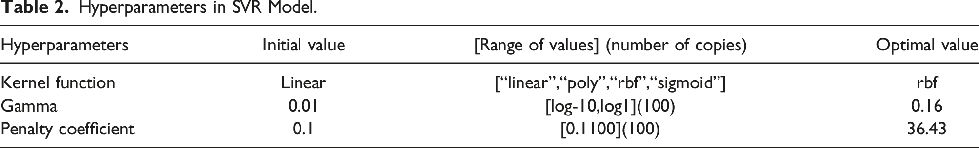
The hyperparameters of the support vector regression algorithm are mainly calculated by optimizing the curve. Firstly, the kernel function is optimized, and the radial basis kernel function has the highest goodness of fit, see Figure 7(a); after determining the kernel function, the gamma parameter is optimized, as shown in Figure 7(b), and the goodness of fit is the highest when gamma = 0.16; in the case of the radial basis kernel function and gamma = 0.16, the penalty coefficients are optimized, as shown in Figure 7(b), and the goodness of fit is the highest when the penalty coefficient = 36.34, the best fit is obtained. Finally, the best-fitting hyperparametric model can be obtained, and the optimal values of hyperparameters are shown in Table 2.

Figure 7.

SVR hyperparameter optimization curve, (a) Preference of kernel function, (b) Optimization of gamma parameters and the penalty coefficient.

Table 2.

Hyperparameters in SVR Model.

Hyperparameters	Initial value	[Range of values] (number of copies)	Optimal value
Kernel function	Linear	[“linear”,“poly”,“rbf”,“sigmoid”]	rbf
Gamma	0.01	[log-10,log1](100)	0.16
Penalty coefficient	0.1	[0.1100](100)	36.43

(2)Hyperparameters of extreme gradient boosting model

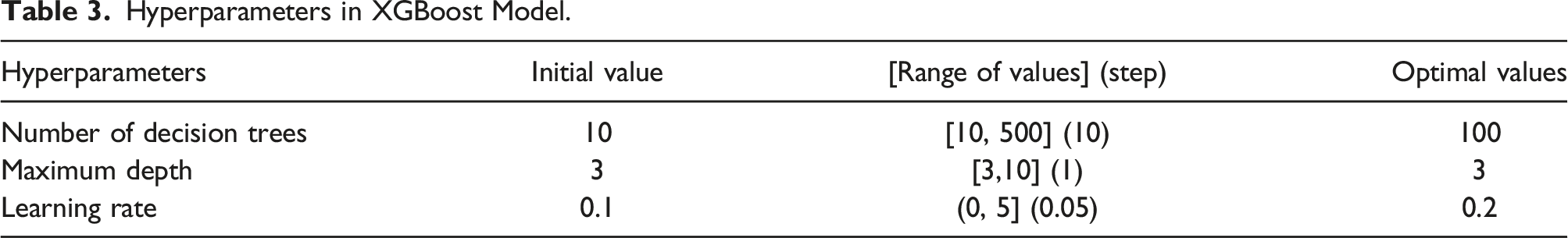
In the XGBoost algorithm model, the first hyperparameters to be determined are the number of decision trees and the maximum depth of decision trees. The number and depth of the decision tree interact with each other; the fitting effect can be improved by increasing the number of the decision tree, and the fitting effect can also be improved by increasing the depth of the decision tree, and at the same time, these two practices are also prone to overfitting, so it is necessary to set these two parameters jointly and coordinately to prevent the occurrence of overfitting. The cloud plot of the goodness-of-fit after two-parameter optimization is shown in Figure 8(a).

Figure 8.

Hyperparameters optimization of XGBoost model, (a) Optimization of the number of decision trees and decision tree depth (b) Optimization of the learning rate.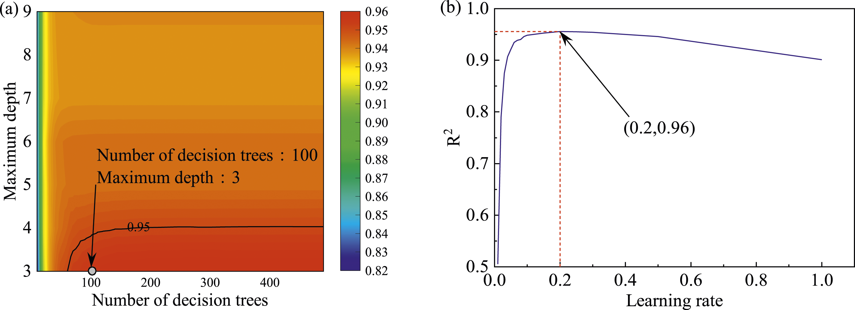

The number of decision trees and the maximum depth of the decision tree are combined in more ways within the contour line with goodness of fit equal to 0.95. Considering the computation speed, the number of decision trees and the maximum depth of decision trees are as small as possible. Hence, the number of decision trees is 100, and the maximum depth of decision trees is 3. In addition, the learning rate needs to be specified, also known as the step size of the decision tree iteration. The larger the learning rate, the faster the iteration speed, and the faster the limit can be reached, but it is possible to miss the real best value. The smaller the learning rate, the slower the iteration speed and the more likely to find the exact best value. The optimization curve for the learning rate in Figure 8(b) shows that the best fit is achieved when the learning rate is 0.2. The optimal hyperparameter values for the final model are shown in Table 3.

Table 3.

Hyperparameters in XGBoost Model.

Hyperparameters	Initial value	[Range of values] (step)	Optimal values
Number of decision trees	10	[10, 500] (10)	100
Maximum depth	3	[3,10] (1)	3
Learning rate	0.1	(0, 5] (0.05)	0.2

(3)Hyperparameters of artificial neural network model

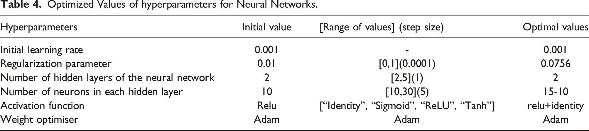
The activation function of an artificial neuron is the core parameter of the neural network structure. Therefore, the activation function is the first hyperparameter to be determined. For the regression prediction problem, the activation function of the output layer is usually chosen as a constant function, that is, the Identity function, and thus, the activation function of the hidden layer is the hyperparameter to be determined. For the neural network structure in this paper, the number of neurons in the input layer is the number of features in the training sample six. The number of neurons in the output layer is the number of prediction targets 1, but the number of hidden layers and neurons in each layer still needs to be determined. In addition to this, for the artificial neural network machine learning model, the hyperparameters that need to be determined are the weight optimizer, the initial learning rate to control the update weight compensation, and the regularization parameter to prevent overfitting. Among them, the default adaptive optimizer, Adam, is chosen for the weight optimizer, which automatically adjusts the learning rate during the training process, and the initial learning rate can be optionally set. Due to the large number of neural network hyperparameters and their interaction, the optimal hyperparameter values cannot be obtained for the optimization curve or surface.

In this paper, a combination of grid search and random search is used to optimize the hyperparameters. The optimal values of the optimized hyperparameters are shown in Table 4.

Table 4.

Optimized Values of hyperparameters for Neural Networks.

Hyperparameters	Initial value	[Range of values] (step size)	Optimal values
Initial learning rate	0.001	-	0.001
Regularization parameter	0.01	[0,1](0.0001)	0.0756
Number of hidden layers of the neural network	2	[2,5](1)	2
Number of neurons in each hidden layer	10	[10,30](5)	15-10
Activation function	Relu	[“Identity”, “Sigmoid”, “ReLU”, “Tanh”]	relu+identity
Weight optimiser	Adam	Adam	Adam

The structure of the optimal artificial neural network model trained to be used for prediction is shown in Figure 9.

Figure 9.

Artificial neural network structure.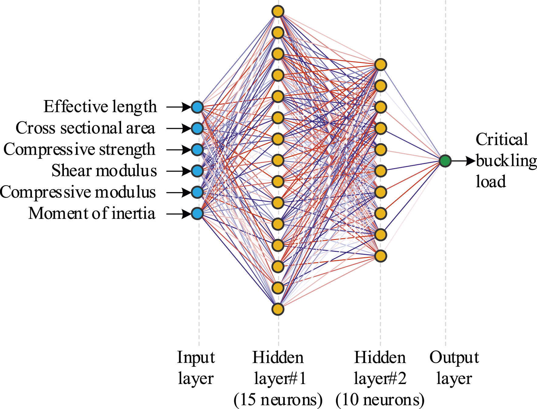

Results and discussion

Performance evaluation of machine learning models

Evaluation of prediction accuracy

In Figures 10 –12, the machine learning model prediction results are compared with the experimental results. As shown in the figures, all three machine learning models, XGBoost, SVR, and ANN, obtained high $R^{2}$ values for the training dataset, 0.99, 0.97, and 0.98, respectively, indicating that all three models have sound fitting effects. The high $R^{2}$ values of 0.96, 0.96, and 0.97 are also achieved for the testing dataset, indicating that the three machine learning models also have good generalization ability. Furthermore, the $R^{2}$ values for the training and the testing datasets are almost equal, indicating that the models are not overfitted or underfitted.

Figure 10.

XGBoost predictions versus experimental results, (a) The training dataset, (b) The testing dataset, (c) The entire dataset.

Figure 11.

SVR model predicted results versus experimental results, (a) The training dataset, (b) The testing dataset, (c) The entire dataset.

Figure 12.

ANN model predicted results versus experimental results, (a) The training dataset, (b) The testing dataset, (c) The entire dataset.

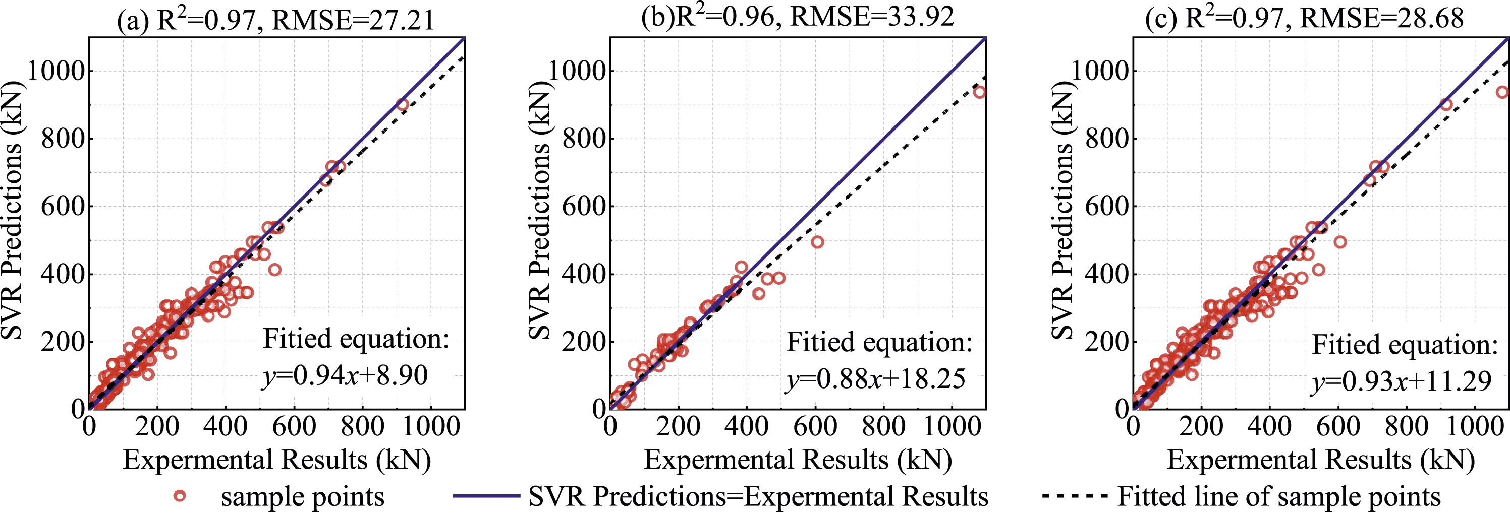
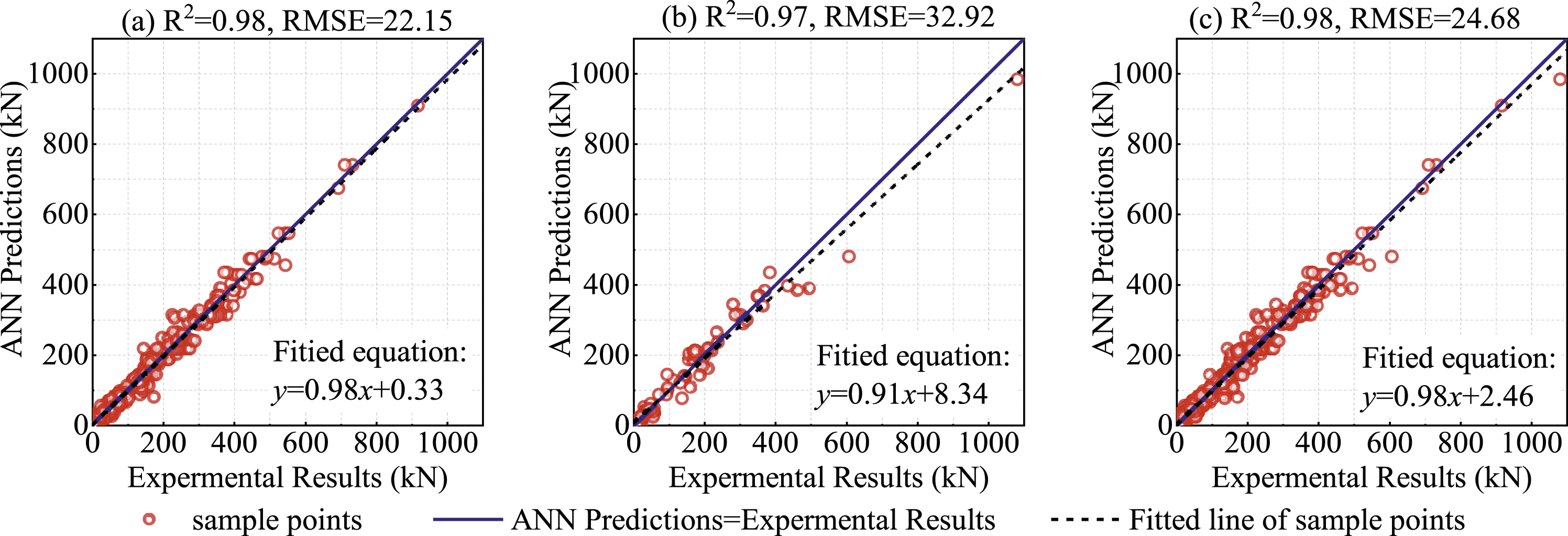
For the entire datasets, all models demonstrated a high capability of predicting the flexural buckling critical load of pultruded FRP struts. The XGBoost and ANN models achieved slightly better performance compared to the SVR.

Evaluation of prediction stability

The prediction error counts of the XGBoost, SVR, and ANN models are counted separately, which further reflects the accuracy and stability of the prediction results, as shown in Figure 13. The yellow area in the figure indicates the count of prediction errors on the training set, and the blue area indicates the count of prediction errors on the test set. The two are superimposed together to represent the prediction error counts on the entire dataset. The closer the prediction error is to the zero error, the higher the prediction accuracy is. As can be seen in the figure, the three machine learning models have the largest number of samples with prediction errors concentrated near zero error, indicating that the predicted values of the models are consistent with the actual values and the prediction accuracy is high.

Figure 13.

Error frequency count of models: (a) XGBoost model, (b) SVR model, (c) ANN model. Note. Prediction error = prediction value-experimental value.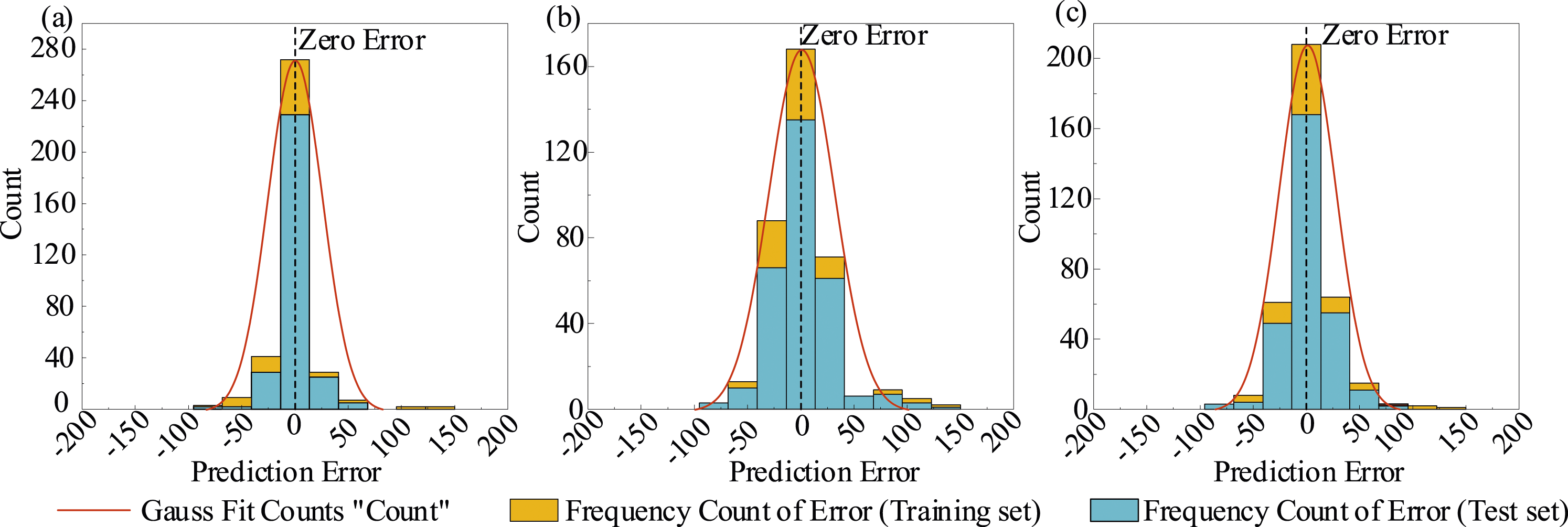

Figure 13 displays the error frequency counts of the model on the training and test sets fitted with a Gaussian curve. The graph shows that the distribution of prediction error counts conforms to the normal distribution with zero mean, the sample distribution of the zero error add-on distribution is the largest, and the sample distribution decreases with the error increase. The fact that the prediction results conform to the normal distribution indicates that the model is relatively stable. The predicted values of the model are consistent with the actual values, and the regression prediction target is well accomplished.

Comparison of prediction results with traditional algorithms

Euler’s critical load prediction method (equation (1)), Engesser’s theory-based shear-modified critical load prediction method (equation (3)), and Ayrton-Perry’s formula based on the edge yielding criterion (equation (4)) are the commonly used classical and conventional critical load prediction algorithms for buckling.

As mentioned in the introduction, no fixed form of the polynomial equation fits in the regression fitting of Perry’s formula. Therefore, the fitting relationship between the equivalent initial bending curvature and the regularized slenderness ratio needs to be optimized when using the Perry formula for prediction, and the optimization method is referred to in the literature (Zhang and Li, 2024). By optimization, the equivalent initial bending curvature of pultruded FRP members is fitted by a quadratic trinomial $ε_{0} = 0.1805 λ_{n}^{2} - 0.2687 λ_{n} + 0.2206$ .

Predicted results of traditional algorithms

In the entire dataset, as shown in Figure 14, the $R^{2}$ values of the prediction results of Euler’s formula, Engesser’s shear correction formula, and Ayrton-Perry formula are 0.75, 0.90, and 0.94, respectively. It indicates that the prediction accuracy of the Ayrton-Perry formula is better than that of Engesser’s shear correction formula, and the prediction accuracy of Euler’s formula is the poorest. This is mainly because the Euler formula is established based on the Euler-Bernoulli assumption, neglecting to consider the shear deformation and initial defects. Compared with Euler’s formula, the prediction accuracy of Engesser’s shear correction formula is greatly improved, mainly because Engesser’s shear correction formula considers shear deformation. It also indicates that the effect of shear deformation on the critical buckling load of pultruded FRP columns is significant and cannot be neglected. The Ayrton-Perry formula critical load prediction method is based on the regression of experimental results. It implicitly considers shear deformation and initial defects, so it has the highest prediction accuracy among the traditional theoretical methods. However, the improvement in the $R^{2}$ value of Ayrton-Perry formula prediction results is only 4% relative to Engesser’s shear correction formula. This suggests that the pultruded FRP columns in the database, which were collected in this paper, are nearly perfect with only minor initial defects. Hence, these defects have a lesser impact on the critical load.

Figure 14.

The predicted results by traditional algorithm versus experimental results, (a) Euler formula predicted results, (b) Engesser’s shear correction formula predicted results, (c)Ayrton-Perry formula predicted results.

Predicted results of machine learning algorithms versus traditional algorithms

Comparing Figure 14 with Figures 10 –12, respectively, it can be seen that the prediction accuracy of traditional theoretical methods is lower than that of machine learning algorithms. In addition, the distribution of sample points in Figure 14 is skewed towards the upper line of equal value and is discrete, indicating that the prediction results of traditional theoretical algorithms are always large and discrete. In contrast, the distribution of sample points in Figures 10 –12 is balanced between left and right, suggesting that the machine learning algorithm is more stable. The fitted lines for the sample points in Figure 14 are significantly above the line of equal value, indicating that the traditional theoretical model predictions are generally greater than the experimental results, which is unsafe for the design. In contrast, the fitted lines of the sample points in Figures 10 –12 are all below the line of equal value, indicating that the machine learning model predictions are generally smaller than the experimental results, which is safe for the design.

To compare the machine learning models with the traditional algorithms more comprehensively, a Taylor diagram is plotted, as shown in Figure 15. The Taylor diagram graphically summarizes how close a pattern (or set of patterns) is to the base values. The similarities between these patterns are expressed by comparing and quantifying their correlation values, their centered root-mean-square error, and their standard deviation by this graph (Mousavi et al., 2023).

Figure 15.

Taylor diagram for comparison performance of the machine learning methods and existing models in terms of predicting buckling critical load of pultruded FRP columns.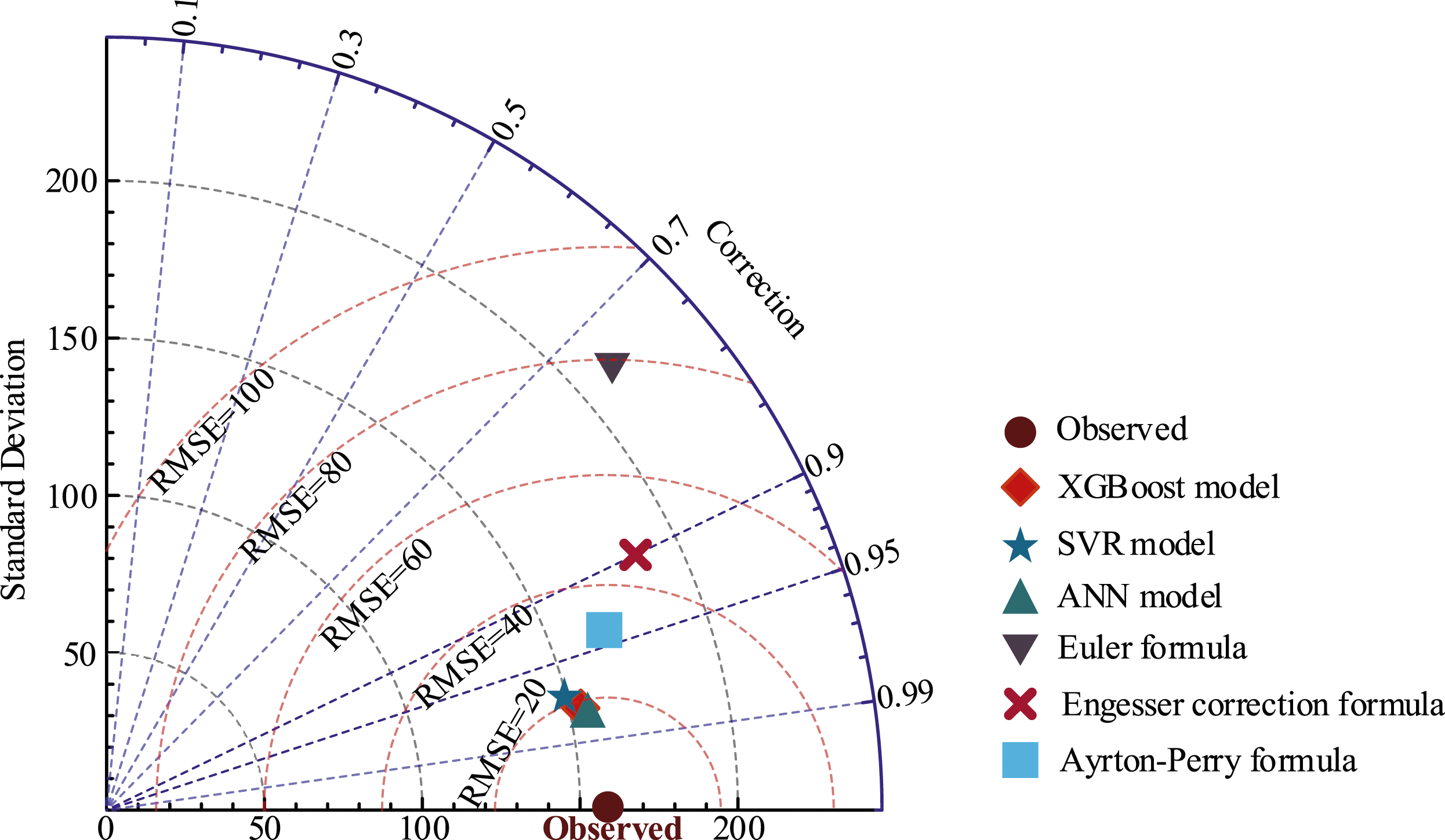

As shown in Figure 15, in general, machine learning methods, in addition to the highest R² coefficient, have had the lowest standard deviation and the closest value of RMSE compared to the models in predicting the buckling critical loads. In the machine learning methods proposed in this regard, ANN, SVR, and XGBoost performed the best, respectively. However, there was a slight difference between the three machine learning methods in R² coefficient and RMSE error values; the Taylor diagram shows that the standard deviation of all three machine learning methods is closer to the experimental values. These results suggest that traditional theoretical methods have significant errors and do not perform satisfactorily when facing large datasets. However, machine learning methods have been able, through their artificial intelligence and creating inter-data links, to provide extremely accurate predictions of the buckling critical loads of FRP struts, even with large datasets.

Feature interpretation and analysis

When it comes to machine learning models, they are often considered “black box models” that are difficult to explain. However, the Shapley Additive Explanations (SHAP) algorithm has been developed to help with this issue. SHAP is an ex-post algorithm that can explain machine learning models by calculating the impact of each feature on the model’s output (Zhang et al., 2022). This algorithm can be used globally and locally, and all features are considered “contributors”. For each prediction sample, the model generates a prediction value, and the SHAP value is assigned to each feature in that sample. Furthermore, this algorithm can cover almost all machine learning models.

Summarize the effects of all the features

For the three machine learning models, the SHAP values of each input feature on the output results are embodied in Figure 16. In those figures, each line in the figure represents a feature, and the horizontal coordinates are the SHAP values. The features are ordered by the average absolute value of SHAP. A broad area indicates a large number of samples aggregated. Each point is a sample, and the color from blue to red represents the increasing eigenvalues.

Figure 16.

Feature importance analysis using SHAP value, (a) XGBoost model, (b) SVR model, (3) ANN model.

The order of input variable effect on prediction accuracy of all machine learning models can be sorted by descending: moment of inertia > effective length > cross-sectional area > compressive modulus > shear modulus > compressive strength. Although the importance of various features in the machine learning models is slightly different due to different algorithms, the features with the greatest and the least impact and the order of arrangement are the same.

Importance analysis

The importance of features is usually measured by calculating the average absolute value of SHAP values for each feature. However, it may be challenging to directly compare the feature importance values of different models. Therefore, the relative importance of each feature of a model can be characterized by the percentage of each feature relative to the overall feature importance of the model. This approach calculates the percentage of a feature importance value of a model relative to the sum of all feature importance values of that model. For example, in Figure 17, the contribution of the moment of inertia to the prediction of the buckling critical load in the XGBoost model accounts for 52% of the overall feature contribution. In this way, we can compare the relative importance of features in different models without directly comparing their importance values. This can help us to understand better which features in each model have a more significant impact on the final results.

Figure 17.

Relative importance of features.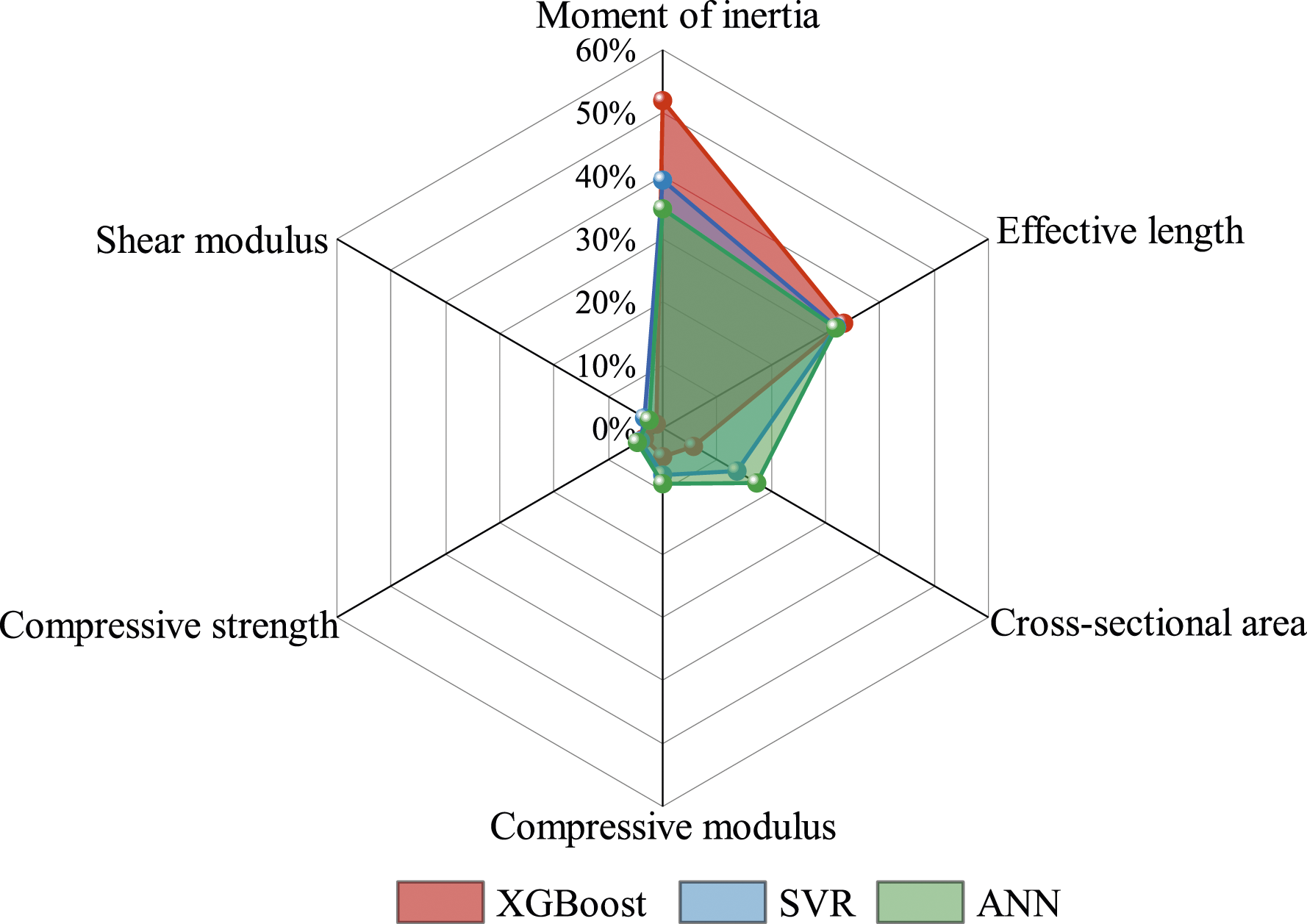

It can be seen from Figure 17 that the geometric parameters (effective length, cross-section area, moment of inertia) contribute significantly to the contribution of the critical load, more than 80%. The contribution of the material parameters (compressive modulus, shear modulus, compressive strength) to the critical load is small, at most 20%. This also verifies that the bending buckling problem is a geometric abrupt change problem, not a strength problem of material control.

Correlation analysis

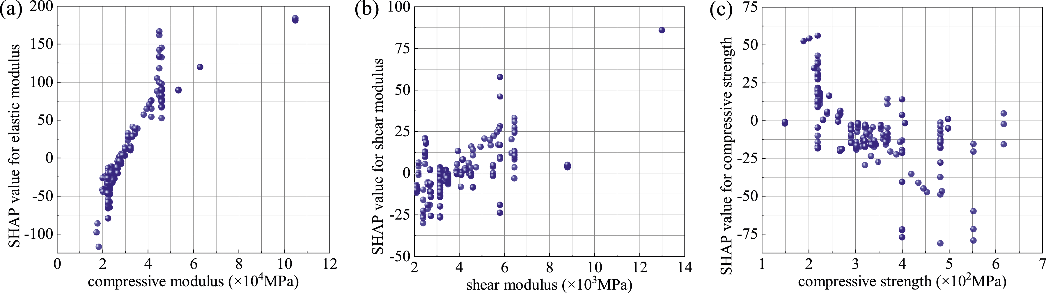
The SHAP partial dependence plot shows the marginal effect of individual features on the predicted outcome of a machine learning model, and it can show whether the relationship between the target and the features is linear, monotonic, or more complex. Taking the ANN model as an example, the effect of geometric and material parameters on the critical load is analyzed separately using SHAP local dependence plots, as shown in Figures 18 and 19.

Figure 18.

Effect of geometric parameters on prediction results, (a) effective length, (b) cross-section area, (c) moment of inertia.

Figure 19.

Effect of material parameters on prediction results, (a) compressive modulus, (b) shear modulus, (c) compressive strength.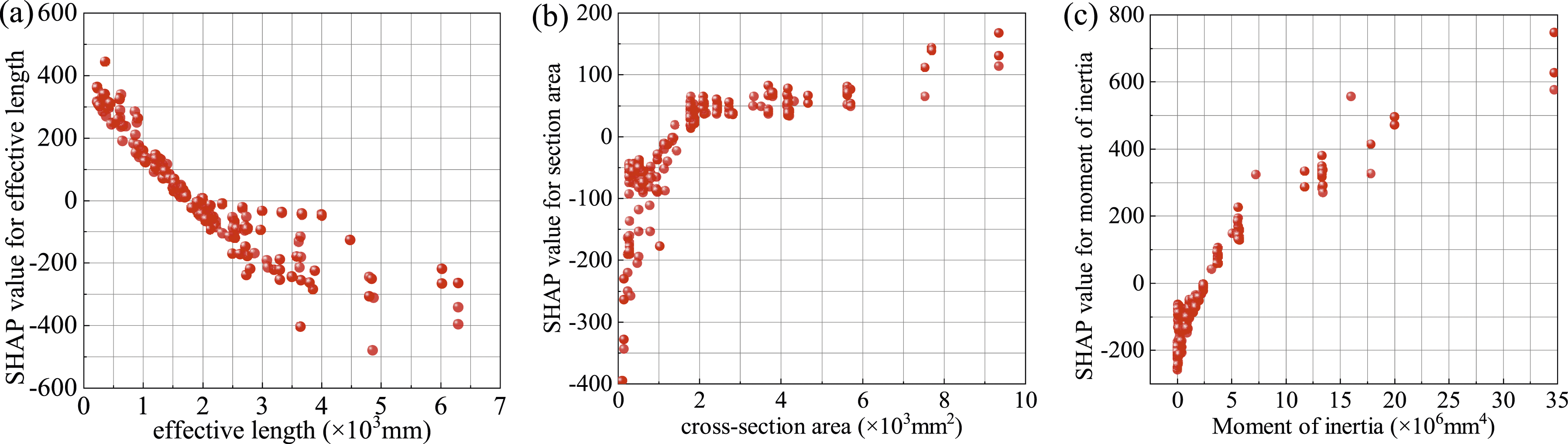

As shown in Figure 18, the SHAP value shows that cross-section area and moment of inertia have a non-linear positive correlation with the flexural critical load of the pultruded FRP members. At the same time, the effective length is a relatively obvious non-linear negative correlation.

As shown in Figure 19, the SHAP value shows that compressive modulus has a relatively obvious positive correlation with the flexural critical load of the pultruded FRP member. In contrast, the shear modulus and compressive strength have no obvious correlation.

Conclusion

In this paper, a method for predicting the buckling critical load of Pultruded FRP columns is established by a machine learning model. By analyzing the prediction accuracy of the model, the stability of the prediction, and the importance of the features, the following conclusions are as follows:

(1) Machine learning methods have excellent prediction performance. Among them, the ANN model (R² = 0.97, RMSE = 32.92) has the best prediction performance. While the prediction performance of XGBoost (R² = 0.96, RMSE = 37.08) is worse, it is also much higher than the prediction performance of the most commonly used Euler’s formula (R² = 0.75, RMSE = 78.66), and slightly higher than Perry’s formula (R2 = 0.94, RMSE = 39.82), which has the best prediction performance among the traditional theoretical methods. Although both the machine learning method and Perry’s formula are based on experimental data for regression prediction, the machine learning method solves the problem of uncertainty in fitting experimental data in the use of Perry’s formula.

(2) The impact of six input characteristics (moment of inertia, effective length, cross-sectional area, compressive modulus, shear modulus, compressive strength) on the buckling critical load of pultruded FRP columns is well analyzed through the SHAP value. Although the importance of various features in the machine learning models is slightly different due to different algorithms, the features with the greatest and the least impact and the order of arrangement are the same. The order of input variable effect on prediction accuracy of all machine learning models can be sorted by descending: moment of inertia > effective length > cross-sectional area > compressive modulus > shear modulus > compressive strength. The effect of the moment of inertia is the most obvious, while the effects of shear modulus and compressive strength are small.

(3) The contribution of geometric and material parameters to the buckling critical load is quantified by the feature analysis. The contribution of geometric parameters (effective length, cross-section area, moment of inertia) is more than 80%. Meanwhile, the contribution of material parameters (compressive modulus, shear modulus, compressive strength) is small, less than 20%.

(4) Thorough analysis of the SHAP Partial dependence plot shows that the buckling critical load of pultruded FRP members has a nonlinear positive correlation with the cross-sectional area, the moment of inertia, and compression modulus, and a significant nonlinear negative correlation with effective length, while no significant correlation with shear modulus and compressive strength.

Footnotes

Declaration of conflicting interests

The author(s) declared no potential conflicts of interest with respect to the research, authorship, and/or publication of this article.

Funding

The author(s) disclosed receipt of the following financial support for the research, authorship, and/or publication of this article: This study is supported by. National Natural Science Foundation of China No (52278288).

ORCID iD

Feng Li

References

Bank LC (2006) Composites for Construction: Structural Design with FRP Materials. Hoboken, N.J: John Wiley & Sons.

Barbero

Raftoyiannis

(1993) Euler buckling of pultruted composite columns. Composite Structures 24: 139–147. DOI: 10.1016/0263-8223(93)90035-O

Barbero

Tomblin

(1993) Euler buckling of thin-walled composite columns. Thin-Walled Structures 17: 237–258. DOI: 10.1016/0263-8231(93)90005-U

Blandford

(2010) Critical Buckling Strength Prediction of Pultruded GFRP Composite Columns. Morgantown: MS. West Virginia University Libraries, DOI: 10.33915/etd.2279

Boscato

Casalegno

Russo

, et al. (2014) Buckling of built-up columns of pultruded fiber-reinforced polymer C-sections. Journal of Composites for Construction 18: 04013050. DOI: 10.1061/(ASCE)CC.1943-5614.0000453

Boscato

Casalegno

Russo

(2015) Performance of built-up columns made by pultruded FRP material. Composite Structures 121: 46–63. DOI: 10.1016/j.compstruct.2014.11.022

Cardoso

DCT

Harries

Batista

Ede M

(2014) Compressive strength equation for GFRP square tube columns. Composites Part B: Engineering 59: 1–11. DOI: 10.1016/j.compositesb.2013.10.057

Ding

Liu

Wang

, et al. (2018) Mechanical properties of pultruded basalt fiber-reinforced polymer tube under axial tension and compression. Construction and Building Materials 176: 629–637. DOI: 10.1016/j.conbuildmat.2018.05.036

Feng

Qian

(2008) Analysis of Global Buckling of FRP Pipes under Axial Compression.

10.

Feng

Chen

Cui

, et al. (2021) Critical loads of axially compressed GFRP round tubes considering shear deformations. Journal of Zhejiang University (Engineering Science) 55: 1894–1902. DOI: 10.3785/j.issn.1008-973X.2021.10.011

11.

Feng

Liu

(2022) Non-uniform fiber-resin distributions of pultruded GFRP profiles. Composites Part B: Engineering 231: 109543. DOI: 10.1016/j.compositesb.2021.109543

12.

Goodman

Gliksman

(1969) Structural Evaluation of Long Boron Composite Columns. PA, USA. ASTM International, 460. DOI: 10.1520/STP49835S

13.

Hashem

Yuan

(2001) Short vs. long column behavior of pultruded glass-fiber reinforced polymer composites. Construction and Building Materials 15: 369–378. DOI: 10.1016/S0950-0618(01)00018-6

14.

Hewson

(1978) Buckling of pultruded glass fibre-reinforced channel sections. Composites 9: 56–60. DOI: 10.1016/0010-4361(78)90520-7

15.

Higgoda

Elchalakani

Kimiaei

, et al. (2023a) Experimental investigation on the structural behaviour of novel non-metallic pultruded circular tubular GFRP T-joints under axial compression. Thin-Walled Structures 184: 110512. DOI: 10.1016/j.tws.2022.110512

16.

Higgoda

Elchalakani

Kimiaei

, et al. (2023b) Experimental and numerical investigation of pultruded GFRP circular hollow tubular columns under concentric and eccentric loading. Composite Structures 304: 116427. DOI: 10.1016/j.compstruct.2022.116427

17.

Hou

Zhang

Feng

(2010) Stability of axial compression members of glass fober-reinforced plastic(GFRP). Journal of Building Materials 13: 441.

18.

Iyengar

NGR

(1988) Structural Stability of Columns and Plates. Chichester: John Wiley & Sons.

19.

Jerath

(2021) Structural Stability Theory and Practice: Buckling of Columns, Beams, Plates, and Shells. Hoboken: Wiley.

20.

Kardomateas

Dancila

(1997) Buckling of moderately thick orthotropic columns: comparison of an elasticity solution with the Euler and Engesser/Haringx/Timoshenko formulae. International Journal of Solids and Structures 34: 341–357. DOI: 10.1016/S0020-7683(96)00020-0

21.

Kumar

Yadav

(2013) Buckling analysis of a beam–column using multilayer perceptron neural network technique. Journal of the Franklin Institute 350: 3188–3204. DOI: 10.1016/j.jfranklin.2013.07.016

22.

Lane

Mottram

(2002) Influence of modal coupling on the buckling of concentrically loaded pultruded fibre-reinforced plastic columns. Proceedings of the Institution of Mechanical Engineers, Part L: Journal of Materials: Design and Applications 216: 133–144. DOI: 10.1177/146442070221600208

23.

Lee

Hewson

(1979) The use of fibre-reinforced plastics in thin-walled structures. Conf Stress Anal Group Inst Phys 1978: 23–55.

24.

(2019) Study on Glass Fiber Reinforced Composite Axial Compression Members. Master. Nanjing, China. Nanjing University of Science and Technology.

25.

Zhu

(2020) Overall buckling prediction model for fibre reinforced plastic laminated tubes with balanced off-axis ply orientations based on Puck failure criteria. Journal of Composite Materials 54: 883–897. DOI: 10.1177/0021998319871086

26.

Zhu

(2021) Axial compression performance of pultruded GFRP tube based on casing buckling restraint. Acta Materiae Compositae Sinica 38: 3255–3269. DOI: 10.13801/j.cnki.fhclxb.20201222.002

27.

Liu

(2020) Experimental and Theoretical Study on the Stability of Pultruded GFRP Axial Compression Members. Master. Nanjing, China. Nanjing University of Science and Technology.

28.

Monteiro

ACL

Malite

(2021) Behavior and design of concentric and eccentrically loaded pultruded GFRP angle columns. Thin-Walled Structures 161: 107428. DOI: 10.1016/j.tws.2020.107428

29.

Mottram

Brown

Anderson

(2003) Physical testing for concentrically loaded columns of pultruded glass fibre reinforced plastic profile. Proceedings of the Institution of Civil Engineers - Structures and Buildings 156: 205–219. DOI: 10.1680/stbu.2003.156.2.205

30.

Mousavi

Bahr Peyma

Mousavi

, et al. (2023) Predicting the ultimate and relative bond strength of corroded bars and surrounding concrete by considering the effect of transverse rebar using machine learning. Iran J Sci Technol Trans Civ Eng 47: 193–219. DOI: 10.1007/s40996-022-00909-7

31.

Mukherjee

Deshpande

Anmala

(1996) Prediction of buckling load of columns using artificial neural networks. Journal of Structural Engineering 122: 1385. DOI: 10.1061/(ASCE)0733-9445(1996)122:11(1385)

32.

Nguyen

T-H

Tran

N-L

Nguyen

D-D

(2021) Prediction of critical buckling load of web tapered I-section steel columns using artificial neural networks. Int J Steel Struct 21: 1159–1181. DOI: 10.1007/s13296-021-00498-7

33.

Nunes

Correia

, et al. (2013) Experimental and numerical study on the structural behavior of eccentrically loaded GFRP columns. Thin-Walled Structures 72: 175–187. DOI: 10.1016/j.tws.2013.07.002

34.

Nunes

Correia

Silvestre

(2016) Structural behaviour of hybrid FRP pultruded columns. Part 1: experimental study. Composite Structures 139: 291–303. DOI: 10.1016/j.compstruct.2015.12.058

35.

Pacheco

Sá

Correia

, et al. (2021) Structural safety of pultruded FRP profiles for global buckling. Part 2: reliability-based evaluation of safety formats and partial factor calibration. Composite Structures 257: 113147. DOI: 10.1016/j.compstruct.2020.113147

36.

Puente

Insausti

Azkune

(2006) Buckling of GFRP columns: an empirical approach to design. Journal of Composites for Construction 10: 529–537. DOI: 10.1061/(ASCE)1090-0268(2006)10:6(529)

37.

Roberts

(2002) Influence of shear deformation on buckling of pultruded fiber reinforced plastic profiles. Journal of Composites for Construction 6: 241. DOI: 10.1061/(ASCE)1090-0268(2002)6:4(241)

38.

Sá

Pacheco

Correia

, et al. (2021) Structural safety of pultruded FRP profiles for global buckling. Part 1: approach to material uncertainty, resistance models, and model uncertainties. Composite Structures 257: 113304. DOI: 10.1016/j.compstruct.2020.113304

39.

Seangatith

Sriboonlue

(1999) Axially-loaded glass-fiber reinforced plastic composite columns. Kochi, Japan: 1307–1312.

40.

Sheidaii

Bahraminejad

(2012) Evaluation of compression member buckling and post-buckling behavior using artificial neural network. Journal of Constructional Steel Research 70: 71. DOI: 10.1016/j.jcsr.2011.10.020

41.

Sun

(2018) Experimental and Theoretical Research on Carbon Fiber Reinforced Composite Axial Compression Members. Master. Nanjing, China. Nanjing University of Science and Technology.

42.

Thai

H-T

(2022) Machine learning for structural engineering: a state-of-the-art review. Structures 38: 448–491. DOI: 10.1016/j.istruc.2022.02.003

43.

Vanevenhoven

Shield

Bank

(2010) LRFD factors for pultruded wide-flange columns. Journal of Structural Engineering 136: 554–564. DOI: 10.1061/(ASCE)ST.1943-541X.0000126

44.

Wang

Zhao

(2011) Stability analysis of axial compression component of FRP. Electric Power Construction 32: 85–89, (in chinese).

45.

Wang

Shun

, et al. (2016) Experimental and theoretical study on ultimate bearing capacity of GFRP tubes under axial compression. Journal of Building Materials 19: 1033.

46.

Tian

Ding

, et al. (2022) Axial compression behavior of pultruded GFRP channel sections. Composite Structures 289: 115438. DOI: 10.1016/j.compstruct.2022.115438

47.

Xie

Bai

, et al. (2019) Pultruded GFRP square hollow columns with bolted sleeve joints under eccentric compression. Composites Part B: Engineering 162: 274–282. DOI: 10.1016/j.compositesb.2018.11.001

48.

Sun

Wang

, et al. (2013) Experimental and theoretical study on stability of slender components made from glass fiber/expoxy composite material. Engineering Mechanics 30: 251.

49.

Zheng

Zhang

(2021) Capacity prediction of cold-formed stainless steel tubular columns using machine learning methods. Journal of Constructional Steel Research 182: 106682. DOI: 10.1016/j.jcsr.2021.106682

50.

Zhan

(2018a) Global buckling capacity of pultruded FRP-I section columns under axial compression. Mechanics Research Communications 90: 8–17. DOI: 10.1016/j.mechrescom.2018.04.002

51.

Zhan

(2018b) Determination of critical loads for global buckling of axially loaded pultruded fiber-reinforced polymer members with doubly symmetric cross sections. Advances in Structural Engineering 21: 1911–1922. DOI: 10.1177/1369433218759572

52.

Zhan

Harries

(2018) Determination of critical load for global flexural buckling in concentrically loaded pultruded FRP structural struts. Engineering Structures 158: 1–12. DOI: 10.1016/j.engstruct.2017.12.008

53.

Zhang

(2019) Study on the Stability of Carbon Fiber Reinforced Composite Axial Compression Bar. Master. Nanjing, China. Nanjing University of Science and Technology.

54.

Zhang

(2024) A review of prediction methods for global buckling critical loads of pultruded FRP struts. Composite Structures 329: 117752. DOI: 10.1016/j.compstruct.2023.117752

55.

Zhang

Feng

(2011) Experimental research of fiber reinforced plastics equal angle axial compression members. Fiber Reinforced Plastics/Composites: 51–54.

56.

Zhang

Liu

Feng

(2014) Stable performance of FRP tube axial compression members. Fiber Reinforced Plastics/Composites: 19–22.

57.

Zhang

Niu

Yang

, et al. (2022) Machine learning prediction models for compressive strength of calcined sludge-cement composites. Construction and Building Materials 346: 128442. DOI: 10.1016/j.conbuildmat.2022.128442

58.

Zureick

Scott

(1997) Short-term behavior and design of fiber-reinforced polymeric slender members under axial compression. Journal of Composites for Construction 1: 140. DOI: 10.1061/(ASCE)1090-0268(1997)1:4(140)

59.

Zureick

Steffen

(2000) Behavior and design of concentrically loaded pultruded angle struts. Journal of Structural Engineering 126: 406–416. DOI: 10.1061/(ASCE)0733-9445(2000)126:3(406)