Linear and nonlinear time-series methodologies for bridge condition assessment: A literature review

Abstract

Railway bridges are essential components of any transportation system and are typically subjected to several environmental and operational actions that can cause damage. Furthermore, they are not easily replaced, and their failure can have catastrophic consequences. Considering the expected lifespan of bridges, it is essential to guarantee their adequate serviceability and safety. In this scenario, emerges the Structural Health Monitoring (SHM), which allows the early identification of damage before it becomes critical. Damage identification is usually performed by the comparison between the damaged and undamaged responses obtained from monitoring data. Among the several features extracted from the responses, the time-series models exhibit a better performance, capability of early damage detection, and may also be applied within online damage detection strategies using unsupervised machine learning frameworks. In this paper, a review of advanced time-series methodologies for damage detection is presented. Initially, several time-series models often used in SHM are described, such as Autoregressive Models (AR), Recurrent Neural Networks (RNN), Gated Recurrent Unit (GRU), and Long Short-Term Memory (LSTM). Later, the framework where these models are usually applied is also detailed, including the latest upgrades and most relevant results. Finally, the conclusions summarize and elucidate the current perspectives and research gaps on the time-series models.

Keywords

structural health monitoring railway bridges condition assessment damage detection linear time-series models nonlinear time-series models

Introduction

The railway network infrastructure plays a vital role by connecting different regions and allowing services and goods to be transported. Railway bridges are critical components on these large-scale transportation systems that require permanent attention by infrastructure managers (Azim, 2021; Chalouhi et al., 2017). During their large life cycle, these structures might change both traffic and environmental load conditions as well as materials properties. For the former, it must be pointed the increasing traffic volume, vehicle speed, and axle loads, as well as extreme temperature changes or even the occurrence of exceptional events. For the latter, it should be referred to the often-observed degradation processes associated with corrosion and fatigue (Chalouhi et al., 2017; Matsuoka et al., 2021). Hence, Structural Health Monitoring (SHM) systems for the condition assessment of railway bridges have been widely documented as a tool to ensure an adequate structural performance during the structure’s life cycle based on safety and economic criteria.

In recent SHM systems, the condition assessment involves measuring the structural responses under traffic/environmental loads and data analytics based on machine learning to identify changes in the material or geometric properties, including boundary conditions and structural connectivity, that may compromise the current or future structural performance (Datteo et al., 2018; Figueiredo et al., 2011). Typically, a SHM strategy for damage identification requires four steps, namely, the operational evaluation, data acquisition, feature extraction, and statistical discrimination. These steps aim to retain valuable and interpretable information about the bridges’ structural condition.

Considering the outcomes, the damage identification process is hierarchical. This means that at a lower level it only performs damage detection (presence or absence of damage) and at higher levels, it provides details about the location, severity, and type of damage. An efficient feature extraction is crucial for the hierarchical level of condition assessment. The features derived from the collected data of damaged and undamaged conditions must be highly sensitive to damage.

Nevertheless, the environmental and operational variations (EOVs) are often retained in this feature extraction process (Azim and Gül, 2021; Meixedo et al., 2022). For that, pattern recognition techniques have been increasingly applied, enabling to discriminate EOVs from damage. The efficiency of these novel techniques was proved by Meixedo et al. (2022) where a damage simply modeled as a 5% stiffness reduction was properly identified.

The time-series models are one of the most used vibration-based methodologies within SHM. It consists of methods to model relationships among any time-series data, that is, information that presents patterns along time. The linear time-series models are focused on parametric models, such as autoregressive (AR), exponential smoothing, or structural time-series models. More recently, machine learning offers a different perspective, solely based on data, avoiding the need for manual user modeling (Ahmed et al., 2010). Additionally, machine learning models may be classified as a time-series model only when applied to time-series data (Lim and Zohren, 2021).

Both linear and nonlinear time-series models are commonly used to extract damage-sensitive features (DSF) from time-series responses, being simpler than using modal parameters (Farrar and Worden, 2012), and retaining more valuable information (Alves et al., 2016). The statistical moments such as mean, variance, skewness, crest factor, among others (Azim and Gül, 2020; Finotti et al., 2019), the coefficients or residuals of AR models (Datteo et al., 2018; Meixedo et al., 2022), and the weights or residuals of Artificial Neural Networks (ANN), Convolutional Neural Network (CNN), Recurrent Neural Network (RNN), Nonlinear Autoregressive with Exogenous input (NARX), Gated Recurrent Unity (GRU) and Long Short-Term Memory (LSTM) (Chalouhi et al., 2017; Lawal et al., 2023; Wang et al., 2022), constitute features known to be damage sensitive. In recent literature reviews conducted between 2015 and 2023, models with several DSF used for SHM, including bridge condition evaluation, have been reported, as presented in Table 1.

Table 1.

Recent reviews mentioning time-series models applied to bridges’ condition assessment.

Reviews	Linear models	Nonlinear models	Year
Vagnoli et al. (2018)		✔	2018
Gomez-Cabrera and Escamilla-Ambrosio (2022)		✔	2022
Sun et al. (2020)	✔	✔	2020
Niyirora et al. (2022)		✔	2022
Tee (2018)	✔		2018
Zinno et al. (2022)		✔	2022
Luo et al. (2022)		✔	2022
Sonbul and Rashid (2023)		✔	2023

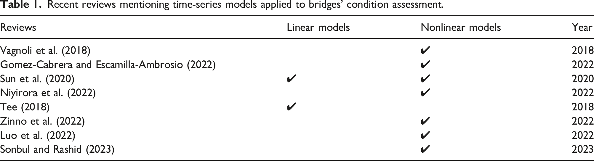
This table highlights the absence of recent comprehensive reviews focusing on the application of linear models to the field of bridge condition assessment. Among the limited number of reviews that use linear models, only one, Tee (2018), stands out for its thorough theoretical description; however, concerning the applications, the author does not analyze in deep the bridges structures. In contrast, while a considerable volume of reviews has examined nonlinear models, a significant portion of these predominantly concentrates on ANNs and CNNs. Additionally, almost none of them analyses the nonlinear together with linear models, elucidating its differences, potentialities, and limitations. Only Sun et al. (2020) briefly mention both linear and nonlinear models, and RNN and LSTM, yet offer only a brief introduction.

In turn, the specific application of these models to the domain of railway bridges is scarce in the existing literature. To address this gap, Figure 1 presents the process of a Scopus database search. This first search intends only to grant an overview about time-series model applied in damage detection on bridges. The keywords used are grouped into three specific categories: models, goals, and application. The search logic with the terms used in the query are presented with examples. Also, the filters used to select only the results related to bridges are condensed, and finally, the proportions of the outcomes that are related to railway or highway bridges.

Figure 1.

Scopus search process and results’.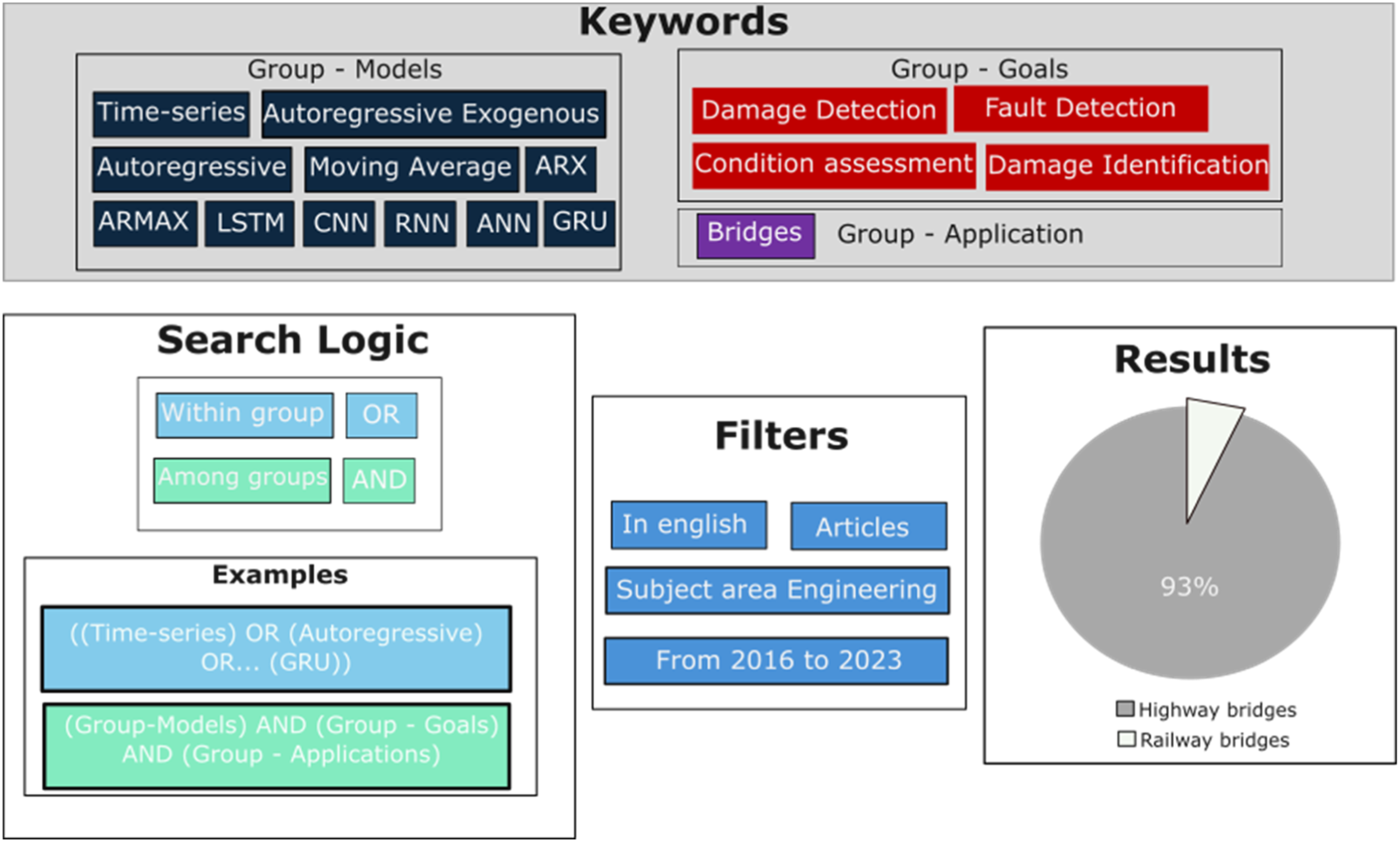

Figure 1 demonstrates a discernible disparity in research attention between railway bridges and highway bridges in the context of time-series models’ and SHM. Hence, there is a lack of comprehensive reviews covering both linear and nonlinear time-series models used in assessing bridge condition state. Therefore, this review intends to contribute addressing the following gaps:

• Absence of reviews considering simultaneously both linear and nonlinear time-series models in SHM context, discussing its architecture, inherent potentialities, and limitations.

• Limited quantity of reviews detailing and examining the applications of RNN, GRU, LSTM, and NARX models in the context of bridges’ condition assessment.

• Lack of reviews that comprehensively analyze time-series models specifically applied to the diagnosis of damage in railway bridges.

Addressing these topics, initially, an overview is conducted using relevant publications related to the application of time-series models to bridges. This section lays out the theoretical basis, explaining the linear models AR, ARMA, ARX, ARMAX, ARIMA, the nonlinear models ANN, CNN, RNN, NARX, GRU and LSTM, and their proper use, regarding real-world SHM applications. Next, only studies that applied the models to condition assessment in railway bridges are discussed. This section describes the efficiency of linear models when combined with normalization procedures in identifying damage and even assessing its severity or localization. Moreover, it outlines the ability of nonlinear models to address EOVs and explores the potential for damage localization through the implementation of exogenous inputs and severity assessment, mainly by hypothesis testing. Finally, the paper review is summarized, outlining the challenge associated with optimizing hyperparameters of time-series models, accounting for EOVs, and training the models to applications in real-world scenarios.

Overview of time-series models for condition assessment of bridges

Time-series models serve as an efficient methodology used in signal processing and feature extraction applications. For SHM, an initial model, corresponding to a reference condition, that is, without damage, is trained by fitting models’ coefficients to time-series data (acceleration, displacement, strains, etc.) with the primary aim of forecasting responses. Later, this process is repeated for data supposedly altered by damage. The coefficients and residuals of the obtained models (difference between the model prediction and the measured values) are expected to change (Entezami and Shariatmadar, 2019; Tee, 2018). For the coefficients, these changes may be identified upon recalibration of the model using a dataset featuring structural damage. For the residuals, changes in the statistical distribution might be noted (Entezami and Shariatmadar, 2019; Farahani and Penumadu, 2016; Tee, 2018).

The time-series data, used to build the models, can be classified into four distinct categories: (i) stationary or non-stationary; (ii) linear or nonlinear; (iii) univariate or multivariate; and (iv) Gaussian or non-Gaussian (Entezami, 2021; Kitagawa, 2010). Stationarity refers to the variability of statistical moments within a dataset. As depicted in Figure 2, where stationary (a) and non-stationary data (b and (c) with respect to the mean are illustrated. Additionally, Figure 2(d) shows data that is non-stationary with regards to variance.

Figure 2.

Sample signals illustrating time-series data: (a) stationary and linear (b) non-stationary and linear (c) non-stationary and non-linear (d) non-stationary and linear.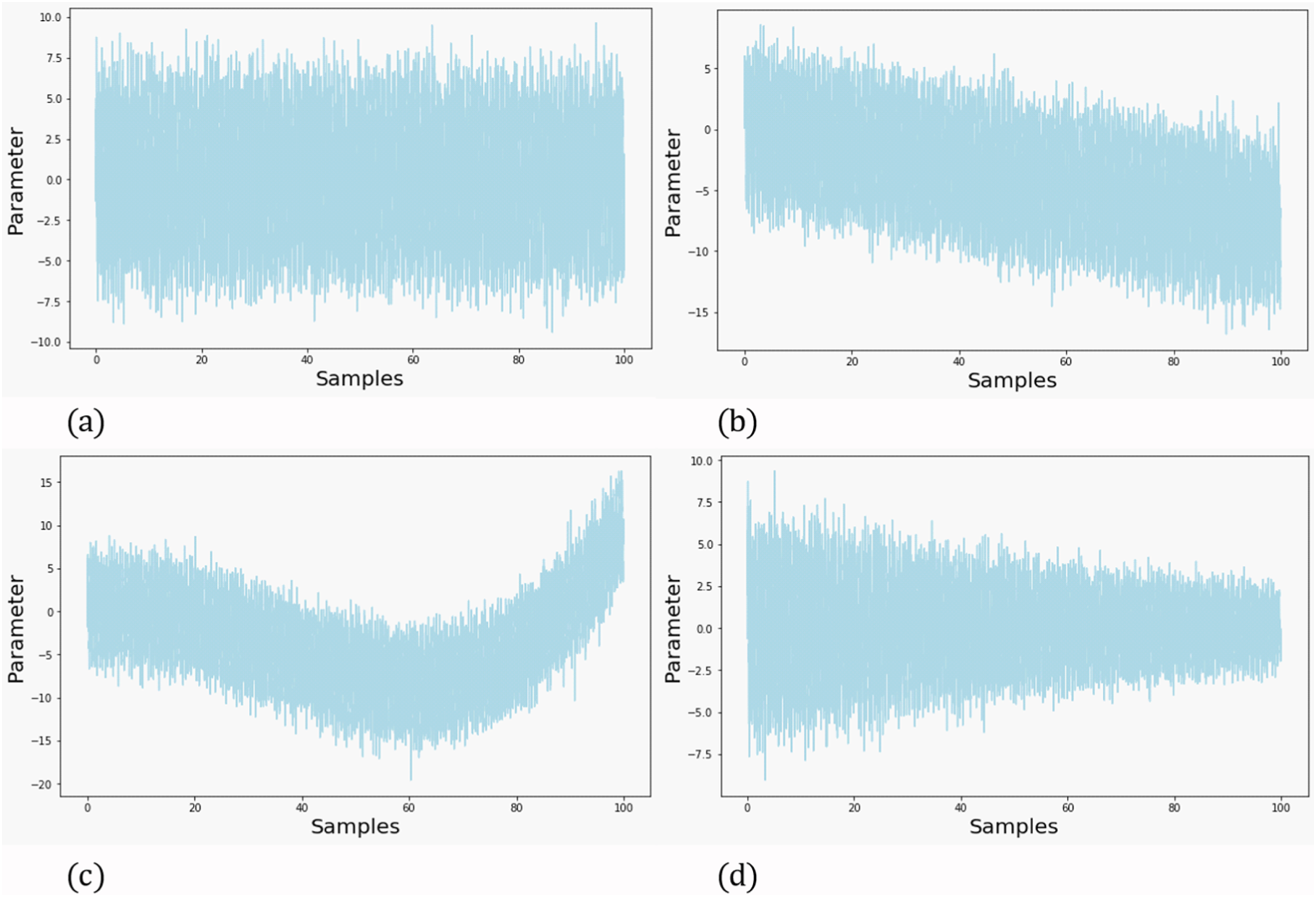

Furthermore, the categorization of linear and non-linear concerns the suitability of data to be reproduced. Figure 2(a)–(d) depict linear data, whereas Figure 2(c) illustrates nonlinear data. Moving forward, the distinction between univariate and multivariate data relate to whether it consists into single or multiple features. Since data is usually collected from multiple sensors, most time-series data are multivariate. However, the models can employ them individually or together. Lastly, classification into Gaussian or non-Gaussian depends on whether the distribution is normal or not. The categorization of a given dataset plays a crucial role in determining the most suitable time-series model, thereby improving the predictive performance.

For instance, when examining the pure acceleration response of a railway bridge, it tends to exhibit features of stationarity, linearity, and Gaussian distribution. This inherent stationarity allows time-invariant models, such as linear models, to effectively predict responses across a defined time window (Azim and Gül, 2020; Datteo et al., 2018; Matsuoka et al., 2021; Meixedo et al., 2022). However, as there are environmental and operational variations (EOVs), normalization must be done, especially to the aforementioned models, due to the presence of nonlinear responses (Azim, 2021; Meixedo et al., 2022; Wang et al., 2022). Furthermore, the Gaussian nature of the data allows for efficient anomaly detection through hypothesis testing, established with a designated confidence boundary (Meixedo et al., 2021; Santos et al., 2016). On the other hand, nonlinear models demonstrate versatility across a wide spectrum of time-series data (Chalouhi et al., 2017; Lawal et al., 2023; Wang et al., 2022). Essentially, they could capture complex nonlinear relationships as well as perform data compression and fusion operations.

In the context of the railway bridges damage diagnosis, this paper will focus on the description of both linear models and nonlinear time-series models. Figure 3 highlights the chosen models within these paradigms, which will undergo comprehensive analysis. The linear time-series models section will provide a brief overview of the widely employed linear models in the context of SHM. Subsequently, The nonlinear time-series models section will elaborate on nonlinear time-series models, including methods that consider sequential data structures such as RNN, NARX, GRU, and LSTM, as well as those that do not, necessarily, rely on it, such as ANN and CNN.

Figure 3.

Analyzed time-series models.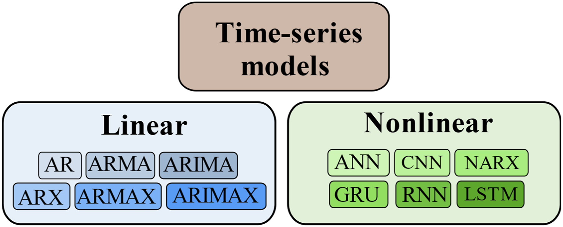

Linear time-series models

Fundamental autoregressive models assume that the outputs of a specific time-series data exhibit a linear dependence on their preceding values, along with a stochastic element. This concept is summarized in equation (1), which defines the AR model:

y (t) = \sum_{i = 1}^{n_{a}} ϕ_{i} y_{t - i} + ε (t)

(1)

Where

n_{a}

is the model order,

y_{t}

are the system responses,

ϕ_{i}

are the coefficients or parameters, and

ε (t)

is the error term, or white noise, of the model. Usually, a least square minimization is used to determine

ϕ_{i},

and

ε (t)

is the difference between the measured and the predicted response. Datteo et al. (2018) discuss the application of AR models for characterizing simple dynamic systems under stochastic excitation and their use for damage classification. They explore an enhanced framework for damage detection using various types of datasets, highlighting the limitations inherent to these models.

In scenarios where responses are observed across multiple points (a multivariate time-series), the response at each sensor can be forecasted using the output from a chosen reference channel together with inputs from other channels. This methodology is the exogenous autoregressive model (ARX), as represented in equation (2):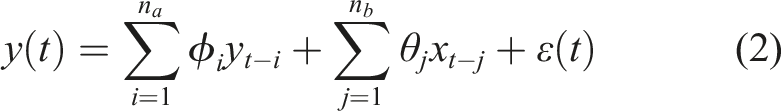

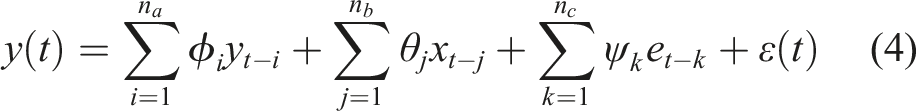
y (t) = \sum_{i = 1}^{n_{a}} ϕ_{i} y_{t - i} + \sum_{j = 1}^{n_{b}} θ_{j} x_{t - j} + ε (t)

(2)

Where

n_{b}

is the model order and

θ_{j}

the model coefficients for the inputs. Proper clustering must be done to only use sensors that retain relevant information (Farahani and Penumadu, 2016). Even though ARX models are more capable of describing systems in the SHM context, environmental and operational variations (EOVs) affect the responses (Azim, 2021; Meixedo et al., 2022; Wang et al., 2022), and subsequently, the error term for both AR and ARX models. Hence, models that consider functions to describe

ε

are less prone to EOV perturbations (Parisi et al., 2022).

One possible way is to introduce an error equation, usually associated with Moving Average processes (MA) (Sonbul and Rashid, 2023), in AR (equation (1)) or in ARX models, obtaining, respectively, the autoregressive moving average (ARMA), described by equation (3), and the moving average exogenous autoregressive models (ARMAX), expressed in equation (4).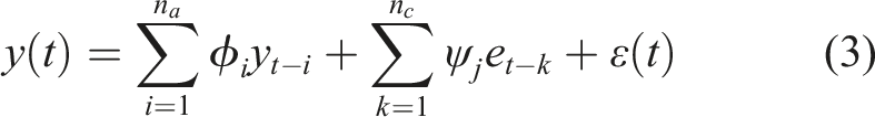

y (t) = \sum_{i = 1}^{n_{a}} ϕ_{i} y_{t - i} + \sum_{k = 1}^{n_{c}} ψ_{j} e_{t - k} + ε (t)

(3)

y (t) = \sum_{i = 1}^{n_{a}} ϕ_{i} y_{t - i} + \sum_{j = 1}^{n_{b}} θ_{j} x_{t - j} + \sum_{k = 1}^{n_{c}} ψ_{k} e_{t - k} + ε (t)

(4)

Where

n_{c}

is the order and

ψ_{j}

are the coefficients for the error. The main advantage of ARMA and ARMAX models is that they filter the noise from various sources in the measurements, providing unbiased parameter estimates (Hu et al., 2015; Lakshmi & Rama Mohan Rao, 2016).

The previous models are based on the stationarity of data. When there is no stationarity on the raw data, the difference between the responses, may be considered in the time-series model. The Autoregressive Integrated Moving Average (ARIMA) and its version with exogenous input (ARIMAX) models use this approach, subtracting the current value from a previous value. To a simpler representation of the model, the backshift operator $B$ is introduced, representing the action of shifting the sequence one time step into the past. $B^{k}$ applies this action to shift the sequence k time steps backward as represented in equation (5).

B^{k} y_{t} = y_{t - k}

(5)

The difference between measures is defined by equation (6).

\nabla y_{t} = y_{t} - y_{t - 1}

(6)

Dividing both sides by $y_{t}$ the difference operator ( $\nabla)$ is defined. Then the ARIMA and ARIMAX models, of order $n_{d}$ are defined, respectively, by:

Φ (B) \nabla^{n_{d}} y_{t} + ε (t) = Ψ (B) e_{t}

(7)

Φ (B) \nabla^{n_{d}} y_{t} + ε (t) = Ψ (B) e_{t} + Θ (B) x_{t}

(8)

Where:

Φ (B) = 1 - \sum_{i = 1}^{n_{a}} ϕ_{i} B^{i}

(9)

Θ (B) = 1 - \sum_{j = 1}^{n_{b}} θ_{j} B^{j}

(10)

Ψ (B) = 1 - \sum_{k = 1}^{n_{c}} ψ_{j} B^{k}

(11)

The model order $n_{d}$ indicates the number of times the subtractions operations are done to achieve stationarity. Based on the ARIMAX model, the other models can be obtained when considering $n_{b}$ , $n_{c}$ or $n_{d}$ as zero. For instance, for $n_{d} = 0$ the ARMA model is obtained, for $n_{d} = 0$ and $n_{c} = 0$ , ARX model is obtained. Illustrating this relation among the models, Figure 4 summarizes the key structural aspects them.

Figure 4.

Autoregressive models’ structure.

Finally, the estimation of the model order is of utmost importance for accurately capturing temporal patterns. For linear endogenous models, the use of criteria such as the Bayesian Information Criterion (BIC) or Akaike Information Criterion (AIC) is common (Datteo et al., 2018; Meixedo et al., 2022). For exogenous or non-linear models, criteria such as Mean Squared Error (MSE), Normalized Root Mean Square Error (NRMSE), Mean Absolute Error (MAE), among others, have proven to be suitable for order selection (Gong et al., 2023; Meixedo et al., 2021; Tee, 2018; Wang et al., 2022).

Nonlinear times-series models

Given that the connections between attributes that perturb an analyzed response often arise from nonlinear combinations, the development of a framework capable of accurate prediction requires the integration of nonlinear models. For SHM, a particularly suitable method is the use of ANNs, which will be briefly discussed below.

The ANN is an efficient nonlinear statistical model well-suited for both classification and regression tasks. At its core, this model comprises processing elements, or neurons, that employ nonlinear functions to map attributes to corresponding outputs (Finotti et al., 2019). The topology of an ANN is commonly represented through a network diagram, as depicted in Figure 5.

Figure 5.

ANN network diagram.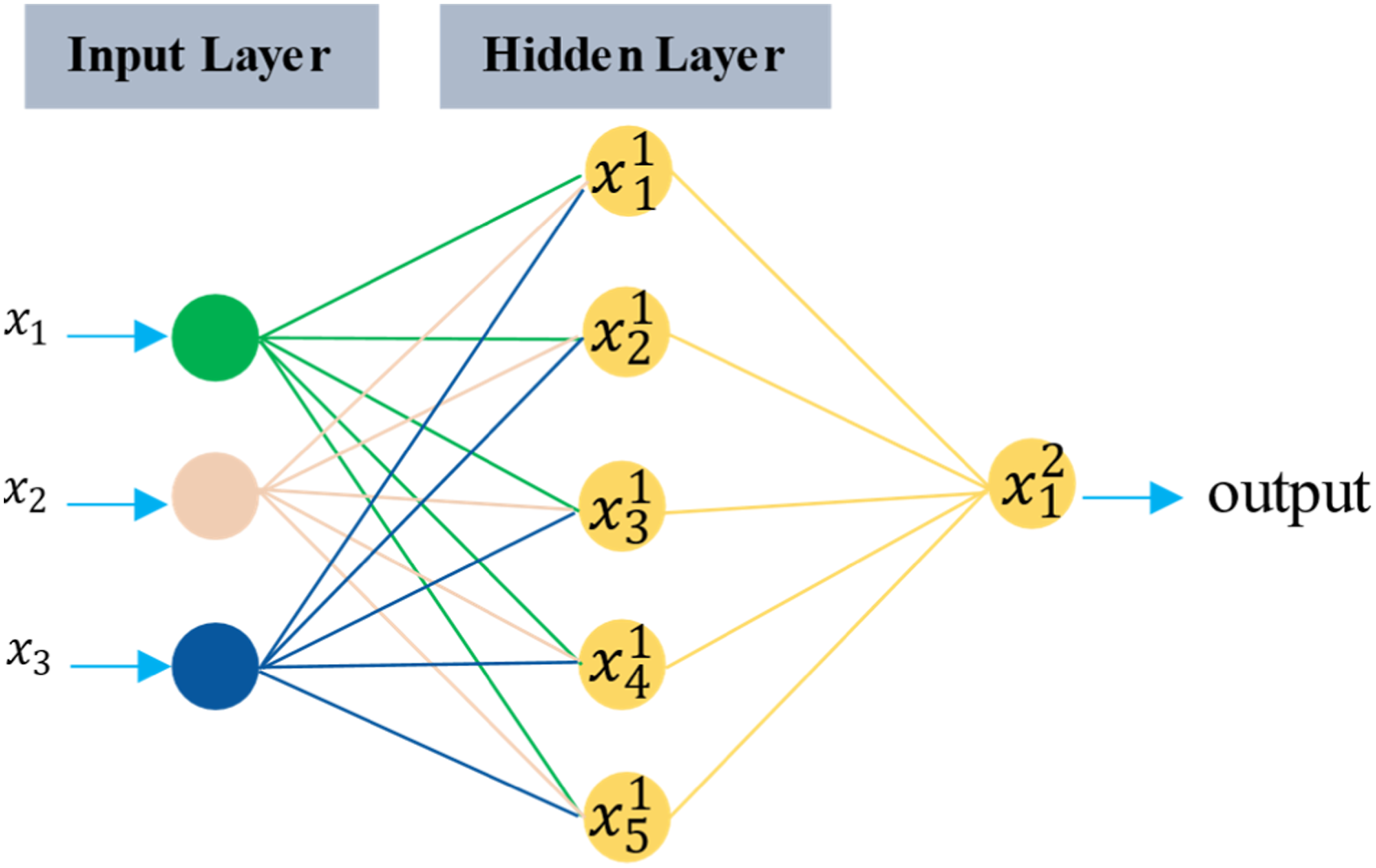

Where $x_{1}$ , $x_{2}$ , and $x_{3}$ are the inputs or attributes, the intermediary nodes (yellow) are designated hidden layer and $x_{1}^{2}$ is the output. Each arrow represents a weight ( $W)$ , and each node on the next layer is a transformation of the attributes in the last one. For Figure 5, each node in the hidden layer ( $h$ ), may be written in matrix notation as equation (12).

h = σ (W_{h}^{T} x + b_{h})

(12)

Where

σ

represents the activation function designated by the user and

b_{h}

signifies the bias of the hidden layer. The configuration of the ANN encompasses the flexibility to modify the number of inputs, intermediary layers, nodes per layer, and even outputs. Furthermore, the option exists to employ several activation functions for different layers (Vagnoli et al., 2018; Gomez-Cabrera and Escamilla-Ambrosio, 2022). The coefficients

W

are determined by minimizing an objective function, often referred as loss function. It is important to note that when

σ

is selected as the identity function, that is,

σ (x) = x

, the ANN simplifies into a linear model based on the inputs. Therefore, an ANN can be comprehended as a nonlinear extension of linear regression and classification models (Lim and Zohren, 2021). Over time, ANN models went through gradual adaptations to deal with specific goals, including the more efficient handling of big data. A notable example is the CNN, depicted in Figure 6, which leverages convolution operations in its layers to extract complex features from the input data. This is subsequently followed by pooling layers that facilitate the extraction of dominant features while concurrently reducing dimensionality.

Figure 6.

Basic CNN architecture.

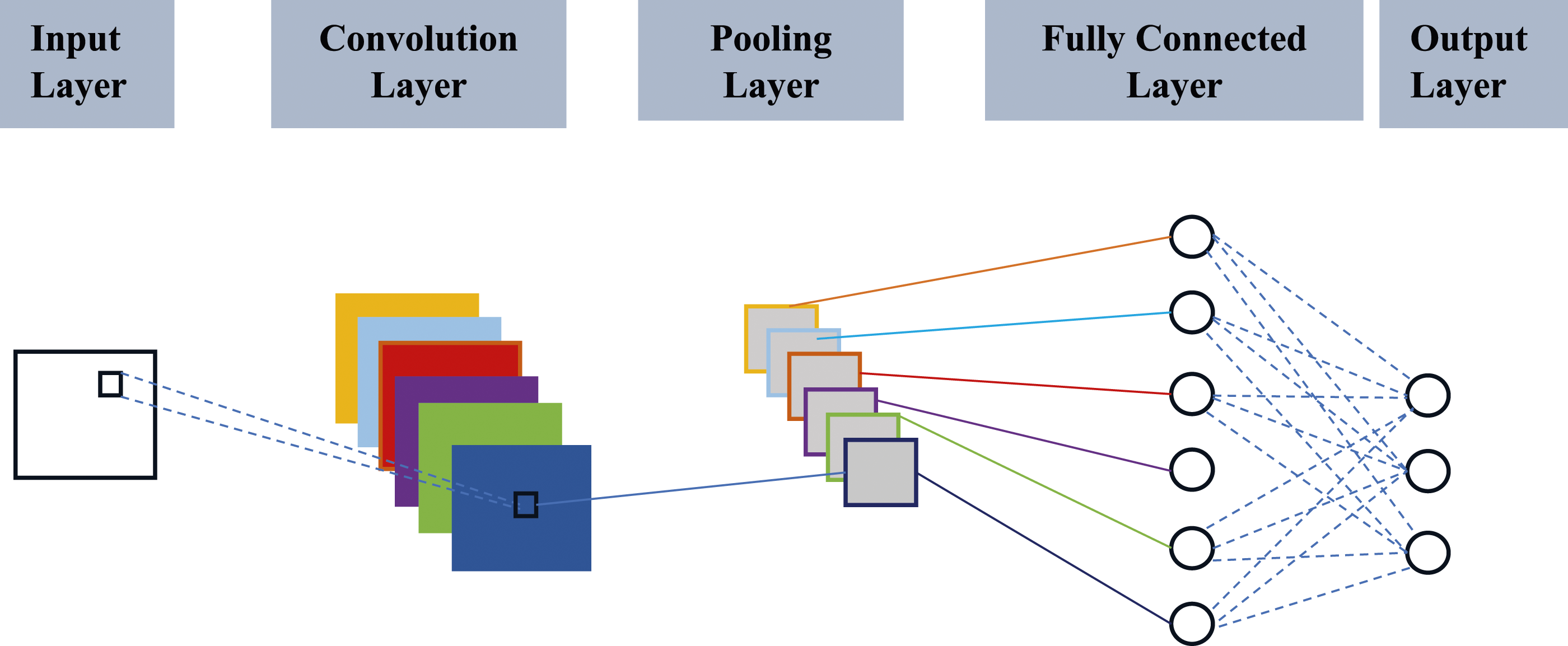
Lastly, the outcomes derived from the pooling layers are integrated as inputs into an ANN. A typical CNN architecture encompasses a sequence of operations, namely feature extraction, normalization, and data compression. Despite the prevalent association of CNNs with image processing, their use extends beyond that, including applications within SHM. Even multivariate time-series data can profit from the inherent capabilities of this model (Parisi et al., 2022).

Regarding sequential data, RNN, NARX, GRU, and LSTM stand as more efficient propositions for ANN models. RNN employs node (neuron) outputs as feedback to nodes in previous layers, like a NARX definition. The distinction lies in NARX’s integration of exogenous inputs. Figure 7 showcases a rudimentary unfolded RNN architecture.

Figure 7.

Unfolded RNN architecture.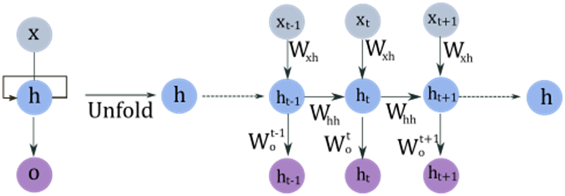

To the RNN exemplified in Figure 6 the values on the hidden layers are recursively calculated by equation (13):

h_{t} = σ (W_{x h}^{T} x_{t} + W_{h h}^{T} h_{t - 1} + b_{h})

(13)

And the output is calculated by equation (14):

{\hat{y}}_{t} = σ (W_{o}^{t} h_{t} + b_{o})

(14)

Where

W

are the weights,

x_{t}

are attributes values at time

t

h

are the hidden nodes values, and

b

the layer bias. The first and the last subscripts refer to original and final layer respectively. Subscripts

x

refers to the inputs,

h

to the hidden layers and

o

to the outputs. The weights are updated according to the relative gradient, which is calculated recursively from the output layer towards the input layer.

For the NARX model depicted in Figure 8, each response function is a product of endogenous ( $x_{t}$ ) and exogenous inputs $(y_{t - n_{y}})$ . Additionally, $h_{t}$ is the hidden layer values, $W_{1}$ and $W_{2}$ represent the weights to the first and second layer, respectively. In this context, a specific sensor response acts as the reference (endogenous input), while neighbor sensors serve as exogenous inputs, thus an adequate sensor cluster is essential (Umar et al., 2021).

Figure 8.

NARX model with 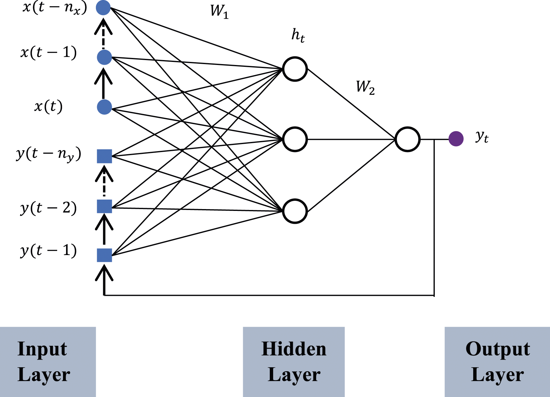$n_{x}$ inputs and $n_{y}$ outputs.

The incorporation of these supplementary inputs involves the inclusion of an additional term in equation (14). As a result, the model is given by:

y_{t} = σ (z (t)) + e (t) = σ (x (t), \dots, x (t - n_{x}), y (t - 1), \dots, y (t - n_{y})) + e (t)

(15)

Where

z (t)

is the regression vector of current and past values,

n_{x}

and

n_{y}

are the maximum input and output lags, equivalent to number of input and outputs used to forecast the next value. The error function is assumed to have a standard normal distribution, which is reasonable considering the central limit theorem (Entezami, 2021). This is aligned with recent studies showing that the NARX model prediction error is a DSF capable of giving damage location and severity information based on this assumption (Umar et al., 2021; Yan et al., 2013).

The RNN may be obtained from the NARX by using solely the output values. In turn, the RNN is a nonlinear generalization of a linear regression applied to sequential data, such as time-series data. In particular, the prediction of RNNs relies on the second derivatives within each hidden layer. However, this architectural design can be susceptible to the vanishing gradient problem, that is, the situation where the gradients of the loss function with respect to the model’s parameters become extremely small as they are backpropagated through multiple layers during the optimization process. Therefore, the algorithm exhibits problems in learning from inputs distanced from the predicted response. For instance, in the work by Bui-Ngoc et al. (2022), a CNN-RNN framework was applied to acceleration measurements using the well-known Z-24 bridge benchmark. Despite employing CNN for data compression, the loss function for training and test dataset did not converge (due to overfitting) which might lead to inadequate results to real world application.

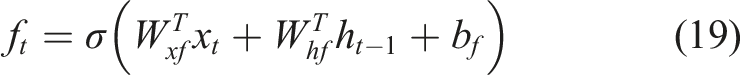
One effective strategy to tackle this issue involves incorporating neurons, or gates, that explicitly facilitate the retention or omission of inputs. This innovative model is termed GRU, and its mathematical representation is illustrated in equation (16):

h_{t} = (1 - z_{t}) ⊚ h_{t - 1} + z_{t} ⊚ \tanh ({W_{x h}}^{T} x_{t} + {W_{h h}}^{T} (r_{t} ⊚ h_{t - 1}) + b_{h})

(16)

Where

z_{t}

and

r_{t}

are, respectively, the update gate vector and the reset gate vector, given by:

z_{t} = σ ({W_{x z}}^{T} x_{t} + {W_{h z}}^{T} h_{t - 1} + b_{z})

(17)

r_{t} = σ (W_{x r}^{T} x_{t} + W_{h r}^{T} h_{t - 1} + b_{r})

(18)

The subscripts indicate the layer of the weights and biases, and $⊚$ is the element wise multiplication (element per element) symbol. Both $z_{t}$ and $r_{t}$ are logical units that may be interpreted as a logistic regression with outputs ranging from 0 to 1. Thus, when $z_{t}$ is closer to 1, the previous value is less considered by the model. The reset gate vector is just another gate to grant further capacity to the model to retain or discard inputs from the previous layers.

In recent applications of GRU within the context of SHM, some employ the model in conjunction with a CNN framework. In this setup, CNN serves to model spatial relationships and short-term temporal connections among various sensors in an instrumented bridge. The output of the CNN is then input to a GRU, enabling the learning of long-term temporal dependencies. Notably, these combined models have demonstrated remarkable accuracies, achieving 94.92% for a laboratory-scaled concrete bridge and 85.11% for a three-story frame structure from the well-known IASC-ASCE Benchmark (Yang et al., 2020, 2021).

The concept of LSTM was initially introduced to address the vanishing gradient problem inherent in RNNs. In historical context, the GRU can be regarded as a simplification of the LSTM architecture. The equations utilized for the LSTM model are as follows:

f_{t} = σ (W_{x f}^{T} x_{t} + W_{h f}^{T} h_{t - 1} + b_{f})

(19)

i_{t} = σ (W_{x i}^{T} x_{t} + W_{h i}^{T} h_{t - 1} + b_{i})

(20)

o_{t} = σ (W_{x o}^{T} x_{t} + W_{h o}^{T} h_{t - 1} + b_{o})

(21)

c_{t} = f_{t} ⊚ c_{t - 1} + i_{t} ⊚ f_{c} (W_{x c}^{T} x_{t} + {W_{h c}}^{T} h_{t - 1} + b_{c})

(22)

h_{t} = o_{t} ⊚ f_{h} (c_{t})

(23)

Where

f_{t}

i_{t}

, and

o_{t}

are forget, input and output gates, respectively;

c_{t}

and

h_{t}

are the cell state and the hidden state;

f_{c}

and

f_{h}

are the activation function for the cell and hidden state. Once again, each gate may be seen as a neuron, varying from 0 to 1 regulating how much of information will be retained. The cell state

c_{t}

is the weighted sum of the previous cell state by the simple RNN (in the parenthesis of equation (15)) weighted by the forget and input gates. Sharma and Sen (2023), illustrate the efficiency of LSTM detecting damage in a highway bridge even with 1% stiffness loss with accuracy above 90% for different simulated noises scenarios, without any prior EOV filtering process. Finally, Table 2 summarizes key features of the models. By being nonlinear, they are all able to handle EOV more efficiently.

Table 2.

Models’ features.

Nonlinear model	Exogenous inputs	Recursive structures	Logical gates	Data fusion	Data compression
ANN
CNN	✓			✓	✓
NARX	✓	✓		✓
RNN		✓
GRU		✓	✓		✓
LSTM		✓	✓		✓

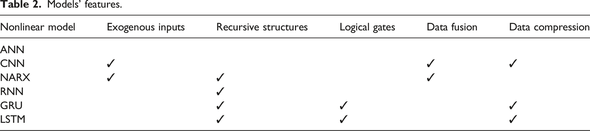
From the information presented in Table 2, it becomes evident that the ANN model, in comparison, assumes the role of a fundamental nonlinear model. Furthermore, the architectures of the GRU and LSTM models share similarities. The primary distinction resides in the quantity of logical gates, which facilitates more effective data regulation during the training process. Notably, the “Data Compression” column pertains to models featuring distinctive structures, like pooling layers in CNN or the forget gates within GRU and LSTM architectures.

Application of time-series models for condition assessment of railway bridges

Linear time-series models

The selection of each study to be analyzed in this section, was grounded in their relevance to the chosen focus, that is, works that utilized time series models for damage identification in railway bridges. This selection was based on theoretical consistency and coherence, author metrics such as the number of citations and h-index, as well as the metrics of the works themselves. Consequently, only publications that are relevant, recognized by the academic community, indexed in reliable databases, and that bring relevant aspects in the use of time-series models were selected.

Linear models offer a range of applications owing to their adaptability, efficiency, and economical computational requirements. These attributes manifest across diverse datasets (Azim, 2021; Datteo et al., 2018; Meixedo et al., 2022) and performance (Azim and Gül, 2020; Meixedo et al., 2021) on the methodologies outlined in overview of time-series models.

Azim and Gül (2019) introduced an enhanced damage strategy rooted in the ARX framework (equation (2)), building upon a similar methodology proposed by Mei and Gül (2016). In the updated version, biaxial acceleration responses and operational variables (train speed and loadings) were incorporated. A Finite Element Model (FEM) encompassing the deck, girders, and track was developed to simulate baseline and impaired responses. The model consisted into five beam elements for the girders and a plate element for the steel deck supporting one single track with no description of its modelling. The supports were considered as hinges, restraining only translation. The train was COOPER E80 with the corresponding loading schema defined according to the American Railway Engineering and Maintenance of Way Association. Four distinct damage scenarios were replicated: stiffness reduction in beams, loss of moment capacity, alterations in support restraints, and deck stiffness deterioration. The selected DSF was the fitting ratio (FR), defined as follows:

F R = (1 - \frac{∥ y_{m} - y_{s} ∥}{∥ y_{m} - μ ∥})

(24)

Where

y_{m}

is the measured output,

y_{s}

is the predicted output and

μ

is the mean of the measured output. Since

F R

is different as the exogenous input is changed, the difference between two measured features normalized by a reference response, or Damage Feature (DF), given by:

D F = \frac{| F R_{1} - F R_{2} |}{F R_{1}} \times 100 %

(25)

This feature allows damage severity and location assessment, even though always in reference to a fixed benchmark. In essence, this feature is a distance-based metric for anomaly detection, as the difference between a reference state and a damaged is expected to increase as abnormality becomes greater. Furthermore, the feature is expected to increase when close to a localized damage. Consequently, the strategic deployment of the sensor network assumes a crucial role in determining the effectiveness of location-related data. The endogenous and exogenous order of the model was determined solely based on physical modeling and subsequently fixed, whereas the more appropriate procedure for establishing it should rely on metrics such as the Akaike Information Criterion (AIC), Bayesian Information Criterion (BIC), Normalized Root Mean Square Error (NRMSE), among others (Datteo et al., 2018). Without such metrics is not possible to understand if the chosen model order correctly captured the system dynamics.

While the threshold was established based on the outcomes of baseline simulations, the statistical methodology for achieving the specified 99.7% confidence level was solely based on the DFs obtained to the reference state. Some outcomes are presented in Figure 9.

Figure 9.

DFs to beams N1 to N10 with stiffness loss of: (a) 10% (b) 40% (Azim and Gül, 2019).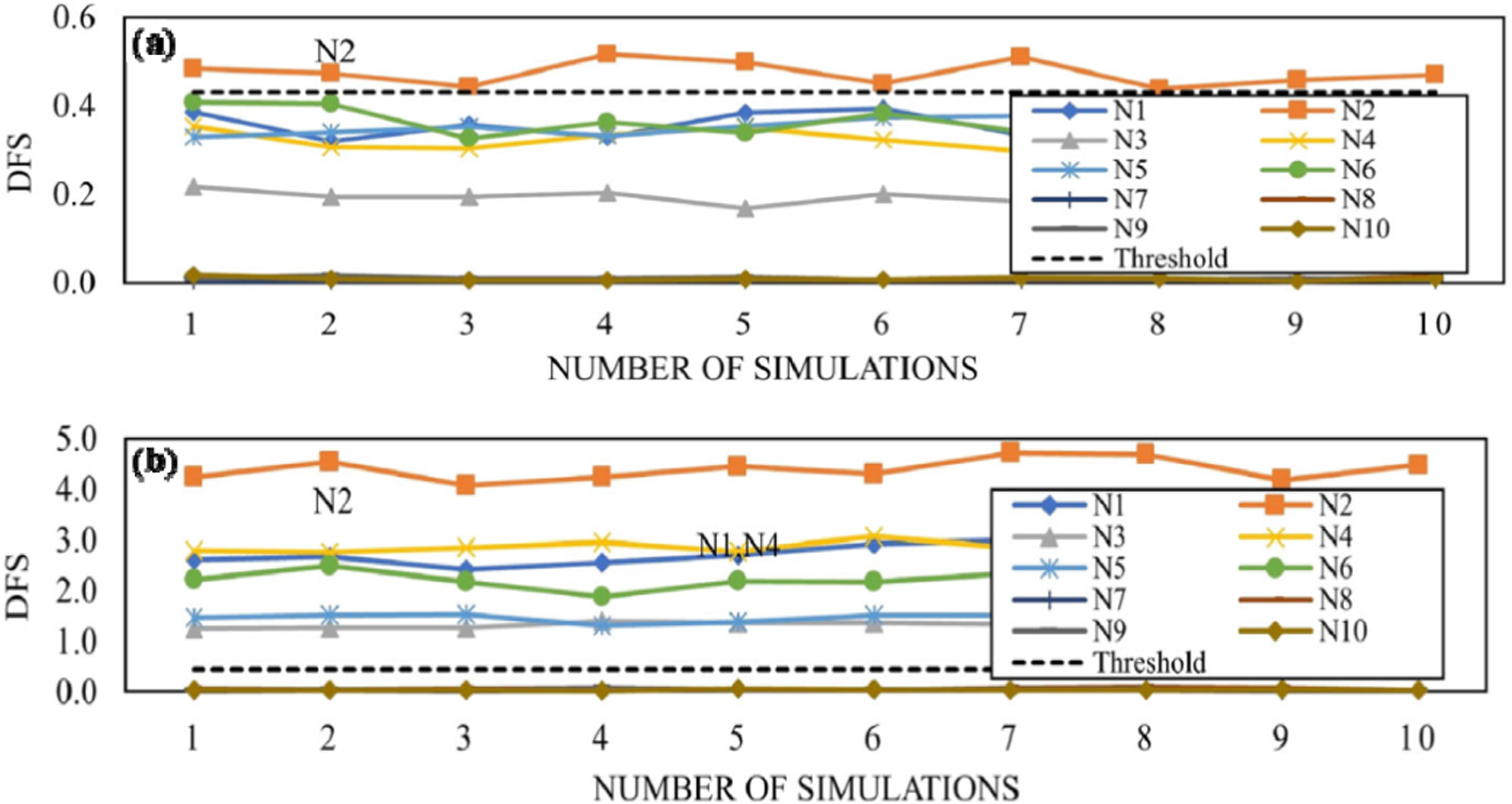

The outcomes showcased the model’s ability to gauge severity of a specific damage, as higher DFs values corresponded to more pronounced modeled damages. Furthermore, for beams with simulated damage (beam N2), higher DFS values were obtained for nodes of the damaged bars. This sensitivity to damage location is particularly pronounced for larger reductions in stiffness.

The study illustrates the damage sensitivity of the indicator for the specific scenario proposed. However, the approach could benefit from employing statistical discrimination methods, such as distances or statistical distributions, coupled with thresholds and subsequent associated metrics, to facilitate a more detailed analysis of the methodology’s performance.

A comparable study undertaken by the same research group (Azim and Gül, 2020) followed a similar trajectory with slight adjustments in the confidence level (99%). This methodology was applied to a distinct railway truss bridge model featuring alternative damage scenarios. The authors crafted a FEM to generate reference acceleration responses (unchanged or baseline) and damage configurations involving 20%–30% stiffness loss in specific bars. Clusters were made to train an ARMAX models using only the neighbor’s sensors information, without explicitly explain the criteria for that selection.

Notably, the proposed DSF could detect damage location and severity as increasing stiffnesses losses resulted in increasing DF only to the damaged bars. While the proposed damage detection framework demonstrates proficiency in offering damage localization insight, to the specific tailored example, its applicability to experimental data and strategies addressing EOV remains unexplored. This could potentially represent a limitation of the method, given that the employed autoregressive models are fundamentally linear in nature. Furthermore, this study also has the same issues of the previous concerning model order, statistical discrimination strategies and absence of metrics that could allow to better analyze the framework performance.

Conversely, Meixedo et al. (2021) used the potential of linear models in a robust damage detection methodology. Initially, the authors conducted the modeling and validation of the finite element model of the bridge over the Sado River, utilizing real data (Meixedo et al., 2022). The model was meticulously constructed, considering various components such as piers, sleepers, ballast-containing beams, rails, arches, hangers, transverse stiffeners, diaphragms, and diagonals as beam elements, as well as the concrete slab and the steel box girder as shell elements, among other elements. The support was modeled considering the bearing devices at the top of each pier. The validation of the static behavior of the model was conducted using temperature data. Meanwhile, the validation of the dynamic behavior was performed by simulating the passage of an Alfa Pendular train traveling at 216 km/h.

The authors introduced AR coefficients that underwent normalization through two distinct techniques: Multiple Linear Regression (MLR) and Principal Component Analysis (PCA). In the MLR-based normalization, temperature and train speed were used as inputs to a multivariate linear regression model, with AR coefficients serving as outputs. Next, the responses obtained using these coefficients were used to subtract the EOVs effects from the acceleration records.

The second normalization type, based on PCA, involved an orthonormal projection into a lower-dimensional vectorial subspace. By progressively discarding principal components associated with higher retained variance, the method aimed to filter out EOVs (Rastin et al., 2021). This sequential reduction in dimensionality helped to mitigate their impact on the analysis.

Subsequently, the Mahalanobis Distance (MD) was employed to fusion data from distinct sensors, condensing information about a given state into a single index that aimed to gauge the dissimilarity between responses. Generally, the distance-based methods presume that outliers will have significantly different distances from the normal behavior. In this study, the MD for the damage scenarios dataset is expected to increase from the reference scenarios.

The index obtained by calculating MD was not flagged based on supervised judgment. A Confidence Boundary (CB) was defined through the application of an inverse cumulative distribution function (ICDF), clustering MD outputs into damage or undamaged states, in a more objective and robust approach. The framework addressed AR model limitations regarding EOV, while using their potential. The model’s adequate performance was underscored by the framework’s application to data simulated via a well calibrated model of the Sado River railway bridge. Following the validation of a FEM through monitoring data, as previously mentioned, multiple damage scenarios were simulated and the noise, which was measured on site, was added to each corresponding sensor. The damage scenarios were simulated based on the most feasible occurrences due to bridge’s vulnerabilities. Those related to corrosion and friction increments in the bearing devices were assumed as most likely.

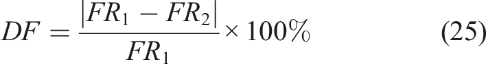
Acceleration responses from 100 simulations, accounting for varying temperature, train models, and speeds, were leveraged to establish the reference baseline state. An additional 114 simulations were conducted to simulate damage scenarios involving stiffness reduction in bridge elements and an increase in friction coefficients at bearings, with varying degrees of severity. The primary outcomes are depicted in Figure 10.

Figure 10.

DI to four damaged scenarios varying environmental and operational conditions with CB to: (a) MLR-based features (b) PCA-based features (Meixedo et al., 2021).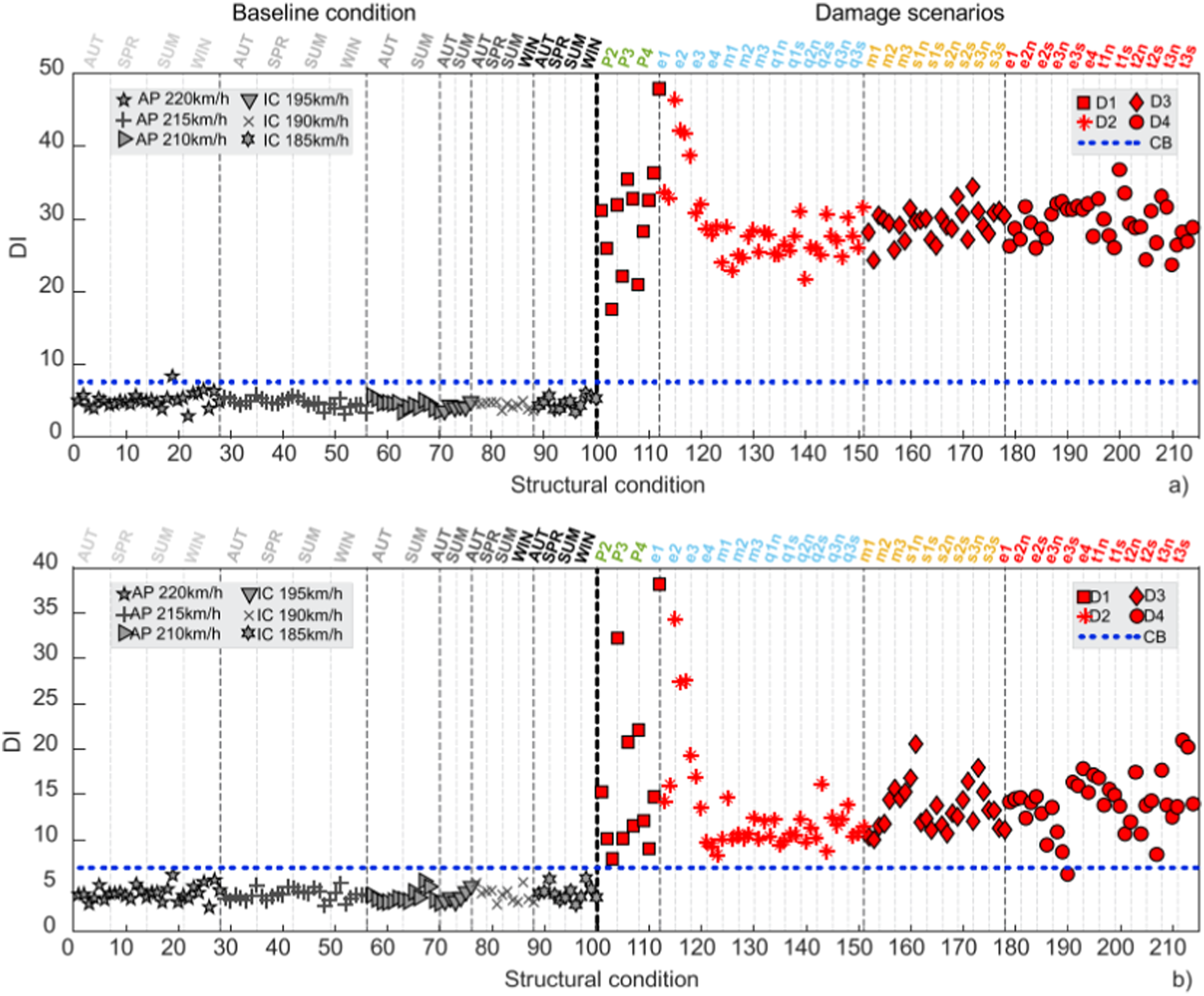

Figure 10 provides a visual representation of the sensitivity and stability of the Damage Index (DI) concerning various simulated EOV conditions. The MLR-based framework demonstrated a mere 1% Type-I error (False positive), while the PCA-based framework exhibited a 0.88% Type-II error.

The results present a consistent approach, estimating the endogenous order of the AR model using the BIC and employing distances associated with the ICDF, which reduces subjectivity in anomaly detection. However, the strategy employed does not facilitate the acquisition of metrics such as Cohen’s Kappa, F1-score, and F2-score, which are crucial for assessing the robustness of the method and its generalization capability (Grandini et al., 2020).

Given that AR coefficients constitute a univariate time-series model, they usually only identify damage. However, enhanced real-world applications may be achieved through exogenous models, like ARX or ARMAX. They leverage data from other sensors to achieve more accurate response modeling, particularly with respect to EOV and localization information, as presented in overview section.

In a recent advancement, the same authors exploited ARX as a feature extractor within an online and unsupervised damage detection framework (Meixedo et al., 2022). Apart from introducing cluster analysis for feature discrimination, the methodology closely reproduces the preceding steps—baseline and damage scenario simulations, feature extraction, normalization, and data fusion. On this approach, the ARX model order to a sensor, was chosen by minimizing NRMSE. One possible improvement would be to allow the model order of different sensors to vary within a cluster. Considering that the sensors are distributed spatially, the time-series data pattern are expected to change within a cluster. However, this implementation would increase the computational cost. Leveraging the k-means algorithm, this adaptation culminated in a fully automated, real-time damage detection framework.

The average dissimilarity between clusters (DC) is tested within a designated window of train passages, allowing the classification of bridge condition. After detailed assessment of optimal window length and the influence of the number of sensors, the outcomes surpassed those of the AR model. Remarkably, this framework effectively evaluated damage across diverse elements while maintaining a low false detection rate, as demonstrated in Figure 11.

Figure 11.

False detection rate to four different damage scenarios with varying window length (Meixedo et al., 2022).

Figure 11 depicts the efficiency of the online unsupervised methodology, identifying damages based on a moving window procedure comprising 19 train passages, keeping errors to a minimum. The proposed framework lacks the ability to localize damage, an aspect highlighted by the authors, who suggested considering extended applications of exogenous models as a potential way to achieve this goal. Nevertheless, the previous limitation regarding the metrics used for performance evaluation persists. The isolated assessment of the false detection rate does not permit generalizations, thereby not asserting that the methodology would be effective if applied in different scenarios.

Azim (2021) adopted a methodology comparable to their prior works (Azim, 2021; Azim and Gül, 2019), applied to the same bridge truss bridge (Azim, 2021) and using an equivalent DSF. The authors developed a simplified Finite Element Model (FEM) composed of bar elements. The supports at one end of the bridge were modeled as hinges, and at the other end, the pier supports were treated as rollers. Additionally, frictional resistance was not taken into account. The threshold encompassed incorporating two train types (E80 and E90) at speeds of 40 and 50 km/h and introducing artificial noise equivalent to 5% of the maximum Root Mean Square Error (RMSE). After executing 200 simulations, the threshold was set at 99%.

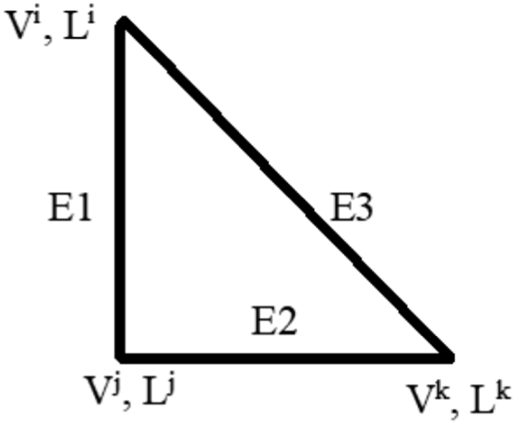
An additional modification entailed implementing PCA for strain measurements. Initially, the authors aggregated each sensor’s response into a matrix, subsequently applying PCA. The first two principal components, representing the most significant variances, were plotted onto a 2D plane using the eigenvectors of the strain matrix as axes. The distance between these components was then computed using the following equation:

D^{i} = \sqrt{{(Ψ_{1}^{i})}^{2} + {(Ψ_{2}^{i})}^{2}}, i = 1, 2, \dots, N_{s}

(26)

Where

Ψ_{1}^{i}

is the ith component of the first vector and

N_{s}

the number of sensors. Next the DFs obtained were normalized by its maximum value. Since on this methodology the DFs greaten than zero represents damage, all the DFs below zero were set to zero. Hence, the indicator is a distance-based feature for anomaly detection that does not need additional operation for classification. One more valuable contribution consisted in the element level analysis proposed which consists of a directional distance that allows a refined analysis for truss structures. To illustrate the process, consider the three truss elements in the Figure 12:

Figure 12.

Truss elements and nodes (Azim and Gül, 2021).

Consider the vertical monitored components $V_{i}$ , $V_{j}$ , $V_{k}$ , alongside the longitudinal components $L_{i}$ , $L_{j}$ , and $L_{k}$ , all obtained at distinct nodes. Consequently, the acquired DFs match to the response of a particular node. To extend these associated indices to an element level, the authors have introduced a method involving the multiplication of obtained values across both ends of an element. For instance, when solely element E1 is compromised, the multiplication of nodes E2 and E3 results in zero. This procedure effectively allows the accurate assignment of the damaged elements. Ultimately, to derive a Damage Feature specific to a given element ( $D F E_{s}$ ) from strain data, the applied DF is calculated as follows:

D F_{A + S} = D F E_{s} * (D F E_{V}^{″} + D F E_{L}^{″})

(27)

Where

D F E_{L}

is the damage feature used to detect damage into longitudinal and diagonal members,

D F E_{V}

to vertical and diagonal elements. Thus, when an index that identifies damage regardless of its location is weighted by the oriented indexes, the result (

{D F}_{A + S}

) removes false identifications, granting robustness to the methodology. Some of the key-results are represented in Figure 13.

Figure 13.

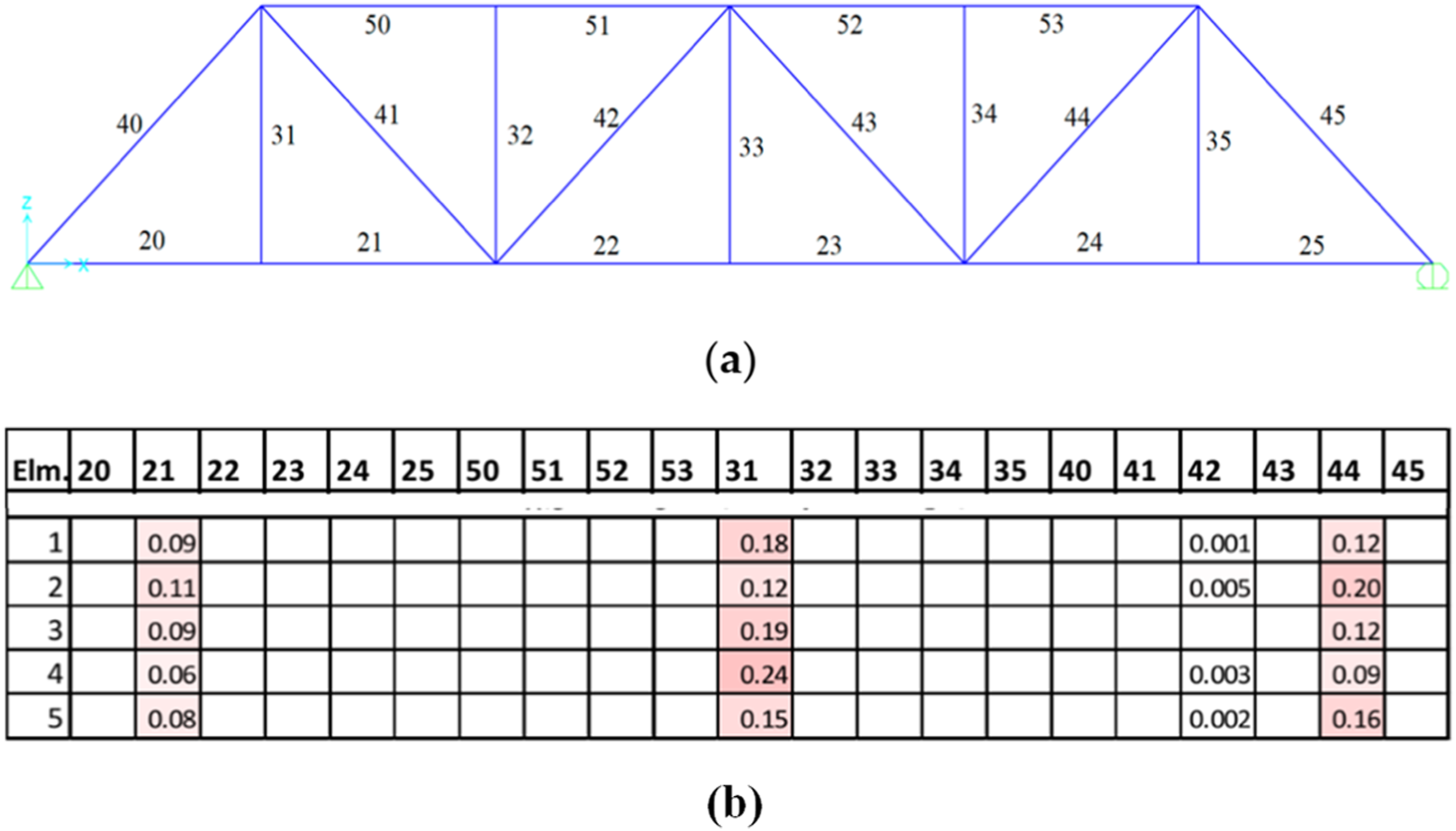
Damage scenario of 20% stiffness loss at bars 21, 31 and 44: (a) Bridge Elements (b) $D F_{A + s}$ to all represented elements (Azim and Gül, 2021).

In Figure 13, the $D F_{A + S}$ metric adeptly identifies and flags the three damaged bars. However, information regarding the severity of damage is lost—indicating that the same degree of stiffness loss may have varying responses in the proposed index. While the results are promising, these approaches have not yet addressed EOV and have not been validated through experimental data. The influence of EOV on ARX and ARMAX coefficients introduces nonlinearities that could subsequently impact FRs, DFs, and even the proposed threshold. As a result, adaptations are necessary to align the methodology with real-world scenarios. Moreover, insights from PCA-based approaches in SHM suggest that the initial principal components retain information about EOV, often discarded during normalization processes (Meixedo et al., 2021, 2022). Therefore, the use of the current framework is highly susceptible to EOVs perturbations.

The discussed damage detection strategies primarily rely on the application of least squares to determine AR coefficients, subsequently leading to the formulation of a damage index. However, alternative strategies exist for coefficient determination. A recent example by Gong et al. (2023) pertains to the detection of settlements in railway bridge piers, using an adapted version of AR models. Rather than employing least squares, they employed a Robust Weighted Total Least-Squares (RWTLS) technique to derive the coefficients of equation (1). This approach leverages the residual error normalized by standard deviation to construct a robust estimator via a weights function.

Subsequently, the authors introduced an Adaptive Dynamic Cubic Exponential Smoothing (ADCES) model. The fundamental premise centers on the notion that extreme values in the time-series introduce randomness that interferes with the established pattern captured and fitted by the time-series model. To enhance the objectivity of methodology, the ADCES initial values and smoothing coefficients were determined through Particle Swarm Optimization. These values were further dynamically adapted across the dataset via Optimal Nonnegative Variable Weight Combination.

An application of this framework was made to pier settlements in the Xi’an–Chengdu high-speed railway in China. The dataset comprised three sets of 20 weekly observations for the years 2014 and 2015. The first 10 observations were used as training data, while the subsequent 10 were designated for testing. The performance of predictions was evaluated using three error metrics: Mean Absolute Error (MAE), Mean Absolute Percentage (MAP), and Root Mean Squared Error (RMSE). As the authors are creating a predictive model the better model may be associated to the minimum error. The proposed model has a better performance than pure RWTLS-AR, and then ADCES when comparing models’ predictions. The obtained errors of the proposed method were compared with pure ADCES or RWTLS-AR, Discrete Gray Model-Linear Regression (DGM-LR), Gray Model-Autoregressive Integrated Moving Average (GM-ARIMA), and Metabolic Gray Model-Cubic Exponential Smoothing (MGM-CES). The authors methodology presented a reduction of 73.789% in MAE and 78.692% in RMSE. This pattern of enhanced performance carried across all analyzed datasets. However, this predictive model is heavily dependent on the variables considered, such that related to adjustments made to handle outliers and to achieve optimized estimates with limited information. Hence, this framework is not necessarily replicable in other contexts.

While AR and ANN models constitute distinct categories, authors sometimes amalgamate them to create a comprehensive framework for robust damage detection. Zhang et al. (2019) exemplify this approach by employing an Auto Associative Neural Network (AANN) to mitigate the impact of EOV on ARX coefficients, which were used as DSFs for a footbridge. In this novel framework, the AANN’s ability to model nonlinear relationships was leveraged to effectively address EOV-induced disturbances that affect ARX coefficients.

Nonlinear time-series models

Initially, the literature predominantly employed ANN for time-series data under the assumption that the residual errors of a regression ANN would conform to a normal distribution. However, only in recent years studies explicitly sought to incorporate specific architectures that could take advantage of the sequential data structure. Frameworks such as RNNs, GRUs, and LSTMs are examples of this evolving approach within the field of SHM.

A straightforward yet effective approach was developed by Finotti et al. (2019), adopting a supervised methodology. The authors extracted 10 statistical indicators from acceleration responses and used them to train both an ANN and a SVM model. These models were designed for classification, categorizing samples into undamaged or two levels of damage conditions for laboratory data, and subsequently distinguishing between undamaged and damaged states for a railway bridge.

Validation of the proposed methodology was conducted using data acquired from a bridge located on the South-East high-speed track between Sens and Soucy, in France. Data were collected before and after a strengthening procedure, covering a total of 15 tests pre- and 13 post-procedure tests. The measurements captured acceleration responses triggered by the passage of trains. Employing eight vertical and two horizontal accelerometers, the data was sampled. Figure 14 illustrates the sensitivity of statistical moments to damage.

Figure 14.

Statistical moments of accelerations responses before and after strengthening (Finotti et al., 2019).

Given that the specific values were not provided, the results presented in Figure 14 do not provide the necessary granularity to discern which statistical moments are most sensitive to damage—thus making it impossible to identify the optimal feature. However, it is important to note that these statistical indicators are employed only as inputs for subsequent classifiers within the methodology. To the classification aspect, the ensuing confusion matrices are displayed succinctly in Figure 15(a) and (b).

Figure 15.

Confusion matrices before and after strengthening for: (a) ANN (b) SVM (Finotti et al., 2019).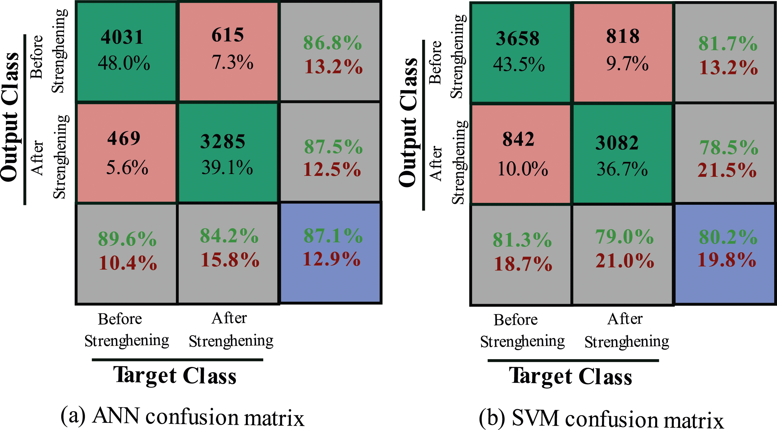

Figure 15 provides a depiction of the outcomes, encompassing the true positive and negative rates, as well as the false positive and negative rates pertinent to the classification task. The accuracy metric, situated in the blue quadrant, attains a commendable 87.1%, accompanied by an error rate of 12.9%. While accuracy gives an average evaluation of a classifier’s performance, a more detailed and comprehensive analysis can be achieved through the consideration of diverse metrics. Similarly, the error rate, while informative, lacks the granularity to distinguish between different types of errors.

For a more comprehensive evaluation, various metrics that are not in the paper, such as recall, precision, F1-score, and the area under the curve (AUC) were calculated and are presented in Table 4. This assessment provides a broader understanding of the classifier’s behavior, accounting for not only the errors but also the specific nuances associated with Type I and Type II errors, and ultimately informing decision-making processes in the context of condition assessment and maintenance planning.

Table 4.

Classification Metrics for ANN and SVM.

Accuracy	Precision	Recall	F1-score	AUC
ANN
87.10%	89.58%	86.76%	88.15%	0.8423
SVM
80.24%	81.29%	81.72%	81.51%	0.7905

With the Type I and Type II errors closely aligned, the other metrics exhibit relatively minor fluctuations. Although recall slightly trails accuracy, precision shows a marginal increase. This divergence in precision and recall signifies that the classifier tends to erroneously assign a greater number of Type II errors—precisely the opposite of the desired outcome concerning safety considerations. However, the F1-Score, which summarizes the information from precision and recall into a single score, reflects an overall satisfactory performance. This metric is particularly valuable, as it offers a balanced assessment that is more fitting than a simple arithmetic mean (as seen in accuracy), revealing issues in either precision or recall. The corroborating results from the Area Under the Curve (AUC) confirm these findings and provide a clearer perspective, ultimately underscoring the superior performance of the ANN. Finally, given that strategies employing binary classification often have limited information for damaged states, other metrics suitable for imbalanced datasets, such as PR-AUC or Cohen Kappa, could be used.

The outlined approach employed both SVM and ANN to address a supervised classification problem. An alternative use involves defining a predictive model for responses, wherein the prediction errors may be used as DSF. A regression-based ANN methodology is exemplified by Chalouhi et al. (2017). In this study, the authors proposed a method for damage detection in a railway bridge using accelerations and temperature measurements as inputs. The collected data, covering both reference and current conditions, was preprocessed to extract pertinent attributes such as running direction, speed, and axle count, thereby facilitating grouping of the training dataset and identification of the most prevalent vehicle type. Subsequently, the ANN was trained to simulate the bridge’s acceleration responses under varying speeds for the predominant train type. The prediction error ( $p e^{s}$ ) was then calculated using equation (28):

p e^{s} = \frac{1}{n} \sum_{i = 1}^{n} {[A N N (x_{i}^{s}) - a_{i}^{s}]}^{2}

(28)

Where

n

is the number of time steps considered in each train passage,

A N N (x_{i}^{s})

is the predicted acceleration after training with data from reference condition,

a_{i}^{s}

is the measured acceleration. In sequence, the authors introduced a Gaussian process to stochastically characterize

p e^{s}

. Finally, a damage index (DI) is computed by equation (29):

D I = \frac{1}{n_{s}} \sum_{s = 1}^{n_{s}} \frac{{p e}^{s} - μ_{s} (\bar{v})}{σ_{s} (\bar{v})}

(29)

Where

n_{s}

is the number of accelerometers installed on the bridge,

μ_{s}

is the mean of

p e^{s}

σ_{s}

is the standard deviation, and

\bar{v}

is the velocity of the train. DI as defined on equation (29), is a normalized distance per velocity, which is expected to increase as the prediction error increase due to presence of abnormality. Figure 16 exhibits the DI results per train passage.

Figure 16.

DI per train simulation to reference condition (in blue) and altered condition (red) (Chalouhi et al., 2017).

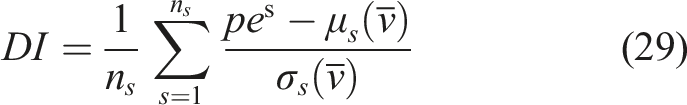
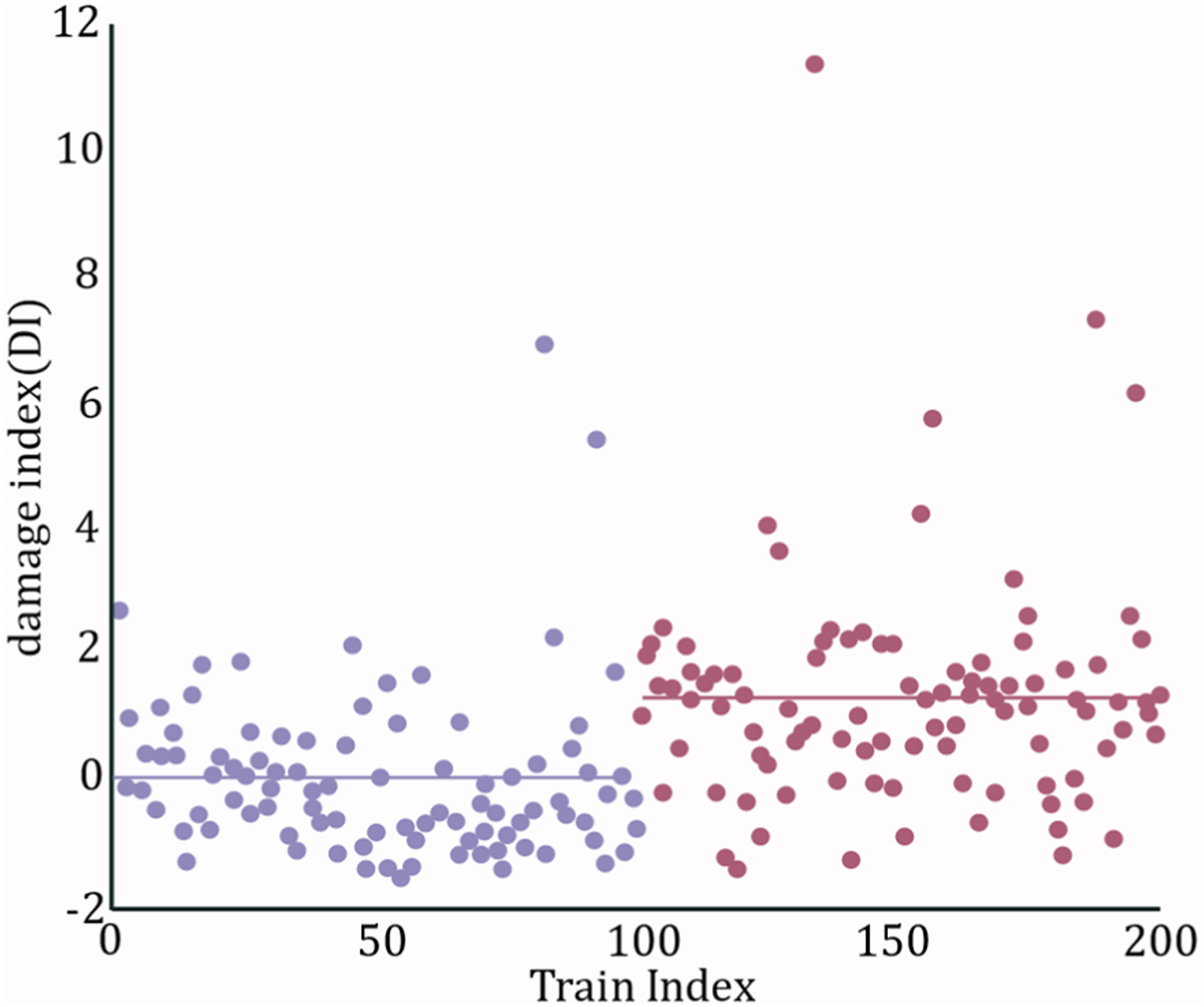
Figure 16 shows discrepancies between the reference condition (blue) and the current condition (red). Meanwhile the AUC, which serves as an indicator of a classifier’s effectiveness, yielded a satisfactory value of 0.7786. Nevertheless, information regarding the selection of the model’s hyperparameters, as well as other pertinent metrics for the binary classification problem, were not presented. This compromises the ability to analyze the model’s performance, as the adopted isolated indicators do not allow for the discernment of issues such as overfitting, or whether the classifier’s performance is equivalent to a random classifier solely based on frequency of the samples.

A distinct study was presented by Santos et al. (2016), introducing an unsupervised and online framework for damage detection. This approach leverages rotations, displacements, and temperature measurements collected from a sensor network on an hourly basis to train an ANN. For each attribute, residual errors were derived by subtracting measured data from predicted values. By virtue of the ANN’s capacity to capture nonlinear relationships, it effectively accounts for the influence of EOVs.

Subsequently, numerous damage scenarios were simulated by introducing stiffness reductions in a FEM of the railway bridge. The model was tri-dimensional with 404 beam elements. According to the authors, the model’s geometry reproduced the original design drawings, and the boundary conditions were defined according to the results obtained from geotechnical tests conducted during the construction. The model was calibrated using real measurements, until displacements and rotations responses with the added noise, were equivalent to those acquired in situ.

The authors employed the dataset from each damage scenario in its entirety, aiming for the methodology to be entirely unsupervised. However, this approach increases the risks of overfitting, thereby diminishing the applicability of the results to other structures.

Separate ANNs were trained for each of the stiffness reductions. Employing the k-means clustering method, the authors determined the optimal number of partitions based on the highest value of the global silhouette index (SIL) and calculated the dissimilarity among the various partitions (DC). The dissimilarity between a reference and damaged cluster is expected to increase. Thus, this feature allows statistical discrimination.

A CB was established under the assumption of a normal distribution for DC. Finally, an index was devised based on the relationship between DC and CB. This index effectively indicates whether a feature’s behavior is within the confidence boundary (implying no damage) or falls outside (indicating potential damage). Figure 17 illustrates the false detection rate—a ratio between incorrectly and correctly assigned statuses—while varying the number of days considered for training the ANN.

Figure 17.

False Detection rate of the strategy proposed by Santos et al. to several stiffness reductions values (Santos et al., 2016).

The methodology was efficient in detecting stiffness variations as subtle as 1% within the context of simulated damaged scenarios, to the tailored problem. However, the model could benefit from hyperparameter optimization, instead of fixing it, using other metrics for performance, and cross validation, to assure the capability of generalization, essential to a damage detection model to real world application.

Neves et al. (2018) introduced an unsupervised approach for ANN-based damage detection, employing a FEM encompassing bridge deck, two steel girders, steel cross bracings, and a single track to represent a generic railway bridge. The girders and deck were modeled as shell elements, and cross bracings as bar elements. All connections among the elements were modeled as rigid. The study considered two distinct damage scenarios: The first damage scenario simulated the removal of a section of the bottom flange of one girder beam; the second scenario consisted of the removal of one bracing. For the former, the modelling intended to reproduce a damage situation where fatigue crack exists, for the later, to reproduce a situation where there is looseness in the bolted connection. This analysis comprised 300 simulations of train crossings, with speeds ranging from 70 to 100 km/h in 0.1 km/h increments. The acceleration responses were used to train an ANN. Subsequently, the RMSE was computed using equation (30), thereby serving as metric to gauge the predictive performance of the trained model.

R M S E = \sqrt{\frac{\sum_{i = 1}^{T} {({output}_{i} - {target}_{i})}^{2}}{T}}

(30)

Where

o u t p u t_{i}

is the

i t h

value predicted by the trained ANN,

t a r g e t_{i}

is the measured value and

T

is the time interval among each measurement. Next, a gaussian process was done in the RMSE. Then, the authors discriminate the structure condition considering a DI equivalent to equation (30), that only differs from Chalouhi et al. (2017) in respect to the error metrics used, considering that authors used RMSE instead of

p e^{s}

. Therefore, the authors considered this error as a DSF, expected to change in the presence of damage. The evaluation of statistical classification results focused exclusively on the ROC curve. However, comprehensive details about classification metrics such as the confusion matrix, and subsequent metrics were omitted. Furthermore, the absence of an application to an experimental dataset makes it less feasible for the proposed methodology to work properly in a real-world scenario.

Ghiasi et al. (2022) used a CNN-based model to not only detect damage but also assess its severity. Initially, the authors constructed a FEM of the Callington Railway bridge constituted by beam elements to the steel beams, and shell elements for the concrete slab. The FE model undergoes excitation through a load characterized by a Gaussian white noise random matrix, as referenced in Parisi et al. (2022), aiming to simulate the bridge’s natural vibrations after the passage of the train. The time step for the transient analysis was chosen by a sensitivity analysis. The calibration of this FEM was achieved using accelerations measured on site. Subsequently, the authors simulated 255 damage scenarios with both unnoisy and noisy conditions with various signal-to-noise ratios (SNR), added for considering measurements disturbances. In essence three different corrosion levels, each inducing cross-sectional losses of 10%, 20%, and 40%, distributed across various locations along with varying noise conditions. This cumulative effort led to a total of 256 distinct damage scenarios. Each simulation had six vectors of acceleration values spanning 1300-time steps, captured at a temporal resolution of 0.0015 s.

Leveraging this dataset, a CNN was trained to distinguish between damaged and undamaged states while also measuring the severity of the damage. Figure 18 illustrates the classification outcomes for the simulated damage scenarios.

Figure 18.

Classification results to minor, moderate, and heavy damage levels (Ghiasi et al., 2022).

The accuracy results for damage detection are along the green diagonal, exhibiting an achievement of 99.51%. A high accuracy is reflected in these outcomes. Remarkably, only a single error was observed in terms of damage level classification, where a minor damage instance (10% cross-sectional loss) was wrongly labeled as moderate (20%). However, as previously mentioned, accuracy is a generalist indicator, unsuitable for identifying issues related to the methodology that would compromise its application with different data sets.

A presentation technique employed to show the classifier’s outcomes is the implementation of a t-Distributed Stochastic Neighbor Embedding (t-SNE). This algorithm facilitates the projection of feature vectors, extracted by the CNN, onto a two-dimensional plane. The result is a visually intuitive representation that enables effective data visualization. This novel visualization approach is exemplified in Figure 19, offering a useful way to visualize the distribution and separation of data points within the two-dimensional space.

Figure 19.

CNN features vector projected into a 2D space (Ghiasi et al., 2022).

The projection visually demonstrates CNN’s ability to accurately group simulated damage levels. Despite these promising findings, it is important to note that no real-world data application was conducted, potentially introducing challenges when detailed information about damage extent labeling might not be readily available.

Another efficient CNN-based approach was pioneered by Parisi et al. (2022), using strain data as a basis. The authors created a FEM model of the Quisi Bridge in Valencia, Spain. The trusses were modeled using bar elements, and the stiffening plates as shell elements. In the first span the supports were considered fixed on one end and mobile on another end. Finally, no noise addition was mentioned, and no real data was used to calibrate the model. While adhering to the fundamental steps shared by many of the frameworks—such as establishing a FEM of a railway bridge, defining damage scenarios and locations—the authors introduced a novel development by engaging in feature selection. This strategic selection aimed to retain only pertinent information through the application of a distance-based machine learning algorithm.

In this method, a Kth Nearest Neighbor Algorithm (KNN) was deployed for each damage scenario, with the accuracy metric serving as a determinant of a sensor’s utility in condition assessment. Given the utilization of time-series data, the authors introduced Dynamic Time Warping (DTW) in conjunction with KNN to ascertain the optimal number of sensors for achieving the highest accuracy. Subsequently, this acquired knowledge was employed to train a dedicated CNN for each damage scenario.

Reference responses were obtained by subjecting the FEM of the bridge to controlled conditions. Among all bridge elements, 10 were randomly selected, and three levels of damage were systematically applied to each of these elements via the FEM representation. The feature selection procedure, characterized by KNN and DTW, returned a critical value of elements for KNN ( $r$ ) as either 3 or 4. Figure 20 depicts the confusion matrix, wherein the accuracy scale is visually accentuated, under two scenarios: $r = 4$ (a) and $r = 12$ (b).

Figure 20.

Confusion matrix with accuracy for (a) 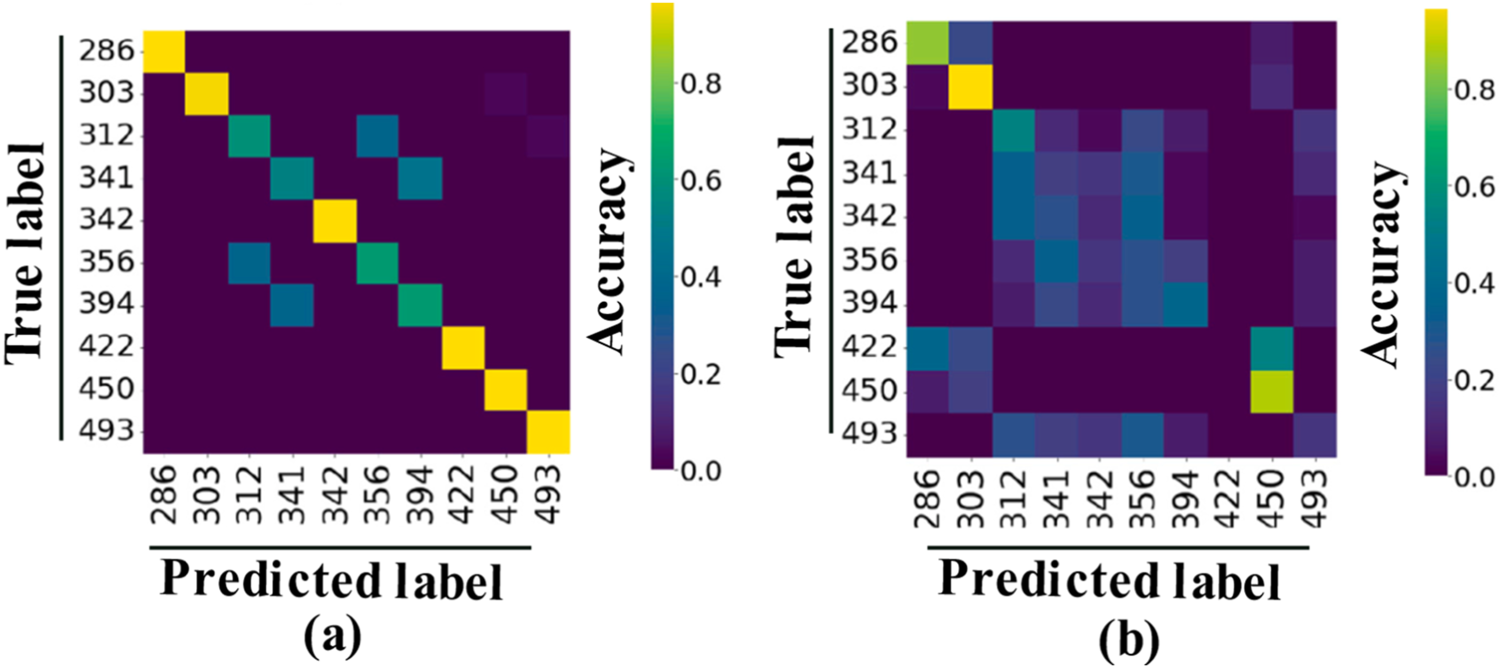$r = 4$ (b) $r = 12$ (Parisi et al., 2022).

Figure 20 effectively illustrates the impact of incorporating a varying number of sensors in a classification context, specifically in terms of accurately identifying the selected elements as damaged. In Figure 20(a), there is remarkably reduced dispersion of points (with nearly all data points aligned along the diagonal) and consequently high accuracy. On the contrary, for $r$ = 12, the inclusion of data from additional sensors leads to increased scattering and diminished accuracy, as depicted in Figure 20(b). Thus, this analysis firmly establishes that using four sensors emerges as the optimal choice to train a CNN, ensuring high accuracy while employing a streamlined dataset.

Following the feature selection phase, CNNs were trained for both

r = 3

and

r = 4

. Given the supervised nature of the machine learning approach employed by the authors, their assessment primarily focused on damage localization and severity estimation. These results are summarized in Table 5.

Table 5.

DL and DA Assessment (Parisi et al., 2022).

r	Damage location (DL)				Damage severity assessment (DA)
r	CNN	Accuracy (%)	1NN-DTW	Accuracy (%)	CNN	Accuracy (%)	1NN-DTW	Accuracy (%)
r = 3	$C N N_{3}$	93	$m_{3}$	84	$C N N_{3}$	73	$m_{3}$	56
r = 4	$C N N_{4}$	91	$m_{4}$	84	$C N N_{4}$	75	$m_{4}$	55

Table 5 provides a comprehensive overview of the accuracy achieved through the KNN-DTW feature selection process for each hierarchical level: Damage Location (DL) and Damage Severity (DA). The methodology demonstrated adequate ability to accurately pinpoint damage based on pre-selected data. In terms of severity assessment, although feature selection does not have exceptionally high values, the CNN still produces satisfactory accuracy metrics. The main limitation lies in the requirement for information about damage severities and locations, which is typically not readily available in real-world applications. As CNN is adept at capturing nonlinear relationships, the impact of EOV may not significantly disrupt the effectiveness of the proposed method. By its very nature, the method deals with overfitting by restraining its training set. Thus, analyze other metrics could allow to better understand the potential of the method. Additionally, the FEM was not calibrated with real data. As the approach rely on it to generate information, this compromises real world applications.

A recent application (Han et al., 2019) employed the NARX model to characterize train-bridge responses with the aim of predicting accelerations on the bridge. The architecture comprises 10 nodes within the hidden layer, with a sigmoid activation function and MSE as the loss function. To emulate track irregularities, the authors created a FEM to the bridge consisting solely of beam elements to girders and piers. No information regarding constraint were presented. To the train, a nonlinear 2-DOF system representing a quarter-vehicle model of vehicle suspension was used. Based on a German high-speed railway spectra, the authors generated 10,000 stochastic excitations. Subsequently, a bridge was simulated with track irregularities, featuring a train speed of 200 km/h. A total of one thousand simulations were carried out, and the outcomes present adequate predictions to the irregularities simulated.

Despite the absence of explicit metrics, the presentation of a relative error of the order of $4 \times 10^{- 2}$ underscores the exceptional performance of the methodology. Even though there was no EOV discrimination process the adequate results attest how this nonlinear model is flexible and capable for effectively characterizing and predicting anomalies within time-series data from railway bridges. A better understanding of the models’ capabilities would be available if other errors as MAE, MAP and MSE were presented. Additionally, predictions models are highly dependent on the parameters inserted. Hence, an hyperparameter optimization would be crucial, as NARX are able to capture long term time patterns to different signals, making feasible to applications to new data. Within the ANN-based time-series analysis, contemporary investigations are prominently linked with LSTM networks, primarily due to their capacity for predicting responses via complex nonlinear combinations (Han et al., 2019). This feature results in higher sensitivity to damage. A case in point is the work of Wang et al. (2022), who introduced a condition assessment approach employing LSTM applied to temperature and deflection data. The initial step involves normalizing the collected data using equations (31) and (32):

d = \frac{D - C_{\min - d}}{C_{\max - d} - C_{\min - d}}

(31)

t = \frac{T - C_{\min - t}}{C_{\max - t} - C_{\min - t}}

(32)

Where

d

and

t

are the normalized deflections and temperature;

D

and

T

are the measured deflections and temperature;

C_{\max - d}

and

C_{\min - d}

C_{\max - t}

and

C_{\min - t}

are the scaling parameters for deflections and temperature, respectively.

C_{\max}

and

C_{\min}

are the maximum or minimum of the normalizing parameter. The normalization is a well-known practice when dealing with several inputs with different scales, which might influence the weights during the training.

The normalized data was introduced in the LSTM, with optimized parameters. As a small learning rate increases the computational costs and a higher generates an unstable convergence process, determining the optimum value is a crucial task concerning big data. The authors employed grid search to determine the hyperparameters, which is a high computational cost yet efficient method. However, there is no description of isolated optimization process for each input variable. This would be the better scenario due to the different pattern that displacements and temperature exhibit on time. One option to reduce the inherent higher computational cost of this approach is to use gradient-based hyperparameter search. After training, the squared error index (SE) was obtained by equation (33):

S E = {(o u t p u t_{i} - t a r g e t_{i})}^{2}

(33)

Next, since errors are expected to change in the presence of damage, hypothesis tests were conducted to determine the differences between the current condition and the reference condition. In sequence, data collected from deflections and temperature of the Chongqing Egongyan Rail Transit Bridge over 15 months was used to establish the baseline. As damage scenario measurements were not available, a FEM was used to obtain data for different cable cross-section reduction of 0.3, 0.5, 1.0, 1.5, 2.0, and 2.5%. The authors presented no details about the modelling of the bridge.” The authors presented no detailing about the modelling of the bridge. After, a right-tail $t$ -test was used to identify whether baseline SE and damaged SE were equivalent ( $H_{0}$ ) or not ( $H_{1}$ ), that infers that damage causes the increasing of t statistic. The findings of the study show the effectiveness of the methodology in locating damage in the mid-span, capable of detecting stiffness losses as low as 0.5% when accounting for two cables. At L/4 and L/8 positions, the corresponding minimum detectable cross section reductions were 1.0% and 2.5%, respectively. This observation shows the sensitivity of the error metrics with respect to the precise location of the damage. A similar trend was observed in scenarios where only a single cable was damaged.

A correlation emerged between the modeled stiffness loss and the t-value, reflecting a positive relationship. This correlation has a dual advantage, enabling both qualitative and quantitative assessments of damage severity. Consequently, the framework holds the potential to establish a robust early warning system. To further elucidate the methodology’s performance in the context of the lowest detected damage level (0.5%), an in-depth analysis of accuracy metrics was conducted. The findings reveal an accuracy exceeding 75% when using data spanning more than 30 days. Moreover, an intriguing aspect was explored by exclusively employing deflection data for training the LSTM model. This approach succeeded in detecting damages with a cross-sectional reduction as little as 1%. However, crucial evaluation metrics such as Type-I and Type-II errors, as well as precision, recall, F1-score and F2-score that could be provided, as the framework is a binary classifier problem, were regrettably not provided, hindering a comprehensive analysis of this approach. Also, the application of the framework to benchmark datasets would grant further evidence regarding the robustness of the method.

A LSTM-based strategy was introduced by Yue et al. (2021), centered around deflection and temperature deflection data from a combined highway and railway cable-stayed bridge situated over the Yangtze River. After establishing the correlation between temperature and deflection to the collected data, the researchers proceeded to train an LSTM model on the initial 75% of the dataset. Subsequently, deviations spanning from 0.25% to 2% were introduced into the final 25% of the dataset to assess the model’s ability to identify anomalies.

The t-test was used to verify if the LSTM model’s predictions to damaged and undamaged scenarios presented a different distribution. On this statistical hypothesis testing, the null hypothesis ( $H_{0}$ ) states that two variables, such as normal and damaged data, are statistically equivalent, while the alternative hypothesis ( $H_{1}$ ) posits that they are different. The conducted tests exhibited the capability to detect deviations as minimal as 0.3%, predicated on the LSTM parameters. However, it’s important to clarify that a 0.3% inserted deviation does not necessarily equate to other usual damage modelling such as cross section reduction or stiffness loss. The distinction arises from the fact that stiffness or cross section reduction exert only an indirect influence on the dataset. Consequently, a direct deviation in the dataset may be comparatively easier to identify than the previous damage models. Furthermore, such generalized deviation might not correspond to real world scenarios, compromising the application of such approach.

Other applications of linear and nonlinear models

Certainly, linear, and nonlinear models have versatile applications within the field of SHM. For instance, Al-Zuriqat et al. (2023) introduced a fault detection framework known as Adaptive Fault Detecting based on Analytical Redundancy (AFDAR), which combines MA processes with ANN. In this methodology, a designated output point is chosen within a sensor network, and an ANN is trained using acceleration measurements from correlated sensors to predict responses at that point. The predicted outputs from the ANN are then compared to the actual data from the single sensor until a predefined threshold for damage detection is met. Employing MA processes, if a particular sensor is consistently flagged with faults within each time window, the ANN stop using data from that sensor to prevent compromising the framework. However, this approach relies on engineering judgment to establish the threshold, relying on professional expertise.

In a similar vein, He et al. (2016) integrated ARIMA models into an early warning system designed to predict abutment settlements on the Tiajin-Beijing railway bridge during the construction of the Cuiheng Road Underpass. By utilizing 2 years’ worth of data, the authors forecasted abutment settlements for the subsequent 3 months. By that, is possible to infer a model order of 24. However, no detail regarding the criteria used to establish it was given. A non-optimized model order may lead to overfitting. The proposal model achieved an error of only 1% in relation to the targeted period (the third month). The authors do not inform whether they use true targets, that is, if for the second and third prediction they used the predicted or the true value. Furthermore, the authors established thresholds based on errors of prediction regarding the theoretical values for two levels of warning. However, the predictions are highly dependent on the models’ hyperparameter values. Without an objective way of establishing it, there is no guarantee that the predictions would keep the same average error. Finally, the authors do not state if there was any warning active during the monitoring time.

In conclusion, for all the time-series models applied to railway bridges that were extensively discussed, the models used, the main results, and the origin of the data used to train the models are shown in Table 6.

Table 6.

Discussed papers models, main results and data precedence.

Authors	Models	Main results	Data precedence
Azim (2021)	ARMAX	Adequate damage detection achieved to stiffness loss as low as 10%. Information regarding location and severity was obtained	FEM
Chalouhi et al. (2017)	ANN	Adequate damage detection achieved with AUC = 0.7786	Monitoring
Meixedo et al. (2022)	ARX	Adequate damage detection achieved to stiffness loss of 5% with less than 2% Type-I error using 19 train passages	FEM/Monitoring
Azim and Gül (2021)	AR	Adequate damage detection achieved to stiffness loss of 10%. Information regarding location at element level was obtained	FEM
Wang et al. (2022)	LSTM	Adequate damage detection achieved to cross-section reduction of 0.5% with 100% accuracy when information of more than 31 days was used. Information about severity was obtained.	FEM/Monitoring
Meixedo et al. (2021)	AR	Adequate damage detection achieved to stiffness loss of 5% with 1% Type-I error	FEM/Monitoring
Santos et al. (2016)	ANN	Adequate damage detection achieved to stiffness loss of 1% to simulated data.	FEM/Monitoring
Parisi et al. (2022)	CNN	Adequate damaged detection and localization assessment with accuracy over 90%. Severity information obtained with accuracy over 75%.	FEM/Monitoring
Azim and Gül (2019)	ARX	Adequate damage detection achieved to stiffness loss as low as 10%. Information regarding location and severity was obtained	FEM
Mei and Gül (2016)	AR	Adequate damage detection achieved to stiffness loss as low as 10%. Information regarding location and severity was obtained	FEM
Gong et al. (2023)	AR	Adequate damage prediction with RMSE = 0.101	Monitoring
Neves et al. (2018)	ANN	Adequate damage detection achieved to different I of bracings removal	FEM
Han et al. (2019)	NARX	Adequate damage detection able to detection track irregularities with relative error of $4 x 10^{- 2}$	FEM
Yue et al. (2021)	LSTM	Adequate damage detection achieved to inserted accelerations deviations of 0.3%	FEM
He et al. (2016)	ARIMA	Adequate damage prediction with relative error of 1%	Monitoring
Ghiasi et al. (2022)	CNN	Adequate damage detection and severity assessment achieved to 10% cross-sectional loss	FEM
Finotti et al. (2019)	ANN	Adequate damage detection with accuracy of 87.1%	Monitoring

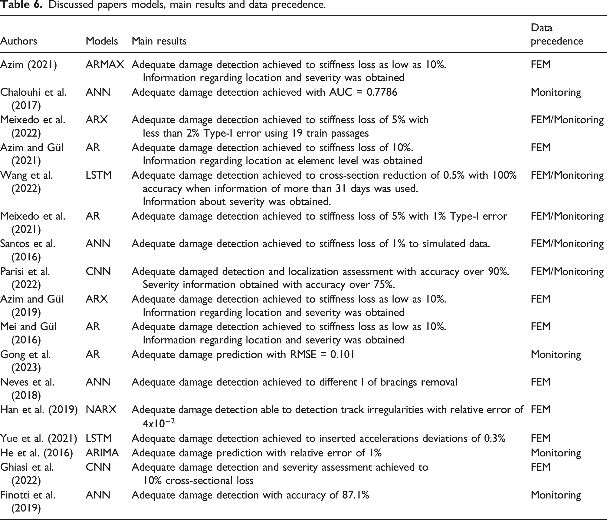
The table highlights the main results, emphasizing the damage detection hierarch level and the type of data used, which is relevant to analyze the robustness of the methodologies. The selected studies offer a comprehensive overview of the possibilities for using time series models. Among the analyses woven throughout the text, emphasis is placed on the scant consideration of the influence of EOVs, the need for both hyperparameter optimization, and the evaluation of results obtained in the models. For example, fixing model order may not allow to the model learn the patterns along time properly. For the evaluation metrics, while accuracy is widely prevalent across various works, this indicator is generalist and does not allow for a complete characterization of the model. It is necessary to understand how and where the model is right or wrong, as well as if it is generalist enough to work on new data.

Conclusions

This article presents and discusses linear and nonlinear time series models, analyzing their application in the assessment of the condition of railway bridges. The development of these models has enabled more effective utilization of collected data due to their flexibility, ease of application, and capacity to retain relevant information. Both linear and nonlinear models have demonstrated their robustness and efficacy in diagnosing damages in railway bridges, even allowing for the extraction of location and severity information from collected data. However, further studies are needed to consolidate these methodologies for practical integration into SHM systems.

As discussed, models trained to predict time responses exhibit sensitivity to both damage and variations in train loads, speed, and environmental conditions. An appropriate analysis should observe how the employed model responds to external factors, including additional normalization processes when necessary. In this context, the article emphasizes the effectiveness of linear models when used within an appropriate strategy and the intrinsic capability of nonlinear models to handle these external factors.

Despite the recent advancements presented, most studies rely on simplified numerical models that are inadequate to represent the complexity of railway bridge responses and the variability of various loading conditions. Application in real-world scenarios would require a verification of the robustness and sensitivity of the methodology, as well as to optimize model hyperparameters to balance computational cost and performance, capturing the underlying time-patterns adequately.

Numerous steps can be taken to further develop this field. Initially, greater utilization of various forms of linear models is suggested to consolidate application methodologies. In their architecture, different levels of diagnosis and susceptibility to environmental and operational variations should be extensively evaluated. Different model order choosing criteria could be explored, comparing performance and computational cost. When dealing with exogenous models the cluster techniques tend to be the same. However, as computational capabilities are growing, different techniques must be tried, for example, optimize the model order for each exogenous sensors, using KNN as information selection criteria, among others.

Similarly, a deeper understanding of nonlinear models is required. This class is capable of learning complex response patterns, modeling environmental and operational influences without additional inputs, with higher sensitivity. Subsequently, extensive studies should be conducted, assessing the trade-off between computational cost and the hierarchical level of the damage detection strategy, aiming for optimized allocation of methodologies and resources.

Finally, since these methods are data-driven, consolidation as a practical tool for SHM must involve application to real collected data from railway bridges, with metrics that allow to completely characterize the framework performance to the study and to new data.

Footnotes

Declaration of conflicting interests

The author(s) declared no potential conflicts of interest with respect to the research, authorship, and/or publication of this article.

Funding

The author(s) disclosed receipt of the following financial support for the research, authorship, and/or publication of this article: The first author was financially supported by Fundação Coordenação de Aperfeiçoamento de Pessoal de Nível Superior (CAPES) under grant number 88887.816768/2023-00 and Fundação para o Desenvolvimento Tecnológico da Engenharia (FDTE) on the project 1924. The first and the fourth authors integrates the research project “Inspeção e Monitoramento de Obras de Arte Especiais por meio de Técnicas Remotas e não Invasivas” of Cátedra Under Rail - VALE. The second and third authors were financially supported by: Base Funding - UIDB/04708/2020 with DOI 10.54499/UIDB/04708/2020 (https://doi.org/10.54499/UIDB/04708/2020) and Programmatic Funding - UIDP/04708/2020 with DOI 10.54499/UIDP/04708/2020 (https://doi.org/10.54499/UIDP/04708/2020) of the CONSTRUCT - Instituto de I&D em Estruturas e Construções - funded by national funds through the FCT/MCTES (PIDDAC).

ORCID iD

Igor Ribeiro

References

Ahmed

Atiya

El Gayar

, et al. (2010) An empirical comparison of machine learning models for time-series forecasting. Econometric Reviews 29(5): 594–621. DOI: 10.1080/07474938.2010.481556.

Alves

Cury

Cremona

(2016) On the use of symbolic vibration data for robust structural health monitoring. Proceedings of the Institution of Civil Engineers: Structures and Buildings 169(9): 715–723. DOI: 10.1680/jstbu.15.00011.

Al-Zuriqat

Chillón Geck

Dragos

, et al. (2023) Adaptive fault diagnosis for simultaneous sensor faults in structural health monitoring systems. Infrastructures 8(3). DOI: 10.3390/infrastructures8030039.

Azim

(2021) A data-driven damage assessment tool for truss-type railroad bridges using train induced strain time-history response. Australian Journal of Structural Engineering 22(2): 147–162. DOI: 10.1080/13287982.2021.1908710.

Azim

Gül

(2019) Damage detection of steel girder railway bridges utilizing operational vibration response. Structural Control and Health Monitoring 26(11): 1–15. DOI: 10.1002/stc.2447.

Azim

Gül

(2020) Damage detection framework for truss railway bridges utilizing statistical analysis of operational strain response. Structural Control and Health Monitoring 27(8): 1–17. DOI: 10.1002/stc.2573.

Azim

Gül

(2021) Development of a novel damage detection framework for truss railway bridges using operational acceleration and strain response. Vibration 4(2): 422–443. DOI: 10.3390/vibration4020028.

Bui-Ngoc

Nguyen-Tran

Nguyen-Ngoc

, et al. (2022) Damage detection in structural health monitoring using hybrid convolution neural network and recurrent neural network. Frattura Ed Integrita Strutturale 16(59): 461–470. DOI: 10.3221/IGF-ESIS.59.30.

Chalouhi

Gonzalez

Gentile

, et al. (2017) Damage detection in railway bridges using Machine Learning: application to a historic structure. Procedia Engineering 199: 1931–1936. DOI: 10.1016/j.proeng.2017.09.287.

10.

Datteo

Busca

Quattromani

, et al. (2018) On the use of AR models for SHM: a global sensitivity and uncertainty analysis framework. Reliability Engineering and System Safety 170(September 2017): 99–115. DOI: 10.1016/j.ress.2017.10.017.

11.

Entezami

(2021) Structural Health Monitoring by Time Series Analysis and Statistical Distance Measures. Cham: Springer. DOI: 10.1007/978-3-030-66259-2.

12.

Entezami

Shariatmadar

(2019) Damage localization under ambient excitations and non-stationary vibration signals by a new hybrid algorithm for feature extraction and multivariate distance correlation methods. Structural Health Monitoring 18(2): 347–375. DOI: 10.1177/1475921718754372.

13.

Farahani

Penumadu

(2016) Damage identification of a full-scale five-girder bridge using time-series analysis of vibration data. Engineering Structures 115: 129–139. DOI: 10.1016/j.engstruct.2016.02.008.

14.

Farrar

Worden

(2012) Structural Health Monitoring: A Machine Learning Perspective. West Sussex: John Wiley & Sons.

15.

Figueiredo

Park

Farrar

, et al. (2011) Machine learning algorithms for damage detection under operational and environmental variability. Structural Health Monitoring 10(6): 559–572. DOI: 10.1177/1475921710388971.

16.

Finotti

Cury

Barbosa

Fde S

(2019) An SHM approach using machine learning and statistical indicators extracted from raw dynamic measurements. Latin American Journal of Solids and Structures 16(2): 1–17. DOI: 10.1590/1679-78254942.

17.

Ghiasi

Moghaddam

, et al. (2022) Damage classification of in-service steel railway bridges using a novel vibration-based convolutional neural network. Engineering Structures 264(June): 114474. DOI: 10.1016/j.engstruct.2022.114474.

18.

Gomez-Cabrera

Escamilla-Ambrosio

(2022) Review of machine-learning techniques applied to structural health monitoring systems for building and bridge structures. Applied Sciences 12(21): 10754. DOI: 10.3390/app122110754.

19.

Gong

Wang

, et al. (2023) Combined prediction model for high-speed railway bridge pier settlement based on robust weighted total least-squares autoregression and adaptive dynamic cubic exponential smoothing. Journal of Surveying Engineering 149(2): 04023001. DOI: 10.1061/jsued2.sueng-1379.

20.

Grandini

Bagli

Visani

(2020) Metrics for multi-class classification: an overview. DOI: 10.48550/arXiv.2008.05756.

21.

Han

Xiang

, et al. (2019) Predictions of vertical train-bridge response using artificial neural network-based surrogate model. Advances in Structural Engineering 22(12): 2712. DOI: 10.1177/1369433219849809.

22.

Duan

Deng

, et al. (2016) Risk assessment and early-warning system for high-speed railway during the construction and operation of underpass bridges. Journal of Performance of Constructed Facilities 30(1): 1–13. DOI: 10.1061/(asce)cf.1943-5509.0000717.

23.

Xuan

(2015) Statistical moments of ARMA(n,m) model residuals for damage detection. Procedia Engineering 130: 1622–1641. DOI: 10.1016/j.proeng.2015.12.351.

24.

Kitagawa

(2010) Introduction to Time Series Modeling. Boca Raton: CRC Press, Taylor & Francis Group.

25.

Lakshmi

Rama Mohan Rao

(2016) Structural damage detection using ARMAX time series models and cepstral distances. Sadhana – Academy Proceedings in Engineering Sciences 41(9): 1081–1097. DOI: 10.1007/s12046-016-0534-3.

26.

Lawal

V Shajihan

Mechitov

, et al. (2023) An Event-Classification Neural Network Approach for Rapid Railroad Bridge Impact Detection. Sensors (Basel, Switzerland) 23(6). DOI: 10.3390/s23063330.

27.

Lim

Zohren

(2021) Time-series forecasting with deep learning: a survey. Philosophical Transactions of the Royal Society A: Mathematical, Physical and Engineering Sciences 379(2194): 20200209. DOI: 10.1098/rsta.2020.0209.

28.

Luo

Huang

Lei

(2022) Temperature effect on vibration properties and vibration-based damage identification of bridge structures: a literature review. Buildings 12(8): 1209. DOI: 10.3390/buildings12081209.

29.

Matsuoka

Tokunaga

Kaito

(2021) Bayesian estimation of instantaneous frequency reduction on cracked concrete railway bridges under high-speed train passage. Mechanical Systems and Signal Processing 161: 107944. DOI: 10.1016/j.ymssp.2021.107944.

30.

Mei

Gül

(2016) A fixed-order time series model for damage detection and localization. Journal of Civil Structural Health Monitoring 6(5): 763–777. DOI: 10.1007/s13349-016-0196-1.

31.

Meixedo

Ribeiro

Santos

, et al. (2021) Damage detection in railway bridges using traffic-induced dynamic responses. Engineering Structures 238(February): 112189. DOI: 10.1016/j.engstruct.2021.112189.

32.

Meixedo

Santos

Ribeiro

, et al. (2022) Online unsupervised detection of structural changes using train–induced dynamic responses. Mechanical Systems and Signal Processing 165(April 2021): 108268. DOI: 10.1016/j.ymssp.2021.108268.

33.

Neves

González

Leander

, et al. (2018) A new approach to damage detection in bridges using machine learning. In: Lecture Notes in Civil Engineering. Singapore: Springer, Vol. 5, 73–84. DOI: 10.1007/978-3-319-67443-8_5.

34.

Niyirora

Masengesho

, et al. (2022) Intelligent damage diagnosis in bridges using vibration-based monitoring approaches and machine learning: a systematic review. Results in Engineering 16(August): 100761. DOI: 10.1016/j.rineng.2022.100761.

35.

Parisi

Mangini

Fanti

, et al. (2022) Automated location of steel truss bridge damage using machine learning and raw strain sensor data. Automation in Construction 138(April): 104249. DOI: 10.1016/j.autcon.2022.104249.

36.

Rastin

Ghodrati Amiri

Darvishan

(2021) Unsupervised structural damage detection technique based on a deep convolutional autoencoder. Shock and Vibration 2021: 6658575. DOI: 10.1155/2021/6658575.

37.

Santos

Crémona

Calado

, et al. (2016) On-line unsupervised detection of early damage. Structural Control and Health Monitoring 23(7): 1047–1069. DOI: 10.1002/stc.1825.

38.

Sharma

Sen

(2023) Real-time structural damage assessment using LSTM networks: regression and classification approaches. Neural Computing and Applications 35(1): 557–572. DOI: 10.1007/s00521-022-07773-6.

39.

Sonbul

Rashid

(2023) Algorithms and techniques for the structural health monitoring of bridges: systematic literature review. Sensors 23(9): 1–29. DOI: 10.3390/s23094230.

40.

Sun

Shang

Xia

, et al. (2020) Review of bridge structural health monitoring aided by big data and artificial intelligence: from condition assessment to damage detection. Journal of Structural Engineering 146(5): 04020073. DOI: 10.1061/(asce)st.1943-541x.0002535.

41.

Tee

(2018) Time-series analysis for vibration-based structural health monitoring: a review. Structural Durability and Health Monitoring 12(3): 129–147. DOI: 10.3970/sdhm.2018.04316.

42.

Umar

Vafaei

Alih

(2021) Sensor clustering-based approach for structural damage identification under ambient vibration. Automation in Construction 121(September 2020): 103433. DOI: 10.1016/j.autcon.2020.103433.

43.

Vagnoli

Remenyte-Prescott

Andrews

(2018) Railway bridge structural health monitoring and fault detection: state-of-the-art methods and future challenges. Structural Health Monitoring 17(4): 971–1007. DOI: 10.1177/1475921717721137.

44.

Wang

Ansari

, et al. (2022) LSTM approach for condition assessment of suspension bridges based on time-series deflection and temperature data. Advances in Structural Engineering 25(66): 3450–3463. DOI: 10.1177/13694332221133604.

45.

Yan

Elgamal

Cottrell

(2013) Substructure vibration NARX neural network approach for statistical damage inference. Journal of Engineering Mechanics 139(6): 737–747. DOI: 10.1061/(asce)em.1943-7889.0000363.

46.

Yang

Zhang

Chen

, et al. (2020) A hierarchical deep convolutional neural network and gated recurrent unit framework for structural damage detection. Information Sciences 540: 117–130. DOI: 10.1016/j.ins.2020.05.090.

47.

Yang

Zhou

, et al. (2021) A data-driven structural damage detection framework based on parallel convolutional neural network and bidirectional gated recurrent unit. Information Sciences 566: 103–117. DOI: 10.1016/j.ins.2021.02.064.

48.

Yue

Ding

Zhao

(2021) Deep learning-based minute-scale digital prediction model of temperature-induced deflection of a cable-stayed bridge: case study. Journal of Bridge Engineering 26(6): 1–13. DOI: 10.1061/(asce)be.1943-5592.0001716.

49.

Zhang

Gül

Kostić

(2019) Eliminating temperature effects in damage detection for civil infrastructure using time-series analysis and autoassociative neural networks. Journal of Aerospace Engineering 32(2): 1–16. DOI: 10.1061/(asce)as.1943-5525.0000987.

50.

Zinno

Haghshenas

Guido

, et al. (2022) Artificial intelligence and structural health monitoring of bridges: a review of the State-of-the-Art. IEEE Access 10(August): 88058–88078. DOI: 10.1109/ACCESS.2022.3199443.