Risk-based asset management framework for highway retaining wall systems using wireless structural health monitoring data

Abstract

Retaining walls are important structural systems used in the construction of highways. With asset management methods for retaining wall inventories lagging those developed for highway bridges, there is a need to develop risk management methods for these critical structural systems. A major challenge is the vast inventories of retaining walls that asset managers must manage and the inherent limitations of visual inspections. This study proposes an asset management framework for retaining walls based on risk assessments using structural monitoring data. First, a long-term wireless monitoring solution is proposed to measure wall tilt and strain over long periods of time. Second, an analytical framework is developed to separate wall thermal responses from lateral earth pressures responses with the latter used to extract estimated lateral earth pressure distributions. A statistical distribution of lateral earth pressures are used in a reliability assessment of the wall to provide a measure of failure probability that can be combined with failure consequences to estimate asset risk. To illustrate the proposed methodology, a reinforced concrete cantilever retaining wall panel is selected for long-term structural health monitoring. A wireless structural health monitoring system is installed to measure the tilt, strain, and temperature response of the wall continuously over 15 months. The study reveals the wall exhibits strong diurnal and seasonal variations offering insight into wall behavior under operational conditions. Hypothesized levels of corrosion in the steel reinforcement at the base of the wall are explored to estimate the wall reliability. Even under the assumption of 20% reinforcement section loss, the monitored wall was found to have a reliability index well above 3.0.

Keywords

wall system monitoring discrete element reliability index risk assessment

Introduction

The construction of highways in dense urban areas and sloping terrains often requires retaining wall systems. In the United States alone, more than 160 million square feet of new wall area are constructed every year within the national highway and road network (FHWA, 2008). This results in massive inventories of retaining wall structures that must be managed by state and local transportation departments. Over the past 50 years, transportation departments have developed highly effective asset management methods that ensure the safe and cost-efficient operation of their structural assets, especially highway bridges and pavements. These methods include extensive use of visual inspection and in some cases structural monitoring and analytical modeling (Uddin et al., 2013; Yanev, 2007). In the U.S., the Moving Ahead for Progress in the 21st Century Act (MAP-21) passed by Congress requires transportation agencies adopt risk management strategies for all their transportation assets (FHWA, 2014). MAP-21 has transformed how bridges are managed including the use of risk matrices to assign bridges to low-, medium-, and high-risk categories based on failure consequences (FHWA, 2017). Given the success of risk management methods for bridges and pavements, and the recent mandates of MAP-21, transportation agencies are developing risk assessment methods for geotechnical systems including earth retaining structures (Vessely et al., 2019). The first step of geotechnical asset management is the development of databases to store an inventory of earth retaining structures and inspection methods to visually assess system conditions on a frequent time basis.

Today, several transportation agencies across the globe have developed an inventory and inspection program for retaining wall systems (Athanasopoulos-Zekkos et al., 2020). Most of these programs adopt visual inspection methods to assess the physical condition of the retaining wall including the detection of movement and deformation of wall structures and the geotechnical system they support. Inspectors trained in visual inspection methods carry out inspections with primary and secondary wall elements (e.g., structural form, surface coating, backfill material, drainage system, foundation) and assign a condition rating like that done to rate bridge elements. The United States National Parks Service guides inspectors to offer condition narratives for each wall element with a translational framework to map narrative statements to a condition rating between 0 and 10 (DeMarco et al., 2010). Some state agencies like the Nebraska Department of Roads (NDOR) and Colorado Department of Transportation (CDOT) use a rating system identical to what is used for bridges assigning a 0 to 9 rating (Jensen, 2009; Walters et al., 2016) while others like the Oregon Department of Transportation (ODOT) simplify their ratings into “good”, “fair”, and “poor” ratings (ODOT, 2007). Visual inspection intervals range from every 2 years as in the case of VicRoads in Australia (VicRoads, 2014) to every ten years as is the case with the US National Park Service (DeMarco et al., 2010); but 5 years is the most common interval (e.g., Alaska, New York City, Oregon, Pennsylvania). While inventory and inspection programs are an essential step toward the development of risk assessment methods for retaining wall structures, alone they are not sufficient due to the lack of quantitative data required to accurately assess the risk inherent to a retaining wall system using information specific to its in-situ performance. Only structural monitoring can offer quantitative evidence of retaining wall in-situ performance.

With structural monitoring evolving into a cost-effective tool for monitoring the performance and condition of bridges (Flanigan et al., 2020; Frangopol et al., 2008; Fujino and Siringoringo, 2011; Zonta et al. 2007, 2014), asset managers responsible for retaining walls have more recently explored monitoring methods to assist them. Most data collection methods focus on assessing the movement of walls. Manually applied surveying methods such as the use of total stations and global positioning system (GPS) receivers are widely used to measure wall movements over time. Vehicle-mounted sensors including GPS, laser scanners, and cameras have also been explored to offer a more efficient approach to spatially mapping retaining wall geometries with repeated surveys used to track long-term wall deformations (Kalenjuk et al., 2019; Yen et al., 2011). Specifically, LiDAR and photogrammetry offer three-dimensional point cloud data sets with sub-centimeter resolutions (Kim et al., 2009; Oskouie et al., 2016). Mobile mapping methods based on LiDAR have been validated to accurately map 150 linear miles of wall surface profiles a day (Yen et al., 2011). However, a limitation of these methods is that they only provide information at one point in time (i.e., at the time of the scan) and fail to show continual behavior under diurnal and seasonal environmental variations. To provide measurements continuously over time, permanent sensors installed on a retaining wall (or in the backfill behind the wall) are necessary (Koerner and Koerner, 2011). Sensors installed onto retaining walls for long-term monitoring are typically tiltmeters (also termed inclinometers) that provide a measure of the rotation of the wall away from the system backfill (WSDOT, 2011). Strain gages including discrete gages and distributed gages have also been explored to measure the strain response of retaining walls (Bridge Diagnostics Inc (BDI), 2006; Wu et al., 2022). The availability of cost-effective instrumentation for monitoring retaining walls opens opportunities to more objectively assess their behavior and health.

In this paper, a comprehensive risk assessment framework is proposed for the asset management of retaining walls based on long-term structural health monitoring (SHM). A reinforced concrete (RC) cantilever retaining wall is selected as the primary wall type in the study given that it is one of the most ubiquitous types of retaining wall designs. The study proposes the use of modular wireless sensor networks to serve as a rapid-to-deploy structural monitoring solution that can monitor the response of the retaining wall structure over any measurement period (including indefinitely). Tilt and strain are measured to observe the strain and angle of the wall surface while surface temperature is also measured to associate strain responses to thermal loads. The study prioritizes sensor installation locations on the retaining wall face due to ease of installation and does not explore sensors in the backfill soil system which would be costly to place. An analytical framework is proposed to process wall tilt and strain measurements to disaggregate strain responses from thermal loads from those based on lateral earth pressures before using the flexural wall response to estimate the profile of lateral earth pressures on the back of the wall. Lateral earth pressures on the backside of the wall at each data sample result in a statistical lateral load demand model with diurnal and seasonal variations included. The framework then utilizes the estimated lateral earth pressures to estimate the probability of failure of the monitored wall using Monte Carlo simulations based on assumed distributions of structural and soil properties that define the structural capacity of the retaining wall system. Using the wall plan and profile drawings that include soil boring data, concrete grades, steel grades, types of soil stratum, construction layouts, and component measurements, material statistical distributions were referenced from well-established sources (ACI, 1997; Arrayago et al., 2020; Bournonville et al., 2004; Chu, 1991; Coduto, 2001; Koloski et al., 1989; Mirza and MacGregor, 1979; Mokhtar et al., 2013; NAVFAC, 1986). The probability of failure (and corresponding reliability index) is calculated for assumed levels of deterioration (e.g., corrosion of steel reinforcement) that are informed by the age of the wall and from visual inspection. The probability of failure can then be combined with the consequences of failure to quantitatively assess the risk of the retaining wall system. The study applies the proposed risk assessment framework to assess the reliability of a 30-year-old RC cantilever retaining wall along the I-696 highway corridor in southeast Michigan. The paper is organized as follows: first, the monitoring system and the retaining wall design are described followed by a description of the analytical framework used to assess the system reliability; next, the results of the monitoring campaign are presented followed by an assessment of the monitored wall reliability; finally, the paper concludes with a summary of the contributions made by the study (including key results) and description of future extensions of the proposed risk assessment framework.

Methodology: Long-term monitoring of retaining wall systems

I-696 reinforced concrete (RC) cantilever retaining wall system

A single panel of a reinforced concrete cantilever retaining wall system along the I-696 freeway in the metropolitan region of Detroit, Michigan is selected for this study. I-696 is a 28-mile east-west highway that connects I-96 and Farmington Hills, Michigan with I-94 and St Clair Shores, Michigan in the northern suburbs of Detroit. Constructed in three stages from 1961 to 1979, the highway is excavated below ground level in many sections with extensive use of retaining walls to support West Eleven Mile Road that exists on both sides of the highway. The Michigan Department of Transportation (MDOT) is the owner of the highway and all its structural assets including retaining walls. MDOT identified a segment of the reinforced concrete (RC) retaining wall system (Figure 1(a)) along eastbound I-696 in the vicinity of Central Park Boulevard; this segment was selected due to visual inspections identifying high levels of relative displacement between adjacent wall panels (Figure 1(b)), high deflections at the top of the wall as is evident with deformation of the Eleven Mile roadway (Figure 1(c)), and high amounts of persistent drainage emanating from the lower portions of the wall surface (Figure 1(d)) (Jansson, 2007). This segment of the retaining wall system was designed in 1986 and is now over 30 years old.

Figure 1.

(a) I-696 RC cantilever retaining wall system; (b) relative displacement between wall panels; (c) road surface deformations on Eleven Mile Road; (d) drainage at the wall base.

The cantilever RC retaining wall system consists of 20 ft (6.1 m) wide panels with varying panel heights due to an exit ramp servicing vehicles exiting eastbound I-696 to reach Eleven Mile Road which is supported at the top of the wall. The wall segment selected for this study has a wall height of 28.5 ft (8.7 m) and is supported by a 3 ft (0.91 m) thick footing (Figure 2). On the far-side (F.S.) of the wall, there exists a two-layer backfill soil system that consists of a 13 ft (4.0 m) deep medium compacted sandy soil at the top of the soil column resting upon a 12.6 ft (3.8 m) deep medium compacted silty-sand soil stratum. The soil conditions of the lower silty-sand soil stratum of the backfill soil are less pervious than the top sandy soil layer. On the wall near-side (N.S.), the sloped I-696 road surface ranges from 3 ft (0.91 m) to 4 ft (1.2 m) above the top of the footing. It is also noted that the wall N.S. has three horizontal strips of 3 in (7.62 cm) wide corrugated indentations of varying heights; these indentations are only of aesthetic value and play no role in the structural behavior of the wall (MDOT, 1986).

Figure 2.

Dimensions and structural details of the I-696 retaining wall panel: (a) front elevation showing sensor locations; (b) vertical and (c) horizontal cross-sections.

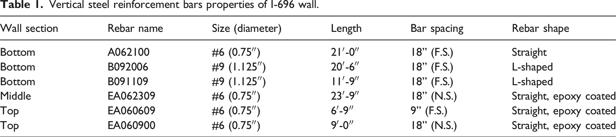
The construction of the wall panel occurred in multiple stages with the footing cast first. Next, the primary retaining wall was cast as two sections with a cold joint between the sections. The primary wall has a total height of 18.6 ft (5.7 m) with a tapered section with a 3 ft (0.91 m) bottom thickness to 1.8 ft (0.55 m) top thickness. The last stage of construction was the placement of a 9.9 ft (3.0 m) tall parapet wall with a constant thickness of 1.5 ft (0.46 m). At the street level, the far-side (F.S.) surface of the parapet wall is bricked to enhance the wall aesthetic along Eleven Mile Road. Both horizontal and vertical steel reinforcement bars were used in the wall construction as shown in Figure 2(c).

To accommodate the high tensile response of the wall, the vertical steel rebar is denser on the F.S. of the wall to accommodate the high levels of tensile flexural strain. The F.S. reinforcement is also continuous through the height of the wall ensuring full compatibility of the wall segments. Due to the thicker section and denser steel reinforcement, the lower portion of the wall has a much higher flexural rigidity to accommodate the higher flexural moments induced by the lateral earth pressures on the F.S. side of the wall. In contrast, the top parapet wall is thinner and more lightly reinforced due to low flexural demands placed on this portion of the wall. The concrete cover over the wall reinforcement is 3 in (7.6 cm) in most locations of the F.S. and N.S. of the wall; however, the reinforcement bar cover is 3.625 in (9.2 cm) on the N.S. face of the lower wall portion. The steel reinforcement used is summarized in Table 1.

Table 1.

Vertical steel reinforcement bars properties of I-696 wall.

Wall section	Rebar name	Size (diameter)	Length	Bar spacing	Rebar shape
Bottom	A062100	#6 (0.75″)	21′-0″	18” (F.S.)	Straight
Bottom	B092006	#9 (1.125″)	20′-6″	18” (F.S.)	L-shaped
Bottom	B091109	#9 (1.125″)	11′-9″	18” (F.S.)	L-shaped
Middle	EA062309	#6 (0.75″)	23′-9″	18” (N.S.)	Straight, epoxy coated
Top	EA060609	#6 (0.75″)	6′-9″	9” (F.S.)	Straight, epoxy coated
Top	EA060900	#6 (0.75″)	9′-0″	18” (N.S.)	Straight, epoxy coated

I-696 wireless monitoring system

A wireless structural monitoring system is selected for long-term monitoring of the I-696 retaining wall segment (Admassu et al., 2019). Since their inception in the mid-1990s (Straser et al., 1998), wireless structural monitoring systems have matured and today are a proven cost-effective solution for long-term monitoring of civil engineering structures including bridges (Pakzad et al., 2008), buildings (Kurata et al., 2005), and wind turbines (Swartz et al., 2010). The wireless monitoring system is designed using the Urbano wireless sensor node (Flanigan and Lynch, 2018) which is architecturally based on the Narada wireless node (Swartz et al., 2005) that has been widely used for long-term monitoring of bridges (Flanigan et al., 2020; Hou et al., 2020; Kurata et al., 2013; Zhang et al., 2017). Urbano was designed to operate on less battery energy than Narada and relies on the use of 4G cellular modem (Nimbelink Skywire) to transmit its data to the Internet. Cellular communications are attractive because they eliminate the need for on-site base stations while offering precise time synchronization of the node based on the GPS clock maintained by the cellular provider at the cell tower. The cellular modem consumes 616 mA (referenced at 3.3 V) when transmitting, 48 mA when idle, and 8.6 mA when in low-power mode. The seemingly high-current associated with transmitting is offset by the high data rates supported by the radio including a 5 Mbps upload rate. When the radio is needed, Urbano is designed to turn the radio on for bursting out data and then placing it back into sleep mode to minimize battery energy consumption when not transmitting (Admassu et al., 2022). At the core of Urbano is an 8-bit microcontroller (Atmel ATmega2561) clocked at 8 MHz and powered by a 3.3 V power supply. The microcontroller has 256 kB of flash memory for program storage and 8 kB of SRAM for data storage. Volatile memory is further expanded with an additional 512 kB of SRAM (Cypress CY62148EV30) included in the node design. The 8-bit microcontroller includes a multi-channel 10-bit analog-to-digital converter (ADC) capable of a maximum sample rate of 200 kHz. The ATmega2561 alone draws 7.3 mA when active, but 4.5 µA when in power-save mode.

To monitor the behavior of the I-696 wall segment, three sensing transducer types are selected and integrated with Urbano: tiltmeter to measure wall tilt, long-gage strain gage to measure thermal and flexural strain, and thermistor to measure wall temperatures. These three transducers are selected to offer insight into different aspects of the wall behavior in its loading environment. To measure tilt, a 9-axis absolute orientation sensor (Bosch BNO055) well suited for static tilt measurements is adopted to measure the pitch, roll and yaw of the wall. The internal BNO055 accelerometer has an acceleration measurement range of 2g with a resolution of 1 mg (Bosch, 2016). The three static accelerations measured by the BNO055 sensor are used to estimate the tilt of the sensor with a resolution of 0.01°. The BNO055 sensor is interfaced to the wireless node using a serial interface with the Urbano microcontroller. The microcontroller is programmed to query the three static acceleration measurements of the sensor: A_x, A_y, A_z with x, y, and z directions corresponding to vertical along the wall face (in the direction of gravity), orthogonal to the wall plane, and horizontal along the wall face, respectively (as shown in Figure 4(a)). The tilt of the wall along the z-direction can be estimated in radians using the x- and y-accelerations:

θ_{z} = \tan^{- 1} (\frac{A_{x}}{A_{y}})

(1)

An additional feature of the BNO055 is that it includes temperature compensation providing thermally stable measurements between −40°C (−40°F) and 125°C (257°F). To improve the accuracy of the tilt measurement, Urbano is programmed to read 100 consecutive acceleration measurements at 100 Hz with the collected measurements averaged before tilt, θ_z, is autonomously calculated by the node using equation (1).

To create a strain sensor to measure the thermal and flexural strain response of the wall, four 350 Ω metal foil strain gages (Omega KFH-6-350-C1-11L1M2R) are bonded to a 1 ft (0.30 m) long, 2 in wide (5.1 cm) and 0.25 in (0.64 cm) thick aluminum plate in a cross configuration (as shown in Figure 3(a)). Two strain gages aligned with the main axis of the aluminum plate (with resistances denoted as R_F1 and R_F4) are interfaced to opposite sides of a Wheatstone bridge while the other two gages are oriented orthogonal to the main axis (with resistances denoted as R_F2 and R_F3) are interfaced to the other two opposite sides of the Wheatstone bridge (Figure 3(b)). This configuration enhances the sensitivity of the strain response along the length of the plate while using the two gages orthogonal to the plate’s longitudinal axis to thermally compensate the bridge circuit. The gages in the Wheatstone bridge are powered using a 3.3 V source (V_in) with the bridge output voltage (V_out) fed into a standard instrumentation amplifier (Analog Devices AD623) whose internal gain is set to 1000 resulting in V_strain (=1000*V_out). The amplified output of the amplifier, V_strain, is connected to the Urbano 10-bit ADC for data collection. This full bridge setup allows longitudinal strain in the plate, ε, to be calculated as: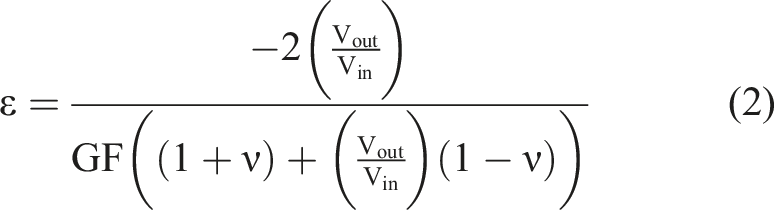

ε = \frac{- 2 (\frac{V_{out}}{V_{in}})}{GF ((1 + ν) + (\frac{V_{out}}{V_{in}}) (1 - ν))}

(2)

where GF is the gage factor of the metal foil gages (GF = 2.05) and ν is the Poisson ratio of the aluminum plate (ν = 0.33). Prior to deployment of the aluminum plate, a conformal polymeric coating is applied to the gages and their lead wires to fully seal them from the harsh operational environment anticipated.

The last sensor used to monitor the I-696 retaining wall panel is a standard, waterproof thermistor (TDK Group B57020M2). The thermistor is interfaced to a voltage divider circuit to convert resistance to a voltage that is read by the Urbano 10-bit ADC. The Urbano node is programmed to estimate the strain and wall temperature based on the voltages read from the signal conditioning circuits used for the aluminum plate strain sensors and thermistor.

Figure 3.

Long-gage strain sensor: (a) long-gage aluminum plate with four active metal foil strain gages attached; (b) full-bridge circuit interfaced to Urbano.

The Urbano wireless sensor node is packaged in a water-tight NEMA-rated enclosure prior to deployment on the I-696 retaining wall systems. As shown in Figure 4(b), inside each enclosure is an Urbano node, signal conditioning circuits, solar charge controller, and a 12V (2.9 A-hr) sealed rechargeable lead acid battery (Powersonic PS-1229). The enclosures also included the Bosch BNO055 bonded to the enclosure’s bottom surface shielding it from direct sunlight. The node enclosure is attached to the wall surface using four threaded bolts anchored into the wall as shown in Figure 4(a). The aluminum plate strain sensors and thermistors are attached to the wall with wires from these sensors fed into the enclosures through watertight glands and attached to the Urbano node. The thermistor is epoxied to the wall surface while the aluminum plate strain sensor is attached using two threaded bolts anchored into the wall. The thermistor and the strain gages on the strain sensing plate are both covered with a waterproof epoxy-like coating to ensure rain and sunlight do not affect the measurements. Each node is powered by a 12V (10 W) solar panel (Acopower HY010-12M) attached to a light pole above the retaining wall (Figure 4(c)).

Figure 4.

(a) Urbano wireless sensor units 2 and 3 in Figure 2(a) and an aluminum plate strain sensor; (b) interior view of the NEMA enclosure showing Urbano node, solar charge controller, BNO055 sensor, and lead acid rechargeable battery; (c) solar panels used to power nodes.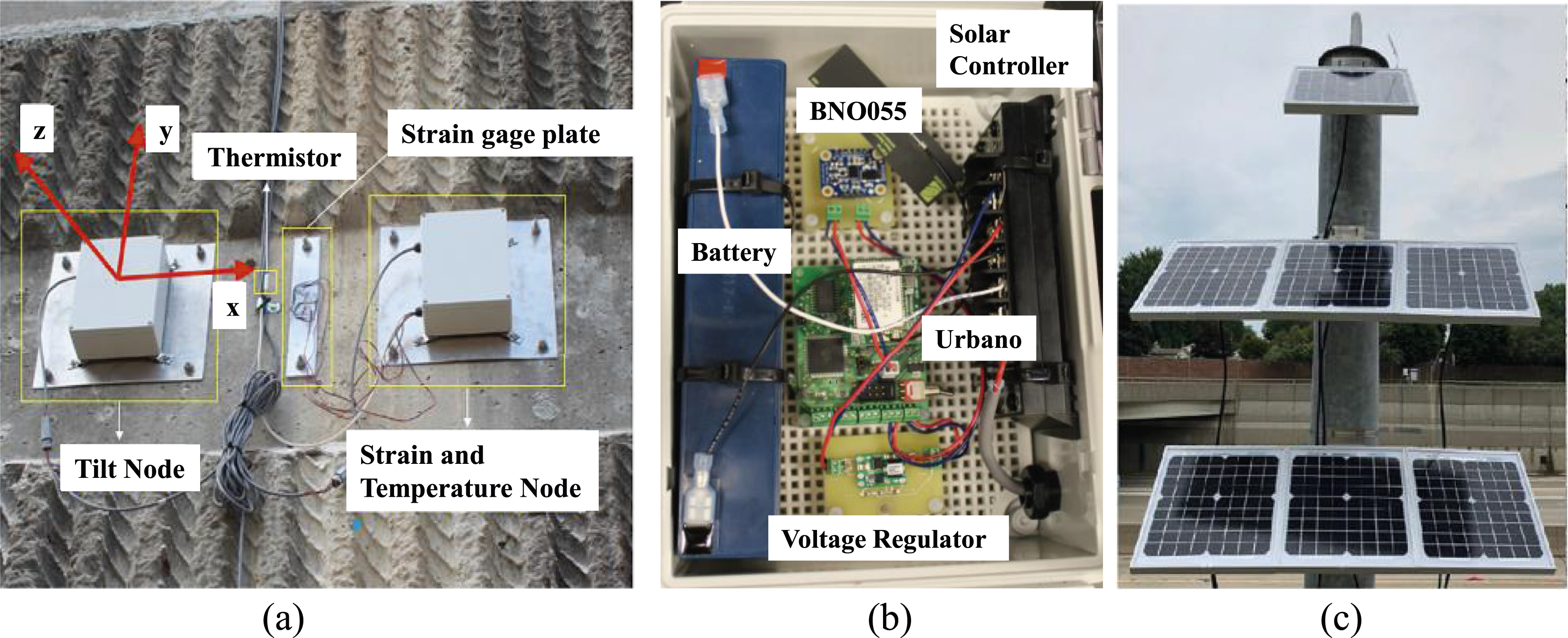

A total of four Urbano wireless sensor nodes are deployed along the center line of the I-696 retaining wall segment on August 25, 2018, during a warm and dry day; the locations of the four nodes are denoted in Figure 2(a). To measure wall tilt at the top (θ_top) and mid-height (θ_mid), Node 1 is installed at 24 ft (7.3 m) above grade and Node 2 at 13.5 ft (4.1 m) above grade, respectively. To measure wall strain at mid-height (ε_mid) and bottom (ε_bot), Node 3 is installed 13.5 ft (4.1 m) above grade while Node 4 is installed at 3.5 ft (1.1 m) above grade, respectively. A thermistor is interfaced to both Nodes 3 and 4 to measure the surface wall temperature (T_mid and T_bot, respectively) in addition to strain. The Urbano wireless nodes are designed to operate on a schedule with each node programmed to collect data every hour; when not sensing, the nodes remain in a low-power state to preserve battery energy. After data is sampled by each node, the nodes are programmed to communicate data to a cloud server using the cellular modem integrated with each node. In this study, the I-696 wall is monitored from August 2018 to February 2020.

Methodology: Analytical framework for reliability assessment

Model of wall behavior to extract lateral loads

The primary objective of the analytical framework is to process the measured response of the instrumented retaining wall to estimate the system reliability using user-defined limit states. A challenge for this task is the complex nature of the wall behavior. Specifically, the observed wall behavior will primarily be in response to both thermal variations and lateral earth pressures. The monitoring system is designed to produce response data that would allow the wall strain response to thermal and lateral earth pressure loads to be disaggregated as separate response components. Specifically, the thermal and flexural strain components will be denoted as ε_temp and ε_flex, respectively, with total strain, ε, the sum of the two components: ε = ε_temp + ε_flex. Absolute strain cannot be measured using the instrumentation described previously because there are residual strains inherent in the wall system at the time of the installation of the strain sensors. Hence, measured changes in strain, Δε, as referenced from the start of the monitoring campaign and are associated with changes in wall temperature, ΔT, in addition to changes in the lateral earth pressures on the far-side of the wall over the period of monitoring:

∆ ε = {∆ ε}_{t e m p} + {∆ ε}_{f l e x}

(3)

Thermal strain changes, ${∆ ε}_{t e m p}$ , are a result of the change in the wall temperature, ΔT, as measured by the thermistors and are assumed to be uniform across the cross-section of the wall. It is recognized that the temperature of the wall is likely to have a gradient across its thickness but due to the lack of measurement of the wall backside temperature, the assumption of a uniform temperature distribution is reasonable.

In theory, the relationship between thermal strain change and temperature is defined as:

{∆ ε}_{t e m p} = α_{e f f} Δ T

(4)

where α_eff is defined as the effective thermal expansion coefficient of the wall system. Given that the thermal behavior of the RC wall, namely α_eff, is not known a priori, equation (4) cannot be used to define

{∆ ε}_{t e m p}

. An alternative approach is to determine

{∆ ε}_{f l e x}

using the tilt measurements allowing the flexural component to be subtracted from measured changes in strain, Δε.

Wall tilt measurements, $θ_{m e a s} = {[\begin{array}{l} θ_{t o p} & θ_{m i d} \end{array}]}^{T}$ , are primarily in response to the lateral earth pressures that exist behind the wall as shown in Figure 5. Changes in lateral earth pressures will result from changes in the surcharge load, q, at the top of the wall and the level of hydraulic pressure applied to the wall based on the height of the groundwater table, h_sat. Soil properties such as soil friction angle, ϕ, bulk density, γ_b, and submerged density, γ′, are assumed to remain unchanged during the monitoring period. A mechanical model of the flexural response of the wall is proposed to use the two absolute tilt measurements, θ_top and θ_mid, to estimate the height of the water table, h_sat, and surcharge load, q. Such a model would allow each tilt measurement vector, $θ_{m e a s}$ , to be converted to an estimated loading profile defined by q and h_sat. In using a mechanical model of the wall in this manner, an estimation of the lateral earth pressures is obtained from which the same model can be used to define $ε_{f l e x}$ at any wall location. Using equation (3), changes in flexural strain, ${∆ ε}_{f l e x}$ , over the monitoring period can then be used to estimate changes in thermal strain, ${∆ ε}_{t e m p}$ , based on changes in the measured strain, $∆ ε$ .

Figure 5.

Active lateral earth pressures behind the monitored wall due to surface surcharge loading, hydrostatic pressure, and backfill pressure.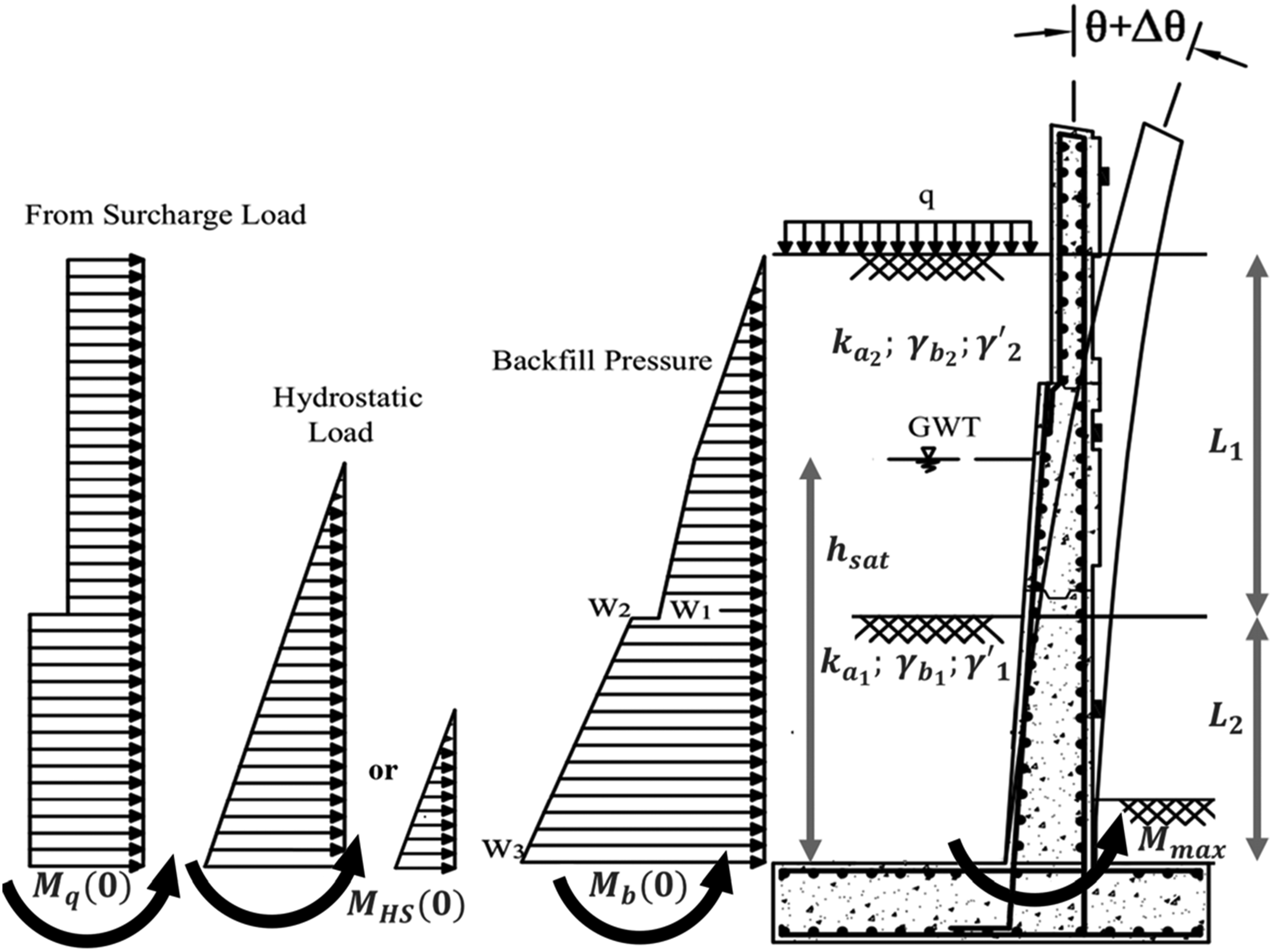

To develop a simple mechanical model of the retaining wall, it is modeled as a Euler–Bernoulli beam model with the interaction between adjacent wall panels ignored to ensure model simplicity. The beam is assumed to be in static equilibrium governed by the moment balance:

E_{e} (x) I_{c r} (x) (\frac{d^{2} y (x)}{d x^{2}}) = E_{e} (x) I_{c r} (x) (\frac{d θ (x)}{d x}) = M (x)

(5)

where

M (x)

is the flexural moment induced by the backfill,

y (x)

is the displacement of the wall, and

θ (x)

is the wall tilt, with equilibrium defined at the wall height, x. The effective modulus of the composite RC cross-section is defined as E_e and the moment of inertia of the section is defined based on the assumption of a cracked section,

I_{c r}

(which assumes the concrete carries no tensile load on the far-side of the wall). The cracked section assumption is valid given the age of the wall, the large flexural loads present, and visual evidence of flexural cracking in previously excavated retaining walls of the same vintage in southeast Michigan (MDOT, 2013). To accommodate the tapered vertical profile of the wall and varying reinforcement detailing through the wall height, the beam model is discretized into k segments each with a horizontal height of

δ h

= 1 in (2.54 cm). This element height (i.e.,

δ h

= 1 in.) for the discrete element analysis was selected after a sensitivity analysis was performed balancing accuracy with computing time. While a larger element height could have been used, the ability to accurately capture the geometric details of the wall backside tapering and changes in reinforcement bar layouts at different heights at the expense of extra computation time was favored.

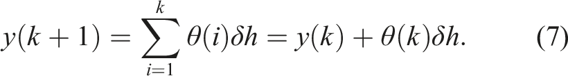
For a given loading profile, q and h_sat, the vertical profile of lateral earth pressures is established and the moment distribution, M(x), calculated by standard equilibrium principles. The wall rotations, $θ (x)$ , and deflections, $y (x),$ are then calculated using a discretized approach to analysis starting from the base element whose index is i = 1 to the top of the wall whose index is i = k:

θ (k + 1) = \sum_{i = 1}^{k} \frac{M (i)}{E_{e} I_{c r} (i)} = θ (k) + δ h \frac{M (k)}{E_{e} I_{c r} (k)}

(6)

y (k + 1) = \sum_{i = 1}^{k} θ (i) δ h = y (k) + θ (k) δ h .

(7)

Given the age of the retaining wall system, the material properties of the concrete need to account for age, especially in the selection of the concrete modulus of elasticity. The effective modulus of the concrete is determined based on the documented 28-days compressive strength of the concrete (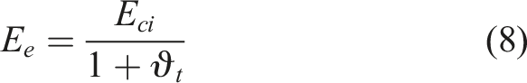 $f_{c}^{'}$ = 4000 psi (27.6 MPa)) at the time of construction with creep and shrinkage considered. The effective modulus, $E_{e}$ , is based on the initial modulus, $E_{c i} = 57, 000 \sqrt{f_{c}^{'}}$ (in psi) and the creep coefficient, $ϑ_{t}$ , with t specified in days (ACI, 1997):

E_{e} = \frac{E_{c i}}{1 + ϑ_{t}}

(8)

ϑ_{t} = 2.35 * \frac{t^{0.6}}{1 + t^{0.6}} .

(9)

Given the age of the wall (33 years), the effective modulus, $E_{e}$ , was determined to be 1.1 × 10⁶ psi (7.6 GPa) based on equations (8) and (9). The elastic modulus of steel is assumed to be $E_{s} = 29.0 x 10^{6} psi (210 GPa)$ .

With respect to the soil backfill, the soil boring elevation drawings document the backfill as a two-layer system with a 13.9 ft (4.2 m) thick layer of medium compacted sand on top of a 9.6 ft (2.9 m) thick layer of medium compacted gray silt and fine sand. In the absence of site-specific information, based on (Coduto, 2001; NAVFAC, 1986), the medium compacted sand is assumed to have a bulk density of γ_b2 = 119.2 lb/ft³ (1909.9 kg/m³) and submerged density of γ₂' = 65.7 lb/ft³ (1051.8 kg/m³) while the medium compacted gray silt and fine sand layer is assumed to have a bulk density of γ_b1 = 126.1 lb/ft³ (2020.6 kg/m³) and submerged density of γ₁' = 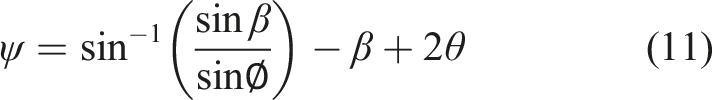72.6 lb/ft³ (1162.6 kg/m³). Rankine’s theory is used to determine the pressures on the far-side of the wall, a methodology also favored by state transportation agencies including AASHTO and FHWA. The generalized form of Rankine’s earth pressure coefficient, k_a, for each layer is (Chu, 1991):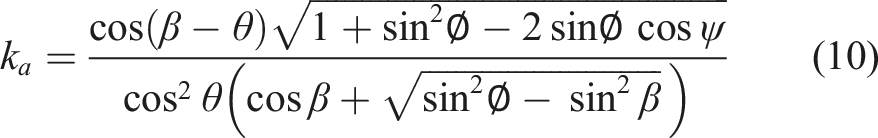

k_{a} = \frac{\cos (β - θ) \sqrt{{1 + \sin}^{2} \emptyset - 2 \sin \emptyset \cos ψ}}{\cos^{2} θ (\cos β + \sqrt{\sin^{2} \emptyset - \sin^{2} β})}

(10)

ψ = \sin^{- 1} (\frac{\sin β}{\sin \emptyset}) - β + 2 θ

(11)

where β is the slope of the top surface of the backfill relative to the horizon (in this case β = 0°), ϕ is the internal soil friction angle, and

θ

is the slope of the wall F.S. surface (relative to vertical). Typical angles of internal soil friction were acquired from (Koloski et al., 1989): sand with medium compaction, ϕ = 33°, and sandy silt with medium compaction, ϕ = 29°. The angle of the back surface of the instrumented wall,

θ

, is computed as 3.6° based on the structural drawings. Using equations (10) and (11), the active earth pressure coefficients are computed as k_a2 = 0.30 and k_a1 = 0.35 for the upper and lower soil layers, respectively.

To simplify the analysis, permutations of q and $h_{s a t}$ are varied with the model to estimate the top and mid-height wall rotations: $θ_{m o d e l}$ . A total of 17 increments of surcharge pressure were considered between 0 and 1.74 psi (12.0 kPa); similarly, 282 increments of water saturation levels were considered between 0 and 282 in (7.16 m). A look-up table is created for every permutation of q and $h_{s a t}$ . For a given measurement of wall tilt, $θ_{m e a s}$ , the optimal load profile can be found by finding the table element that minimizes the difference between the measured and the model tilt,

{({q, h}_{s a t})}_{o p t} = \begin{array}{l} argmin \\ q, h_{s a t} \end{array} ‖ θ_{m e a s} - θ_{m o d e l} ‖

(12)

With the optimal load profile estimated, the flexural strain response, $ε_{f l e x},$ can be modeled anywhere in the wall cross-section. Using the initial flexural strain measurement at the start of the monitoring campaign, changes in flexural strain, ${∆ ε}_{f l e x}$ , at the points of strain measurement can be calculated so that change in thermal strain, ${∆ ε}_{t e m p}$ , can be extracted from changes in the measured strain, $∆ ε$ , by equation (3). It should be noted that this modeling approach is fully deterministic and assumes accurate estimation of the properties of the structural and backfill material properties. Measured changes in thermal strain, ${∆ ε}_{t e m p}$ , and wall temperature, $∆ T$ , can then be used to empirically estimate the effective thermal expansion coefficient, α_eff, by linear regression analysis. A summary of the algorithmic framework for load estimation and thermal strain extraction is shown in Figure 6.

Figure 6.

Load estimation and thermal strain extraction from measurement data.

Reliability methods for retaining wall performance assessment

At the core of quantitative risk assessment is a structural reliability assessment using monitoring data. Reliability assessments calculate the probability of exceeding a defined scalar limit state function, G( X ) where X is a vector of random variables, $X = {[X_{1}, X_{2}, \dots, X_{n}]}^{T}$ . The limit state function reflects the margin that exists between the system capacity, C, and demand, D: $G (X) = C - D$ . Various limit states can be formulated based on strength or serviceability considerations.

The probability of failure, $P_{f}$ , is defined as the probability of X existing in the failure domain, $Ω$ :

P_{f} = \int_{Ω} f_{X} (X) d X where Ω \equiv G (X) \leq 0

(13)

When working within independent standard normal space, the reliability index,

β

, is defined as the minimum distance from the origin to where

G (X) = 0

. As a result,

P_{f}

and

β

are related by

P_{f} = Φ (- β)

where

Φ (\cdot)

is the standard normal cumulative distribution function. The probability of failure can be multiplied by the consequence of failure, C_$, to estimate the system risk: R =

P_{f} \times C_{$}

. The consequences can be described in the form of monetary costs including the cost of system repair, cost of damage to other physical assets, opportunity cost (such as the cost of road closures), and cost of human life lost. In this study, the analytical framework focuses on a reliability assessment using monitoring data and leaves the complete risk assessment to end users who have robustly defined the consequences of failure.

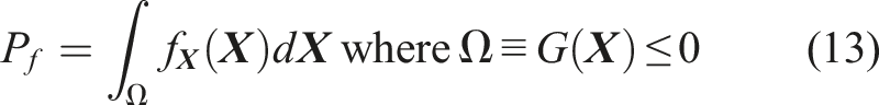
Reliability methods are integral to the design of earth retaining structures including retaining walls that are designed using load and resistance factor design (LRFD) codes such as those associated with AASHTO. Researchers have explored reliability methods to advance the design of retaining walls. For example, (Low, 2005) explored the use of the Hasofer–Lind reliability index and the first-order reliability method (FORM) to design retaining walls to target reliability index values. (Basheer and Najjar, 1996) developed a reliability framework to optimize the design of reinforcing ties used in the design of reinforced earth retaining walls. (Goh and Kulhawy, 2005) studied the use of neural networks to define nonlinear limit state functions that define unacceptable excessive ground deformations associated with braced retaining walls used in excavation projects. More recently, there has been research devoted to expanding the role of reliability from the design phase of a structure to that of asset management, especially of bridges. For example, (Zonta et al., 2007) proposed a decision support system for bridge managers based on reliability methods using visual inspection ratings and associated data. The seminal study by (Frangopol et al., 2008) explored the inclusion of long-term strain data in estimating the reliability of bridge components based on the use of FORM to estimate the reliability index of an instrumented truss element. Similarly, (Flanigan et al., 2020) proposed the use of strain data to assess the reliability of fatigue-critical structural elements in a railroad truss bridge.

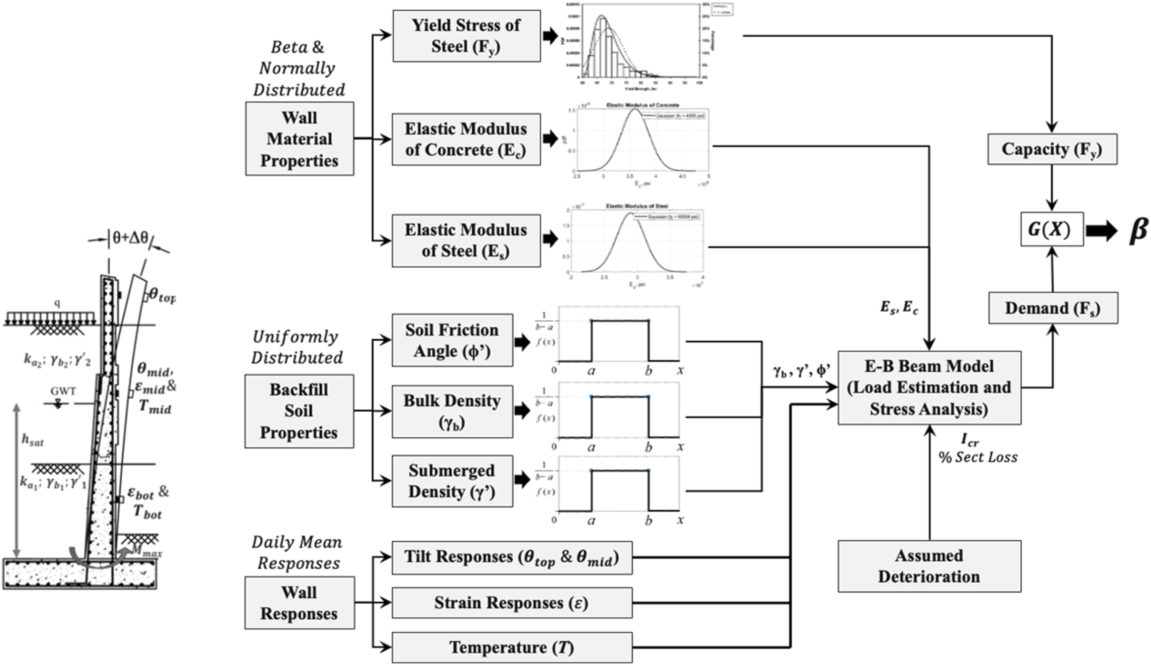
At the core of the reliability assessment method proposed herein (Figure 7) is the use of the Euler–Bernoulli beam model previously developed to determine the demand response, D, of the retaining wall to the observed lateral earth pressures and thermal loads estimated from the monitoring data. A Monte Carlo approach is taken to perform the reliability assessment given the computational simplicity of the Euler–Bernoulli beam model. First, for a given state of measurement $M = {[\begin{array}{l} \begin{array}{l} θ_{t o p} & θ_{m i d} \end{array} & \begin{array}{l} ε_{m i d} & \begin{array}{l} ε_{b o t} & T \end{array} \end{array} \end{array}]}^{T}$ , a reliability assessment is performed to estimate the reliability index, β_M, to a user-defined limit state function, G( X ). In each iteration of the Monte Carlo implementation, the material properties for the wall and soil are treated as random variables, X $= {[\begin{array}{l} \begin{array}{l} E_{c i} & E_{s} \end{array} & \begin{array}{l} ϕ & \begin{array}{l} γ_{b} & γ^{'} \end{array} \end{array} \end{array}]}^{T}$ sampled from assumed distributions. For a sampling of X , the measurements, M , are used to extract the loads q and h_sat using the same beam model method as proposed in the previous section. The load parameters are then applied to the beam model to determine the demand response of the wall, D. A statistical model of the system capacity, C, is sampled to determine if G( X ) < 0. For N iterations of the method, the number of times the limit state function is negative is counted, n, to determine the probability of failure: P_f = n/N. Finally, reliability index (β_M) is calculated as:

β_{M} = Φ^{- 1} (P_{f}) .

(14)

Figure 7.

Analytical framework of reliability analysis using probabilistic models for system properties.

A primary failure mechanism of cantilever retaining walls is the corrosion of the steel reinforcement at the base of the wall with lateral earth pressures producing an overturning moment, M_b(0), that exceeds the flexural capacity of the base cross-section. In the case of the retaining wall studied in this work, evidence of continuous water drainage at the base of the wall makes corrosion of the steel reinforcement a long-term concern. Hence, this study considers the limit state function as the difference in the demand response, $ε_{s}$ , in the tensile steel reinforcement at the base of the wall and its capacity as defined by its yield stress, F_y:

G (X) = F_{y} - ε_{s} \cdot E_{s} .

(15)

This is just one of many possible limit state function that the wall owner may want to consider; the reliability assessment framework is capable of accommodating other limit state functions. For each iteration of the Monte Carlo analysis, the strain in the steel reinforcement is calculated based on, $ε_{s, f l e x},$ using the lateral earth pressures estimated from the wall tilt measurements and changes in the thermal strain extracted from the strain data at the bottom of the wall ${∆ ε}_{b o t, t e m p}$ using equation (4).

With respect to the random variables, X , the elastic moduli of structural materials are well established to follow normal distributions. For concrete, the distribution of concrete elastic modulus is presented as Gaussian for different compressive strength grades in (Mokhtar et al., 2013), while it is presented likewise for structural steel in (Arrayago et al., 2020) and reinforcement bars by (Mirza and MacGregor, 1979). Hence, the elastic modulus of concrete, E_ci, is assumed to be normally distributed with mean $3.6 x 1 0^{6} psi (24.8 GPa)$ and standard deviation $0.25 x 1 0^{6} psi (1.74 GPa)$ with equation (8) used to determine the effective elastic modulus, E_e. The elastic modulus of steel, E_s, is also treated as normally distributed with mean $29.0 x 10^{6} psi (210 GPa)$ and standard deviation $1 x 10^{6} psi (210 GPa)$ . The probabilistic models used to define soil properties vary but are conservatively assumed to be uniformly distributed. The uniformly distributed bulk and submerged densities of the two soil types in this study are based on (NAVFAC, 1986). The medium compacted sand is conservatively assumed to have a bulk density with a significant variation from γ_b2 = 84.7 lb/ft³ (1462.3 kg/m³) to 136.5 lb/ft³ (2357.5 kg/m³) and submerged density that varies from γ₂' = 51.8 lb/ft³ (876.5 kg/m³) to 72.6 lb/ft³ (1227.1 kg/m³). The medium compacted gray silt and fine sand layer is assumed to have a bulk density that varies uniformly from γ_b1 = 88.1 lb/ft³ (1411.7 kg/m³) to 141.7 lb/ft³ (2269.7 kg/m³) and submerged density that varies from γ₁' = 53.6 lb/ft³ (858.1 kg/m³) to 79.5 lb/ft³ (1273.3 kg/m³). Typical angles of internal soil friction were acquired from (Koloski et al., 1989): sand with medium compaction uniformly distributed from ϕ = 30° to 35° while sandy silt with medium compaction uniformly varied from ϕ = 20° to 30°. The internal soil friction angles were used to estimate the Rankine’s earth pressure coefficient, k_a, by equation (10).

For the limit state function used in this study, a statistical distribution of F_y is assumed based on the comprehensive statistical modeling of steel reinforcement properties by (Bournonville et al., 2004). For the ASTM A615 Grade 60 steel reinforcement used at the base of the wall, a normal distribution is assumed. Based on (Bournonville et al., 2004), the mean yield strength of Grade 60 steel is 69 ksi (475 MPa) with a standard deviation between 4.3 ksi (29.6 kPa) and 5.0 ksi (34.5 kPa); this study selected 5.0 ksi (34.5 kPa) for the standard deviation.

Results

Long-term behavior of retaining wall

The cantilever retaining wall panel was monitored continuously from August 2018 to February 2020. Figure 8 provides a continuous time history of the measured wall tilts ( $θ_{t o p}$ and $θ_{m i d}$ ), strain ( $ε_{m i d}$ and $ε_{b o t}$ ), and wall temperature (T) for each day averaged over a 24-h period from 12:00 am to 11:59 pm. It should be noted that the strain measurements are the raw change in strain with each strain sensor zeroed at the first reading in August 2018. Overall, the wireless sensors that collect data from the retaining wall sensors work well during the entire measurement campaign with only the Urbano node measuring strain and temperature at the bottom of the wall failing in late July 2019. Intermittently, some of the sensors do not report their data resulting in some gaps in the measurement time histories shown in Figure 8. Also included in Figure 8 is a history of precipitation recorded by weather station KMISOUTH67 only 2 miles (3.2 km) away (Weather Underground, 2022); precipitation is an important environmental parameter that will influence h_sat.

Figure 8.

Daily mean responses of the I-696 retaining wall panel with daily mean precipitation added (August 2018 - February 2020).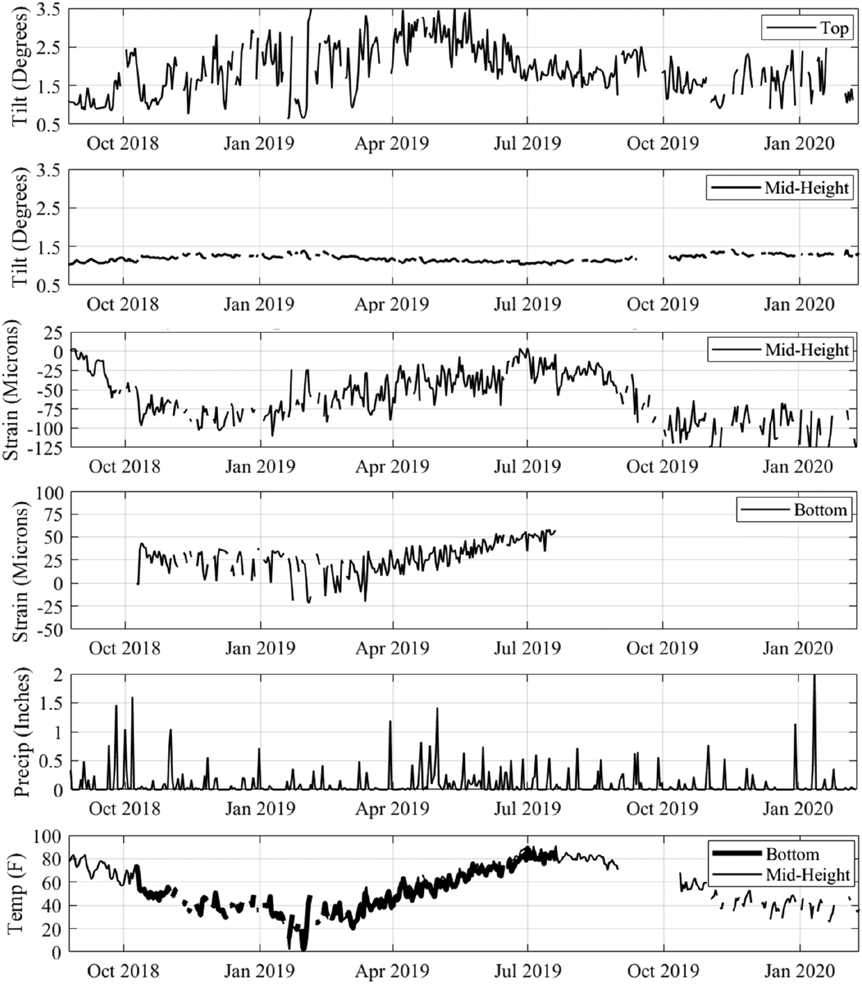

The gaps in data observed in the time history plots (i.e., wall responses in Figure 8, the plots of estimated tilt, surcharge load, and saturation level in Figure 13, and reliability indices in Figure 15) are attributed to two main factors. The first is that wireless sensor units can have low battery charges due to the slow rate of recharging the battery by the solar panels during cloudy or very cold days. If the battery charge is low, the cellular modem is kept off. Second, the cellular network signal in the wall location is sometimes not strong enough for the Urbano nodes to communicate to the 4G network necessary to transfer data to the cloud-based database. One solution is to use slightly larger batteries and solar panels; another is to buffer data in local memory to report to the database when the network signal is strong enough.

The tilt history of the top portion of the wall system demonstrates a greater variation in daily mean tilt as compared to the mid-height tilt. Specifically, the top tilt varies from 0.5 to 3.5° while the mid-height tilt has a much smaller variation between 1.0 and 1.45°. The top-level tilt sensor was installed upon the thin parapet wall just 2 ft (0.6 m) below the wall top (Figure 2(a)). The wide variation in tilt of the parapet wall was attributed to the fact that maximum rotations of the wall due to lateral earth pressures will be at the top of the wall. Also contributing is the lower flexural rigidity of the parapet wall due to a lower thickness and lighter steel reinforcement. During certain periods, repeated days of precipitation seem to influence the top wall tilt possibly due to the build-up of hydraulic pressure in the top stratum of soil. For example, continuous days of rain from late September 2018 into early October 2018 induce a noticeable upper tilt of the top portion of the wall (going from 1.0 to 2.5°); after the rain ceases, the wall returns to 1.0°. Comparatively, the daily mean tilt of the lower portion of the wall is less sensitive to precipitation with little variations in daily mean wall tilts during periods of rain. This may be attributed to the high flexural rigidity of the wall; it may also be explained by the lack of variation in the hydrostatic pressures in the lower soil stratum behind the wall.

From late November 2018 to January 2019, the top tilt has a high level of day-to-day variation as the mean tilt increases slowly. It is also noted that the wall’s daily mean top tilt dramatically varies from mid-January 2019 to mid-February 2019 when the wall temperature is near or below freezing (32°F (0°C)). In the last few days of January 2019, the wall reaches a temperature of 0°F and a few days later a temperature of 42°F; during this period, the daily mean top wall tilt varies from 0.5 to 3.5° suggesting freezing of the backfill soil may be adding additional lateral earth pressures. By May 2019, the wall reaches a maximum daily mean top tilt of 3.5°. After May 2019, the tilt at the top of the wall has less day-to-day variation and the mean trend-line decreases to about 1.5° by July 2019. It is hypothesized that the daily mean top wall tilt trend-line slowly increases from November to May due to lowering ambient temperatures and their effects on the backfill soil resulting in greater lateral earth pressures. Comparing the daily mean top tilt trendline with the wall temperature time history, the two appear to be correlated with a 30 to 45 days lag; this may be attributed to thermal inertia of the backfill.

The daily mean strain responses at the wall mid-height and bottom capture changes in strain of the wall near-side; as previously mentioned, the absolute state of strain is unknown with measured strain always being relative to the start of monitoring in August 2018. Taking compressive strain to be of a negative magnitude, the daily mean wall strain histories exhibited a trend correlated to the wall temperature. The mid-height strain varied 125 με over the 15 months while the bottom strain varied only 75 με.

The causality between environmental parameters and the wall behavior are studied using response scatter plots with linear regressed behavioral models fit. Plotted in Figure 9 are scatter plots of lower wall responses (i.e., bottom strain, ${∆ ε}_{b o t}$ , mid-height strain, ${∆ ε}_{m i d}$ , and mid-height tilt, $θ_{m i d}$ ) as a function of measured wall temperature, T. As shown, a linear relationship exists between these two measurands. Using linear regression to model the relationship, it is evident that the mid-height tilt of the lower portion of the wall varies roughly 0.004° per degree F of wall temperature with a coefficient of determination (R²) of 0.47. The greatest mid-height tilt is experienced during the colder months with a maximum tilt of 1.4° when the wall temperature is 0°F. Similarly, the wall strain at the bottom and mid-height is dependent on temperature. Based on linear regression, the mid-height and bottom strain varies 0.92 με and 0.45 με per degree F, respectively. The coefficient of determination for the mid-height strain as a function of temperature suggests stronger linearity (R² = 0.51) than that of the bottom strain (R² = 0.11).

Figure 9.

Thermal behavior of the monitored retaining wall: (a) mid-height tilt, (b) mid-height strain, and (c) bottom strain (August 2018 – February 2020).

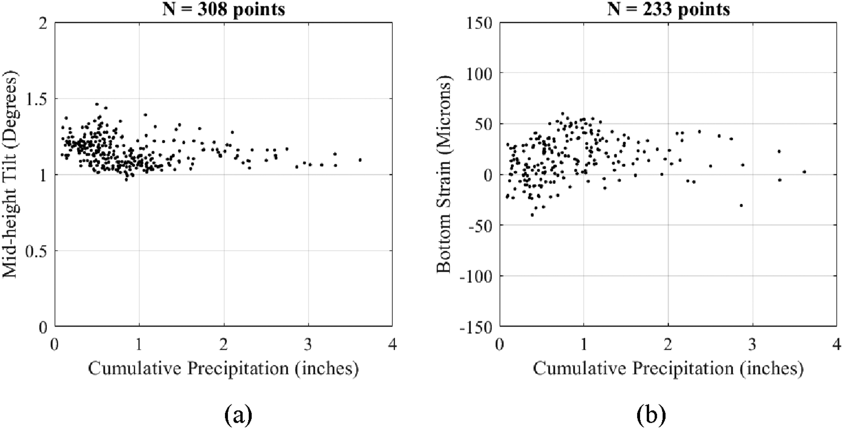
While the top tilt exhibits sensitivity to precipitation, the lower portion of the retaining wall is relatively insensitive to precipitation supporting the hypothesis that the lower portions of the wall backfill are normally saturated. Recall, this hypothesis was supported by visual observation of steady weeping in the wall panels in their lower sections, even during the dry summer months. As shown in Figure 10, the mid-height tilt and bottom strain of the wall panel are plotted as a function of cumulative precipitation. Cumulative precipitation is intended to model the time it takes for rainwater to permeate the soil and develop sustained hydrostatic pressure in the wall backfill. After periods of no precipitation, the cumulative precipitation model also assumes drying of the soil resulting in the alleviation of hydrostatic pressure. Here, it is assumed the cumulative rain, CR, is:

C R = \sum_{j = 0}^{i - 1} \frac{j}{i} D R (j) + \sum_{j = i}^{t} e^{α (i - j)} D R (j)

(16)

where DR is a daily time series of precipitation (in inches) with j serving as an index that begins at 0 and marches backward (e.g. 3 days prior is j = 3), i is a constant that reflects the tracking horizon (in days), t is a constant that reflects the time it takes (in days) for the soil to become unsaturated following saturation, and

α

is a time constant on the tail portion of the weighted sum. Using the wall top tilt and precipitation measurements collected during a period of heavy precipitation (e.g., late September 2018 into early October 2018), the cumulative rain function is empirically fit to find i = 3 days, t = 18 days and

α

= 0.1. As shown in Figure 10, the mid-height tilt and bottom strain of the wall panel are insensitive to cumulative rain, reinforcing the hypothesis of a saturated backfill.

Figure 10.

Precipitation induced response of the I-696 retaining wall: (a) mid-height tilt and (b) bottom strain (August 2018 – February 2020).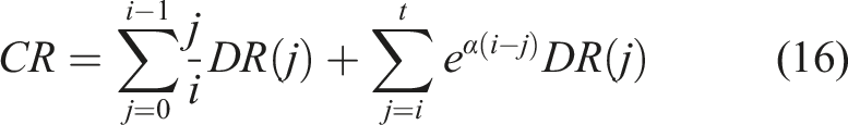

The behavior of the top portion of the wall panel, especially the parapet portion of the wall system, is observed to be sensitive to cumulative precipitation in the non-winter months while sensitive to temperature in the winter when there is less precipitation in the form of rain. Figure 11 plots the wall top tilt as a function of precipitation from August 25 to November 30, 2018 and April 1 to October 11, 2019 revealing a relatively linear relationship between top tilt and cumulative precipitation during the non-winter observation period. The figure also plots the top wall tilt as a function of wall temperature in the winter (January 1 to March 30, 2019) revealing a fairly strong (R² = 0.66) linear relationship of 0.05° per °F due to thermal expansion of the soil applying backfill lateral pressure.

Figure 11.

Tilt of wall top as a function of: (a) cumulative precipitation (8/25/18-11/30/18), (b) temperature (1/1/19-3/30/19), (c) cumulative precipitation (4/1/19-10/11/19).

Load modeling on the retaining wall

To check the measured tilts, a theoretical analysis with the Euler-Bernoulli beam model is performed to ascertain the theoretical smallest and largest tilt profiles using the mean properties of the random variables, X . Three lateral pressure profiles are explored on the I-696 wall panel: backfill lateral earth pressure, hydrostatic pressure, and surface surcharge pressure. The maximum lateral load on the wall is when all three lateral pressures act on the wall, simultaneously. The dry/moist backfill earth pressures remain constant while the hydrostatic and surcharge pressures correlate to h_sat and q, respectively. The maximum hydrostatic pressure occurs when h_sat is at the surface of the backfill (h_sat = 23.5 ft (7.2 m)). Similarly, a maximum surcharge pressure of q = 1.7 psi (11.7 kPa) is considered on the top surface of the backfill resulting in a uniformly distributed lateral earth pressure on the wall ( ${w = k}_{a} q$ ). This surface surcharge is conservatively obtained from the load assumptions used to design retaining walls (FHWA, 2009). Using the Euler-Bernoulli beam model (equations (6) and (7)), the wall deflection, y, is modeled for the best case (no surcharge or hydrostatic pressure) and worst case (q = 1.7 psi (11.7 kPa) and h_sat = 23.5 ft (7.2 m)) scenarios as shown in Figure 12.

Figure 12.

Deflected shapes of the cantilever wall under theoretical and actual conditions.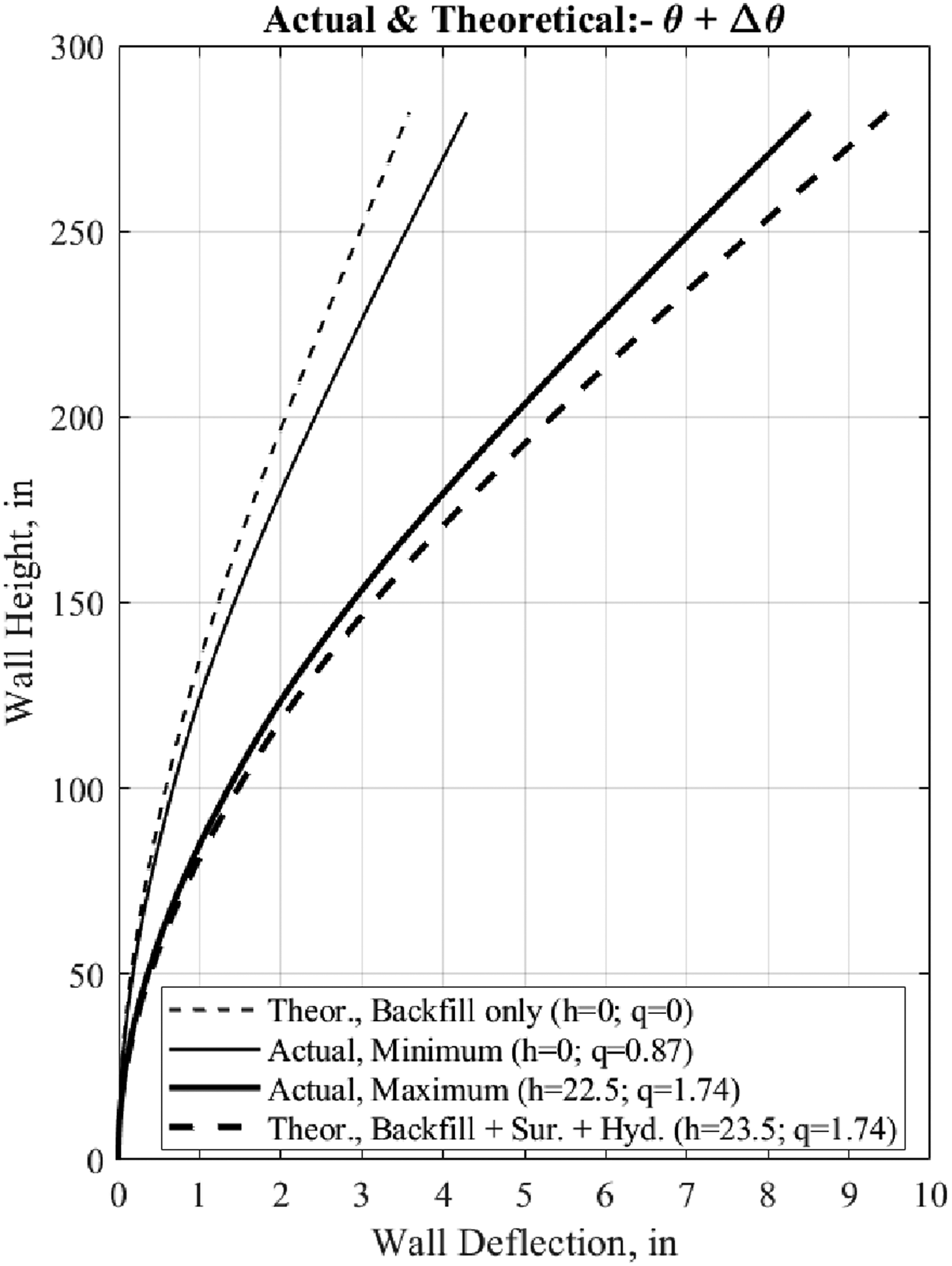

The Euler-Bernoulli beam model is also used to estimate the surcharge pressure, q, and level of groundwater table, h_sat from the top and mid-height tilts ( $θ_{t o p}$ and $θ_{m i d}$ ) based on the algorithmic framework presented in Figure 6. The estimated load parameters are shown in Figure 13 over the monitoring period. The estimated loading parameters can then be used in the model to calculate the deflected shape of the wall. Considering all measurements from the 18 months of monitoring, the least and greatest deflected shapes of the wall are found. On January 21, 2019, the measured tilts result in the least deflection based on a surcharge of q = 0.87 psi (6 kPa) and groundwater table height of h_sat = 0 ft (0 m). The maximum deflection occurs on April 10, 2019, with an optimal surcharge of q = 1.7 psi (11.7 kPa) and groundwater table height of h_sat = 22.5 ft (6.9 m). Both deflected wall profiles are presented in Figure 12. Estimating the deflected shapes of the wall can aid in understanding the seasonal variations observed in the data, especially the wall responses to hydrostatic pressures associated with precipitation.

Figure 13.

Daily mean response of tilt and estimation of surcharge load, q, and water saturation level, h_sat, based on I-696 retaining wall tilt measurements over 1 year of monitoring. Three states of steel section loss of the tensile reinforcement considered: 0, 10 and 20%.

With load parameters extracted for each daily wall response, the flexural strain, $ε_{f l e x}$ , is found for each load case at the bottom strain sensor location. Given the estimate of $ε_{f l e x}$ at the point of the bottom wall strain measurement, the change in strain due to flexure, ${∆ ε}_{f l e x}$ , relative to the start of the measurement of strain is calculated. Using equation (3), the change in thermal strain, ${∆ ε}_{t e m p}$ , is found by subtracting ${∆ ε}_{f l e x}$ from ${∆ ε}_{b o t}$ . Changes in ${∆ ε}_{t e m p}$ between sequential days is calculated and plotted based on the change in daily temperatures, $∆ T$ , as shown in Figure 14. The thermal expansion coefficient, α_eff, obtained was 1.89 με/°F which is close to those documented in the literature (i.e., 3 to 6 με/°F) for reinforced concrete (Berwanger and Sarkar, 1976).

Figure 14.

Scatter plot showing thermal strain response versus temperature change.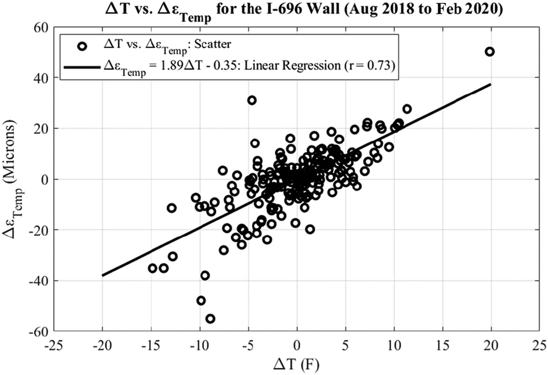

Reliability and risk analysis

The reliability analysis summarized in Figure 7 is applied to the mean response, $\bar{M}$ , calculated for each day of the measurement campaign using the limit state function of equation (15) applied at the tensile steel reinforcement at the base of the wall. Continuous drainage at the base of the I-696 retaining wall base suggests the lower portions of the wall backfill are saturated with water. With the cantilever wall experiencing tension on the wall backside, flexural cracks on the wall backside may expose the steel rebar to water. The steel rebar on the wall backside is standard steel (i.e., not epoxy coated) and has a 3″ cover (Figure 2). For the cantilever retaining wall monitored in this study, the steel rebar is suspected of having some form of corrosion and possible section loss, thereby reducing the flexural capacity of the wall. Failures of retaining walls of similar age and design due to the corrosion of steel components have been observed in the past in the region in which this wall is located. For example, panels of the M-10 retaining wall system in Detroit failed due to corrosion of tieback rods linking a section of the wall system to their caisson elements (MDOT, 2013). The challenge with retaining walls is that it is nearly impossible to assess if reinforcement bar corrosion is occurring without excavating the backfill. Should the backfill be excavated, several approaches are available for measuring the degree of corrosion including half-cell potential measurements and electro-impedance spectroscopy (Elsener et al., 2003). These methods were not practical for the operational cantilever retaining wall studied in this work.

The work of (Andrade and Alonso, 1996) is used to estimate the possible level of corrosion expected for a 33-year-old retaining wall with a moderate corrosion rate. If it is conservatively assumed that carbonation and chloride ingress occurred on the first day of construction and a moderate corrosion rate (e.g., 0.5 $μ$ A/cm²) exists, a section loss of 3% in the buried steel rebar is estimated. In this paper, three states of buried vertical steel reinforcement on the tensile side of the wall are assumed given the uncertainty associated with the degree of corrosivity of the operational environment: 0, 10 and 20 % section loss of the vertical steel rebar. The reliability, $β_{\bar{M}}$ , of the retaining wall panel is calculated for these three corrosion states. In the execution of the reliability analysis, the section loss is incorporated into the Euler-Bernoulli beam model of the retaining wall.

To perform a reliability analysis for each day of measurement, the Monte Carlo strategy samples the random variables of the model for a given level of assumed steel reinforcement corrosion (e.g., 0, 10, or 20%). The beam model is formed including the calculation of the neutral axis location, 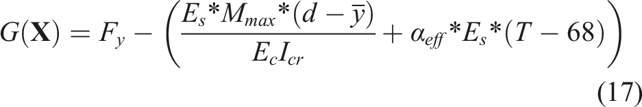$\bar{y} (x)$ , and the moment of inertia of the cracked section, I_cr, before being used to extract q and h_sat from the tilt measurements. Using the estimated loads, the beam model is used to estimate the flexural moment at the base of the wall denoted as M_max. The limit state function is rewritten as:

G (X) = F_{y} - (\frac{E_{s} * M_{\max} * (d - \bar{y})}{E_{c} I_{c r}} + α_{e f f} * E_{s} * (T - 68))

(17)

The first term within the parentheses corresponds to the flexural strain in the lower tensile steel reinforcement bars. The second term estimates the flexural strain based on the effective coefficient of thermal expansion, $α_{e f f},$ estimated from Figure 14. The thermal strain is assumed relative to a temperature of 68°F (20°C). For each day, the Monte Carlo analysis is run 10 million times before convergence is achieved in the estimation of the probability of failure, P_f. The reliability index, $β_{\bar{M}}$ , is plotted for each day in Figure 15 for the case of 0, 10 and 20% section loss in the tensile reinforcement bars at the base of the wall. If no samples of the random variables result in a failed case, the reliability index is not calculated as the probability of failure is effectively zero. The calculated reliability indices for all three assumed steel reinforcement states are above 3.0 which is where load resistance and factor design (LRFD) codes today would aim to achieve. For the 10 and 20 % rebar section loss cases, the reliability index is still above 3, but varies between 3 and 9.

Figure 15.

Daily variation of the reliability index (β) values of the I-696 retaining wall system for 0%, 10% and 20% corrosion states of the steel rebar on the wall tension side.

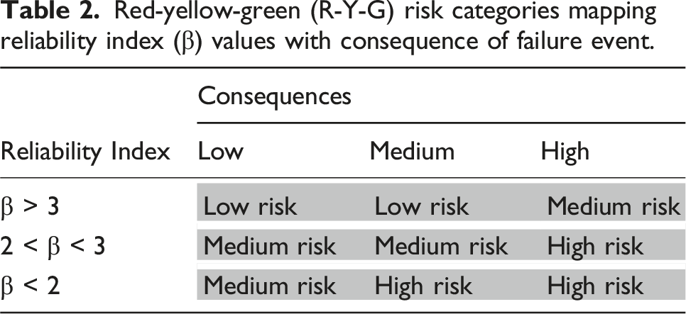
Risk assessment considers the reliability index (providing the probability of exceeding a defined limit state) and the consequences associated with exceeding the limit state with risk is simply the probability times the consequence of exceeding the limit state. Clearly, the probability of failure estimated for each day of monitoring can be used to assess the wall risk. However, the estimation of the consequences of failure remains difficult for the wall owner to do. More practical is for the owner to define if the consequences are low, medium, or high as opposed to defining precisely in the form of failure cost. Similarly, the likelihood of failure can be binned into three categories based on two levels of the reliability index: β_low and β_high. In this study, the upper threshold, β_high, is set to 3 which corresponds to the level of safety sought in retaining wall designs by LRFD. In consultation with the retaining wall owner (i.e., MDOT), the lower threshold, β_low, is set to 2. This established three categories of failure likelihood: low ( $β_{\bar{M}}$ >3), medium (3> $β_{\bar{M}}$ >2), high (2> $β_{\bar{M}}$ ).

Based on the low-medium-high bins for both failure likelihood and consequence of failure, a table defining the perceived risk of the asset is formulated as shown in Table 2. The colors green, yellow, and red correspond to low, medium, and high levels of risk. In the case of the I-696 wall monitored in this paper, its structural function is to support a two-lane service road (Eleven Mile) above an eight-lane freeway (I-696) in a high-volume traffic region (i.e., metropolitan Detroit). This means the wall failure would have a level of high consequence if it failed because of the need to close both the heavily used Eleven Mile Road and I-696 ramp, and potential partial or full closure of eastbound I-696. Given the high reliability, but high consequences, Table 2 would classify this asset as “yellow” indicating more vigilant observation by visual inspection.

Table 2.

Red-yellow-green (R-Y-G) risk categories mapping reliability index (β) values with consequence of failure event.

Reliability Index	Consequences
Reliability Index	Low	Medium	High
β > 3	Low risk	Low risk	Medium risk
2 < β < 3	Medium risk	Medium risk	High risk
β < 2	Medium risk	High risk	High risk

Conclusions

In this paper, a quantitative approach that informs risk-based asset management decision making for retaining wall systems is presented. The approach uses long-term structural monitoring data for the reliability analysis and risk assessment of retaining wall assets. It was motivated by MAP-21 that requires transportation officials to adopt risk management strategies for all highway structures including retaining walls. As a result, an illustrative example of analysis was conducted using monitoring data of a more than 30-year-old classical reinforced concrete (RC) retaining wall system along the I-696 freeway corridor in Southfield, Michigan. The monitoring system installation adopted tiltmeters to measure wall tilt, long-gage strain gages to measure thermal and flexural strains, and thermistors to measure wall temperatures. Specifically, should tilt or strain be measured on irregular basis (for example, manually) or on a short-term basis (say a few weeks or months), the maximum wall response may not be observed. This work shows that short-term variations of the wall tilt and strain can be significant; a more accurate view of wall behavior requires at least 1 year of monitoring to see the full range of seasonal variations. The proposed method does not aim to propose long-term monitoring of all retaining walls; rather, it relies on visual inspections to identify retaining wall systems with levels of distress that warrant structural monitoring to be undertaken. The work develops an analytical framework to process measurement data to identify the reliability of the wall for user-defined limit states. The analytical framework first employs tilt measurements to estimate the lateral pressures on the far-side of the retaining wall using a discretized Euler-Bernoulli beam model of the wall. Estimated lateral pressures are then used to estimate flexural strain using tilt measurements. This allows measured strains associated with thermal loading to be separated from the total strain response. The thermal and flexural response of the wall is then used within a Monte Carlo simulation where wall material and soil properties are randomly sampled from assumed distributions to estimate the probability of exceeding the defined limit state (i.e., probability of failure). This allows the reliability index of the monitored wall to be assessed for each measurement. The work defines an approach to using the reliability index with a qualitative assignment (i.e., low, medium, high) of the consequence of failure to qualitatively assign the retaining wall risk for the asset manager’s decision-making.

Based on the collected wall response data, the I-696 retaining wall system exhibited strong dependence on environmental parameters, most notably temperature. The wall showed higher drifts on its top section as compared to the mid-height. The top section drifts were seasonal with maximum drift in the summer and lower levels of drift experienced in the winter. However, long periods (i.e., multi-day) of rain in the spring season introduced substantial daily and weekly variations in the tilt of the top wall section. Tilt at mid-height of the wall were insensitive to rain and linearly correlated to the wall temperature. To analyze the reliability of the monitored wall, a limit state based on the stress level in the steel reinforcement at the wall base and on the wall tensile (i.e., far-side) side was compared to the yield stress during the Monte Carlo analysis to estimate the probability of failure. While the level of corrosion of the base tensile steel reinforcement is unknown, the work explored the assumption of 0, 10 and 20% section loss with 20% section loss likely a highly conservative assumption of corrosion for a wall of this age. The reliability index ranged from 4.8 to 9.0, 3.8 to 8.1 and 3.2 to 7.7 for the 0, 10 and 20% section loss assumptions. A reliability index above 3.0 is desired based on current practice associated with LRFD-based design codes. Given the high consequences associated with this retaining wall supporting a service road, the risk level is defined as moderate based on the risk assessment framework proposed.

In the future, the general reliability-based asset management framework presented herein can be refined and extended. First, the methodology can be refined by revisiting the assumptions made in the paper. For example, the assumption of a uniform temperature distribution through the thickness of the wall should be revisited with modeling used to assess how a temperature gradient could be considered. Other assumptions about the properties of the soil on the wall backfill can be reviewed to enhance the accuracy of the lateral earth pressure models. The methodology can be extended to other wall types (e.g., tie-back (caisson) supported retaining walls, mechanically stabilized earth (MSE) walls, gravity walls) while protocols that identify which walls in an inventory warrant instrumentation could simultaneously be considered. Finally, additional sensors could be explored to reduce uncertainties inherent to the reliability assessment of the monitored wall while nondestructive evaluation technologies could be used to assess the state of corrosion in the reinforcement to ensure a more accurate reliability analysis is completed.

Footnotes

Acknowledgments

This research project was sponsored by Michigan Department of Transportation (MDOT), Structure Management Section (SMS) under MDOT Project Number 131529-OR15-114. In addition to funding, the authors are grateful to the MDOT team that helped to install the sensors on the retaining wall. The methods, procedures, results, and conclusions of this paper are solely those of the authors and do not represent MDOT.

Declaration of conflicting Interests

The author(s) declared no potential conflicts of interest with respect to the research, authorship, and/or publication of this article.

Funding

The author(s) disclosed receipt of the following financial support for the research, authorship, and/or publication of this article: This work was supported by the Michigan Department of Transportation; 131529-OR15-114.

ORCID iD

Jerome Lynch

References

Admassu

Lynch

Athanasopoulos-Zekkos

, et al. (2019) Long-term wireless monitoring solution for the risk management of highway retaining walls. Proc. SPIE 10971, Nondestructive Characterization and Monitoring of Advanced Materials, Aerospace, Civil Infrastructure, and Transportation XIII. Denver, CO, USA: SPIE, 1097103.

Admassu

Flanigan

Wang

, et al. (2022) Rapid-to-deploy wireless water pressure sensors for the assessment of water distribution systems. In: Accepted for IEEE ISC2 conference, Paphos, Cyprus, 26-29 September 2022.

Aït-Mokhtar

Belarbi

Benboudjema

, et al. (2013) Experimental investigation of the variability of concrete durability properties. Cement and Concrete Research 45: 21–36, Elsevier Science Ltd, U.K.

American Concrete Institute (ACI) (1997) Prediction of Creep, Shrinkage, and Temperature Effects in Concrete Structures. Farmington Hills, MI, USA: ACI Committee, Vol. 209.

Andrade

Alonso

(1996) Corrosion rate monitoring in the laboratory and on-site. Construction and Building Materials 10(5): 315–328, Elsevier Science Ltd, U.K.

Arrayago

Rasmussen

KJR

Real

(2020) Statistical analysis of the material, geometrical and imperfection characteristics of structural stainless steels and members. Journal of Constructional Steel Research 175: 106378, Elsevier Science Ltd, U.K.

Athanasopoulos-Zekkos

Lynch

Zekkos

, et al. (2020) Asset Management for Retaining Walls. Ann Arbor, MI, USA: Final Report Submitted to the Michigan Department of Transportation (MDOT) – ORBP. Number OR15-114.

Basheer

Najjar

(1996) Reliability-based design of reinforced earth retaining walls. Transportation Research Record 1526: 64, Washington, DC, USA.

Berwanger

Sarkar

(1976) Thermal expansion of concrete and reinforced concrete. ACI Journal 73(11): 618–621.

10.

Bosch

. BNO055: Intelligent 9-axis Absolute Orientation Sensor. Sensor Datasheet - BST-Bno055- DS000-14. Reutlingen, Germany: Bosch Sensortec GmbH, 2016.

11.

Bournonville

Dahnke

Darwin

(2004) Statistical analysis of the mechanical properties and weight of reinforcing bars. In: Structural Engineering and Materials Laboratory. Lawrence, KS, USA: University of Kansas. Report 04-1.

12.

Bridge Diagnostics Inc (BDI) (2006) 5.2 BDI Strain Transducer – ST350. Boulder, CO, USA: STS - WiFi Operations Manual.

13.

Chu

(1991) Rankine’s analysis of active and passive pressures in dry sands. Soils and Foundations 31(4): 115–120.

14.

Coduto

(2001) Foundation Design: Principles and Practices. 2nd edition. London, UK: Pearson.

15.

DeMarco

Keough

Lewis

(2010) Retaining Wall Inventory and Assessment Program (WIP) National Park Service Procedures Manual. Washington, DC, USA: Federal Highway Administration (FHWA), U.S. Department of Transportation, 188. Publication No. FHWA-CFL/TD-10-003.

16.

Elsener

Andrade

Gulikers

, et al. (2003) Half-cell potential measurements – potential mapping on reinforced concrete structures. Materials and Structures 36(4): 461–471.

17.

Federal Highway Administration (FHWA) (2008) Earth Retaining Structures and Asset Management. Washington, DC, USA: Department of Transportation. Publication No. FHWA-IF-08-014, U.S.

18.

Federal Highway Administration (FHWA) (2009) Design and Construction of Mechanically Stabilized Earth Walls and Reinforced Soil Slopes: Volume II. Washington, DC, USA: Federal Highway Administration. Publication No. FHWA NHI-10-025.

19.

Federal Highway Administration (FHWA) (2014) 2014 Transportation Asset Management Peer Exchange – Preparing for MAP-21 Implementation. Washington, DC, USA: U.S. Department of Transportation. Publication No. FHWA–HIF–14–013.

20.

Federal Highway Administration (FHWA) (2017) Incorporating risk management into transportation asset management plans. In: Office of Asset Management. Washington, DC, USA: U.S. Department of Transportation.

21.

Flanigan

Lynch

(2018) Community engagement using urban sensing: technology development and deployment studies. In: 25th international workshop on intelligent computing in engineering. Lausanne, Switzerland, June 10-13, 2018.

22.

Flanigan

Lynch

Ettouney

(2020) Quantitatively linking long-term monitoring data to condition ratings through a reliability-based framework. In: Structural Health Monitoring. Thousand Oaks, CA, USA: Sage Publishing.

23.

Frangopol

Strauss

Kim

(2008) Bridge reliability assessment based on monitoring. Journal of Bridge Engineering 13(3): 258–270, ASCE.

24.

Fujino

Siringoringo

(2011) Bridge monitoring in Japan: the needs and strategies. In: Structure and Infrastructure Engineering. Oxfordshire, UK: Taylor & Francis, 597–611.

25.

Goh

ATC

Kulhawy

(2005) Reliability assessment of serviceability performance of braced retaining walls using a neural network approach. International Journal for Numerical and Analytical Methods in Geomechanics 29: 627–642, John Wiley & Sons, Hoboken, NJ, USA, 2005.

26.

Hou

Lynch

Ettouney

, et al. (2020) Partial composite action and durability assessment of slab-on-girder highway bridge decks in negative bending using long-term structural monitoring data. Journal of Engineering Mechanics 146(4): 04020010, ASCE.

27.

Jansson

(2007) Rotation/movement of Retaining Wall, I-696 at Evergreen Road. Lansing, MI: Office Memorandum, Michigan Department of Transportation. Technical Investigation TI-2103.

28.

Jensen

(2009) Inspector’s Manual for Mechanically Stabilized Earth Walls. Ord, NE, USA, Nebraska Department of Roads (NDOR), 36. Publication No. SPR- P1(09) P320.

29.

Kalenjuk

Lienhart

Rebhan

, et al. (2019) Largescale monitoring of retaining structures: new approaches on the safety assessment of retaining structures using mobile mapping. Proc. SPIE 10970, Srensos and Smart Structures Technologies for Civil, Mechanical, and Aerospace Systems. Denver, CO, USA: SPIE, 109700T.

30.

Kim

Hummer

Gabr

, et al. (2009) Asset Management Inventory and Data Collection. Raleigh, NC, USA: North Carolina Department of Transportation (NCDOT), 286. Publication No. FHWA/NC/2008-15.

31.

Koerner

(2011) Recommended Layout of Instrumentation to Monitor Potential Movement of MSE Walls, Berms, and Slopes. Folsom, PA, USA: Geosynthetic Institute.

32.

Koloski

Schwarz

Tubbs

(1989) “Geotechnical properties of geologic materials,” Engineering geology in Washington – Volume I. Publisher: Washington Olympia, WA, USA division of geology and earth resources .

33.

Kurata

Spencer

Ruiz-Sandoval

(2005) Risk monitoring of buildings with wireless sensor networks. Structural Control and Health Monitoring 12(3): 315–327.

34.

Kurata

Kim

Lynch

, et al. (2013) Internet-enabled wireless structural monitoring systems: development and permanent deployment at the new carquinez suspension bridge. Journal of Structural Engineering 139(10): 1688–1702, ASCE.

35.

Low

(2005) Reliability-based design applied to retaining walls. Géotechnique 55(1): 63–75, Institution of Civil Engineers, London, U.K.

36.

Michigan Department of Transportation (MDOT) (1986) 63102 – I-696 Retaining Wall Details (Plan and Profile). Lansing, MI, USA: Working Drawings.

37.

Michigan Department of Transportation (MDOT) (2013) Preliminary Findings of Retaining Wall Investigations. Lansing, MI, USA: Office Memorandum.

38.

Mirza

MacGregor

(1979) Variability of mechanical properties of reinforcing bars. Journal of the Structural Division 105(5): 921–937.

39.

Naval Facilities Engineering Command (NAVFAC) (1986) Soil Mechanics – Design Manual 7.01. Alexandria, VA, USA: United States Navy.

40.

Oregon Department of Transportation (ODOT) (2007) ODOT Specifications – 2007. Specifications, Section 00596. Salem, OR, USA: ODOT, 11.

41.

Oskouie

Becerik-Gerber

Soibelman

(2016) Automated measurement of highway retaining wall displacements using terrestrial laser scanners. Automation in Construction 65: 86-101, Elsevier Science Ltd.

42.

Pakzad

Fenves

Kim

, et al. (2008) Design and implementation of scalable wireless sensor network for structural monitoring. Journal of Infrastructure Systems 14(1): 89–101.

43.

Straser

Kiremidjian

Meng

, et al. (1998) Modular, wireless network platform for monitoring structures. Proceedings of the 16th international modal analysis conference (IMAC), Santa Barabara, CA, 2 - 5 February 1998 1: 450–456.

44.

Swartz

Jung

Lynch

, et al. (2005) Design of a wireless sensor for scalable distributed in-network computation in a structural health monitoring system. In: Proceedings of the 5th international workshop on structural health monitoring, Stanford, CA, 12 – 14 September 2005, 1570–1577.

45.

Swartz

Lynch

Zerbst

, et al. (2010) Structural monitoring of wind turbines using wireless sensor networks. Smart Structures and Systems 6(3): 183–196.

46.

Uddin

Hudson

Haas

(2013) Public Infrastructure Asset Management. 2nd edition. New York, NY, USA: McGraw Hill.

47.

Vessely

Robert

Richrath

, et al. Geotechnical Asset Management for Transportation Agencies. Volume 2: Implementation Manual, NCHRP Research Report 903, National Academies, Washington, DC, USA, 2019.

48.

VicRoads Technical Services (2014) Road Structures Inspection Manual. Victoria, Australia: State Government of Victoria.

49.

Walters

Collins

Funk

, et al. (2016) Colorado Retaining and Noise Walls Inspection and Asset Management Manual. Denver, CO, USA: Colorado Department of Transportation (CDOT), 300.

50.

Washington State Department of Transportation (WSDOT) (2011) Geotechnical Design Manual. Olympia, WA, USA: WSDOT. Publication No. M 46-03.04, Environmental and Engineering Programs.

51.

Weather Underground (2022) Detroit, Michigan. The Weather Company (TWC). San Francisco, CA: Weather Underground. https://www.wunderground.com/weather/us/mi/detroit (accessed 20 August 2022).

52.

Tan

Lin

, et al. (2022) Development of a monitoring and warning system based on optical fiber sensing technology for masonry retaining walls and trees. Journal of Rock Mechanics and Geotechnical Engineering. Amsterdam, Netherlands: Elsevier, 14, 1064–1076.

53.

Yanev

(2007) Bridge Management. Hoboken, NJ, USA: John Wiley and Sons.

54.

Yen

Ravani

Lasky

(2011) LiDAR for data efficiency. Olympia, WA, USA: Washington State Department of Transportation (WSDOT), 101. Office of Research and Library Services, Report No. WA-RD 778.1.

55.

Zhang

Kurata

Lynch

(2017) Long-term modal analysis of wireless structural monitoring data from a suspension bridge under varying environmental and operational conditions: system design and automated modal analysis. Journal of Engineering Mechanics 143(4): 04016124, ASCE.

56.

Zonta

Zandonini

Bortot

(2007) A reliability-based bridge management concept. Structure and Infrastructure Engineering 3(3): 215–235, Taylor & Francis.

57.

Zonta

Glisic

Adriaenssens

(2014) Value of information: impact of monitoring on decision-making. Structural Control and Health Monitoring 21: 1043–1056.