




Abstract
Due to variations in wind speed profiles along the length of bridge stay cables, vortex-induced vibrations (VIV) exhibit multimodal characteristics, presenting challenges for VIV identification. Currently, the VIV identification is concentrated on the stable stage of VIV, lacking an available early warning system for detecting the initial developing stage of VIV. In this study, a deep learning-based approach that integrates energy distribution ratio features derived from frequency band wavelet packet decomposition to recognize VIV of stay cable was proposed. Firstly, vibration characteristics induced by vortices in cable-stayed bridges were analyzed based on field monitoring data from the bridge health monitoring system, aiming to propose suitable feature indicators for VIV identification. Secondly, using root mean square as label classification, a deep learning model was constructed, incorporating convolutional neural networks, long short-term memory networks, and attention mechanisms. Finally, four different stages in the evolution of stay cables VIV were identified utilizing field monitoring datasets to analyze the optimal parameter. Meanwhile, effective early warning recognition was achieved through the classification and recognition of confusion matrix. This study provides technical support for early warning systems and structural condition assessment concerning bridge stay cable VIV.
Keywords
Introduction
Cable-stayed bridges are highly favored by bridge constructors due to the superior attributes such as long spanning capacity, elegant design and well-established construction methods. Stay cables constitute a critical component of cable-stayed bridges and are particularly sensitive to wind-induced excitations, with a pronounced susceptibility to vortex-induced vibrations (VIVs). Numerous scholars have conducted research on stay cables VIVs based on observations of prototype bridge cables. Ge and Chen (2019) analyzed the acceleration data of the stay cables of the Sutong Bridge based on monitoring data for 6 months, revealing that stay cables VIVs occur only at wind speeds ranging from 4 m/s to 8 m/s. Matsumoto et al. (2003) established a large-scale stay cable model for observations and discovered cable flutter and multimodal VIV phenomena. Zuo et al. (2010) conducted on-site monitoring of the stay cables of the Fred Hartman Bridge in the United States and observed multimodal VIVs in the cables. It indicates that the occurrence probability of VIVs in stay cables is notably high and is closely associated with the wind environment and structural properties of cables through above analysis. Frequent and continuous VIV will cause structural fatigue damage and shorten the service life of the stay cable (Argentini et al., 2016), significantly affecting the operational safety of the cable-stayed bridge.
Stay cables VIVs result from the periodic shedding of vortices generated as wind flows over the surface of cables, which create pressure variations. When the shedding frequency approaches or matches the natural frequency of cables, resonance will occur, typically manifested as amplitude-limited vibrations. To elucidate the principles of VIVs in stay cables by investigating the mechanisms of flow interaction with cylindrical bluff bodies, methods such as flow field analysis, wind tunnel experiments and computational fluid dynamics simulations (CFD) have employed by scholars. Williamson (1996) and Wu et al. (2006) conducted flow field visualization experiments and further Particle Image Velocimetry tests, revealing a correlation between the occurrence of wake flow instability behind a cylinder and the incoming Reynolds number (Re). Jing et al. (2023) used CFD method to install C-rings on slender cylindrical structures to reduce the effect of vortex-induced vibration. Xu et al. (2024) used the CFD method to suppress VIV of a cylinder by using a traveling wave wall flow control method. Chen et al. (2015) investigated the VIVs response of cables under different wind speed profiles through wind tunnel experiments, founding that the occurrence of multi-modal VIVs in the cables is related to the distribution of oncoming flow velocities. Liu et al. (2022) investigated the suppressive effects of different helical devices on high-mode VIVs in stay cables through wind tunnel experiments, ultimately obtaining effective parameters for the suppression of VIVs by the helical devices. However, reduced-scale experiments fail to comprehensively and effectively replicate the operational conditions of real bridge stay cables, thereby the experimental exploration of VIVs in stay cables has been somewhat constrained. Consequently, field studies on prototype bridge stay cables are of great necessity.
Field studies of stay cables in prototype bridges have revealed that the field wind conditions for cables are considerably more complex compared to wind tunnel experiments. Furthermore, there are significant differences in the dynamic characteristics of stay cables in the actual cable models compared to experimental cables. He et al. (2022) conducted research on the identification of single-mode VIVs in stay cables using acceleration data, in conjunction with features from both the frequency domain and the complex domain. Kim et al. (2022) proposed a modal decomposition method that includes automatic peak picking and continuous band-pass filtering to reveal the relationship between the shedding frequency of stay cables and the corresponding critical wind speeds. Moreover, through damping identification, it was discovered that there is a strong correlation between the amplitude of vibrations during VIVs in stay cables and the damping. Denoël et al. (2017) recorded and analyzed multi-modal VIVs in 20 pairs of extra-long stay cables, a model proposed by Vickery et al. (1983a, 1983b) was referenced, which indicated vortex shedding occurs within a certain bandwidth. Besides, they made a pioneering attempt to determine the model parameters from full-scale measurements. However, the aforementioned studies only explored the correlation between wind parameters and vibration parameters during VIVs in stay cables while specific comprehensive and effective identification methods and strategies were not proposed. Therefore, it is necessary to organize and analyze a significant amount of monitoring data for stay cables, aiming to derive an effective identification method for VIVs in stay cables.
Dealing with the large volume of monitoring data from actual bridge stay cables and accurately extracting, categorizing, and identifying VIVs in cables has emerged as a significant challenge. Machine learning (ML) methods have proven effective in addressing this issue. ML has found widespread applications across various fields, with scholars utilizing it for complex feature extraction and classification tasks. In the field of aeroelastic vibrations induced, researchers have applied ML for modeling and analysis of main span VIVs. Yan et al. (2022) utilized computer vision combined with a new Bayesian inference method to predict and analyze the vorticity vibration of long-span bridges. Li et al. (2018) employed the decision tree in combination with a support vector machine to separately identify main span VIVs based on wind characteristics and predict the root mean square of acceleration during VIVs. Kim (2022) and Lim (2022) proposed a generic framework that employs various ML methods to predict main span VIVs in cases with limited VIVs data. Then, the proposed framework was validated, which yielded effective predictions of VIVs. Additionally, an automatic classification method for VIVs using supervised self-labeling techniques was developed. The Deep Neural Network (DNN) model was trained with labeled data, and the results were validated, yielding accurate identification. Based on the aforementioned analysis, ML has found substantial applications in the identification of girder VIVs. Although ML has demonstrated effectiveness in identifying of VIVs in girder, there remains a need for research on the identification of VIVs in stay cables. The primary challenge arises from the fact that VIVs in stay cables are often multi-modal, presenting difficulties in conducting feature analysis within the frequency domain. Consequently, there are fewer characteristic parameters compared to VIVs in girder. Based on energy decomposition using wavelet packet analysis, this paper effectively integrated the energy distribution ratio as a feature indicator for deep learning (DL) with multi-modal characteristics. By introducing additional feature indicators, it surpasses the use of the root mean square of acceleration as the sole criterion for determining the occurrence of VIVs, which facilitates the analysis of the developing stages of VIV, providing a predictive function. Furthermore, in contrast to conventional supervised classification methods in ML, the challenge about frequently encounter limitations in the input dimensions of feature parameters can be overcome by DL. Meanwhile, DL exhibits superior recognition accuracy compared to traditional ML methods.
The rest of the paper is organized as follows. The characteristics of VIVs in stay cables were analyzed based on the wind field and vibration data from 2010 to 2011. Then, DL methods were applied to construct a model for the identification of VIVs in stay cables. The characteristics of VIVs in stay cables, including wind speed, wind direction, vibration acceleration, and power spectral features, were analyzed. Subsequently, energy distribution through wavelet packet decomposition was used to differentiate between VIVs and non-VIVs, and feature indicators were introduced. The index of root mean square (RMS) of acceleration was introduced as the basis for label classification. Meanwhile, convolutional neural networks (CNN)-long short-term memory networks (LSTM)-Attention mechanism was employed to model the identification of VIVs in stay cables, aiming to obtain the identification parameter. Finally, the identification results demonstrated the feasibility and effectiveness of the proposed approach.
Characteristics analysis of VIVs in stay cables
Source of field monitoring data
This study was based on the monitoring data of the cables of a cable-stayed bridge in Zhejiang Province, as shown in Figure 1(a). The cable-stayed bridge boasts a main span of 602 m, a bridge deck width of 30.1 m, and a height of 3 m, supported by 168 stay cables distributed on both sides. The VIVs of the cable CAC20 of the bridge occurred several times, so field monitoring data of the CAC20 was collected to analyze. Table 1 lists the parameters of the stay cable (CAC20). Figure 1(b) illustrates the location of the monitoring points. Wind speed measurements were conducted using three-dimensional ultrasonic anemometers (UA1 and UA2) deployed on the bridge deck and propeller-vane anemometers (AN1 and AN2) deployed on the bridge tower top. The single axial accelerometer installed on the stay cable CAC20 measured vibrations of the cable plane and was positioned 6 m above the bridge deck. The accelerometer has a sensitivity of 1000 mV/g, a frequency range of 0-400 Hz, and a sampling frequency of 100 Hz. The bridge deck anemometers were installed at a height of 6 m above the bridge deck, and has a wind speed recording range of (0.1-60) m/s, with a sampling frequency of 32 Hz. The tower-top anemometers were located 2.1 m above the tower top, measuring wind speeds in the range of (0-80) m/s and wind directions from (0-360) degrees, with a sampling frequency of 1 Hz. The anemometer at the bridge deck was installed at a height of 65 m above the ground, the anemometer at the top of the tower was installed at a height of 212.1 m above the ground, and the bridge deck is at a height of 59 m. Bridge location and sensor distribution. CAC20 Stay Cable Parameters.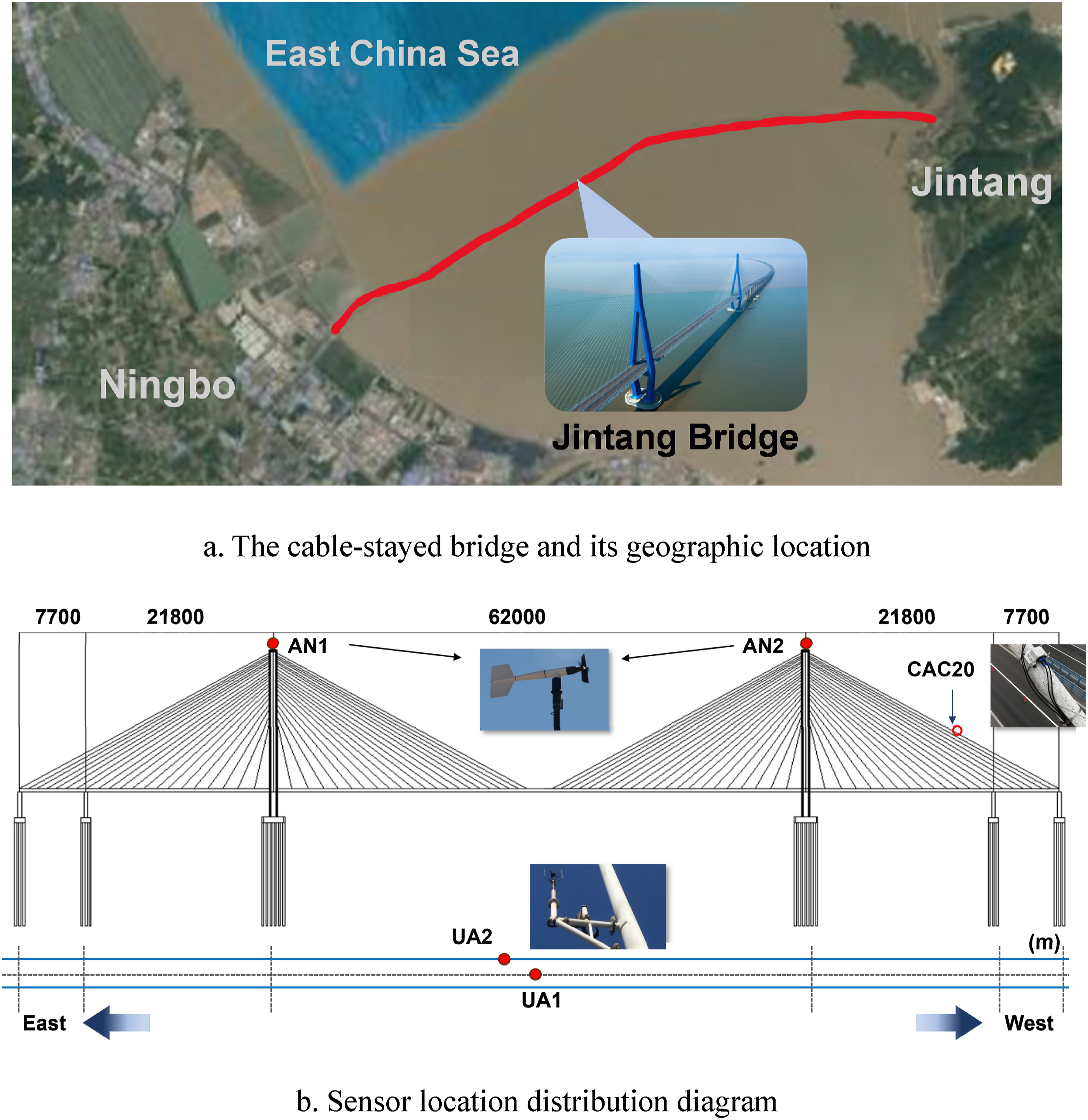

Mechanism of VIVs in stay cables
To validate that the data acquired from the structural health monitoring system pertains to VIV of the stay cable, a model for the stay cable under the influence of incoming wind flow was established. Given the considerable length of the actual stay cable, wind speed undergoes significant variations with changes in height. Therefore, it is crucial to account for the impact of height on wind speed. The relationship between wind speed and height can be expressed as:
Due to the consideration of height effects, the Re also varies with different wind speed profiles. Therefore, the Strouhal number at different heights can be calculated using the following equation (W. L. Chen et al., 2019; Norberg, 2003):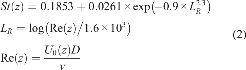
Therefore, the shedding frequency 
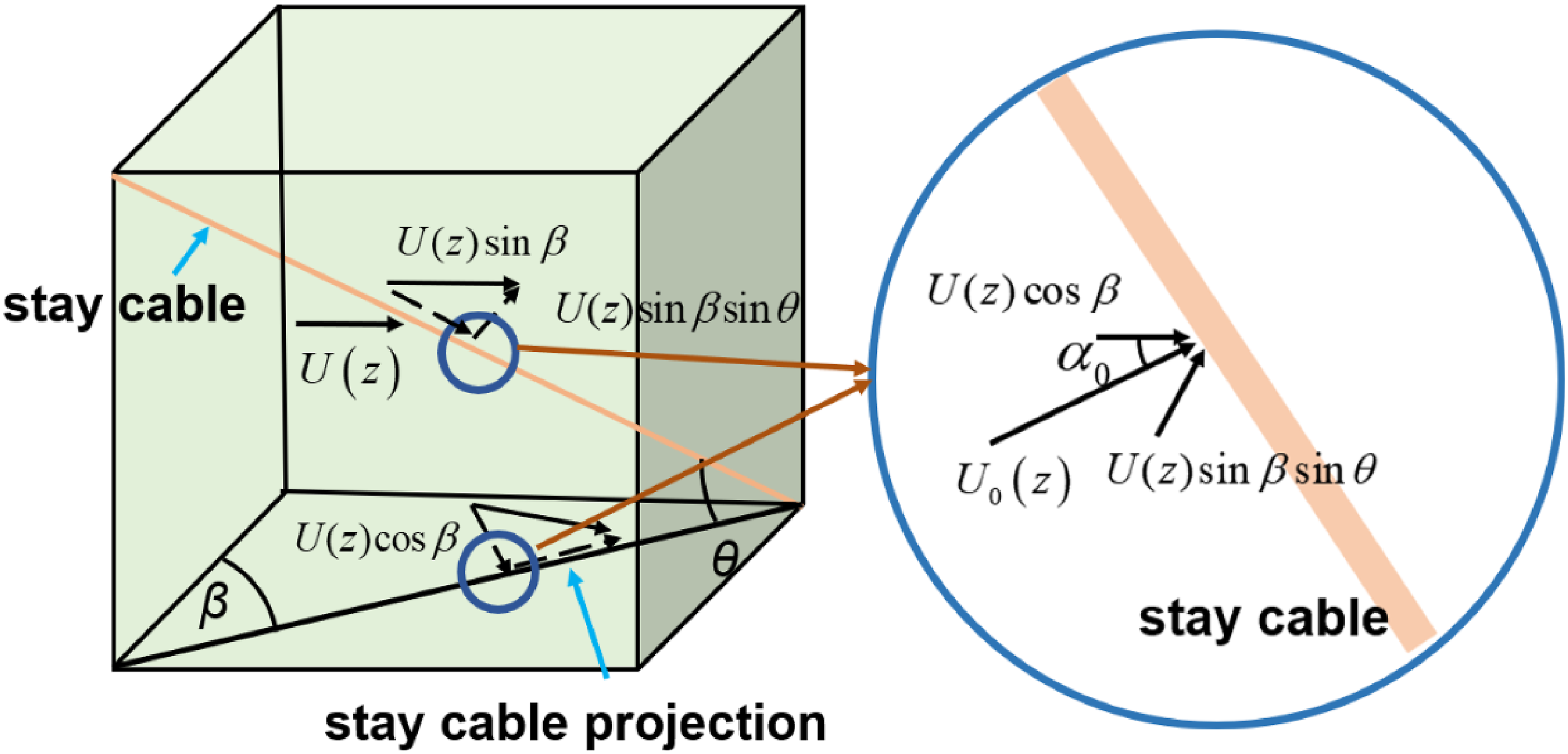
By selecting a terrain roughness value of 0.125, typical for coastal bridges, the mean wind speeds at different heights for the stay cables can be calculated. However, in practice, the wind does not usually act directly vertically on the plane of the stay cables. As shown in Figure 2, the incident wind speed is decomposed into two components perpendicular to the span of cable, represented as U(z)cos(β) and U(z)sin(β)sin(θ). The wind angle of attack can be obtained as: The incoming wind acts on the stay cable.
In this study, VIVs data from July and August of 2010, as well as March and April of 2011 were proposed to establish the relationship between the shedding frequency of the bridge deck and tower-top wind speeds and the vibration frequency of stay cables under VIV conditions. Based on above analysis, the comparison of the shedding frequency and the main mode frequency under VIVs is presented in Figure 3. It can be observed that the overall shedding frequency trend closely aligns with the trend of the main mode frequency of stay cables. Comparison of frequency change.
Figure 4(a) illustrates the relationship between the dominant frequency and the wind velocity lock-in region during VIVs of stay cables at different wind speeds. Ge et al. (2019)converted the wind speed of the bridge tower and the bridge deck into the wind speed at the midpoint of the cable, which is considered to be more reasonable. Therefore, the field wind speed acting at the midpoint of the stay cables, which took wind direction into account, was calculated based on the inflow wind conditions depicted in Figure 2. The analysis of the field monitoring data indicates a positive correlation between inflow wind speed and changes in the dominant mode of VIVs, with the wind speed lock-in range is observed, as shown in Figure 4(b). The shedding frequency of vortices rises with the increase of wind speed, thereby eliciting higher-order modes. Based on the aforementioned analysis, it is evident that the selected data pertains to the VIVs of stay cables. The correlation between the wind speed and the dominant frequency of stay cables for VIV, (a) Vortex-shedding frequency and wind speed lock-in range, (b) The relationship between wind speed and dominant frequency of monitoring data.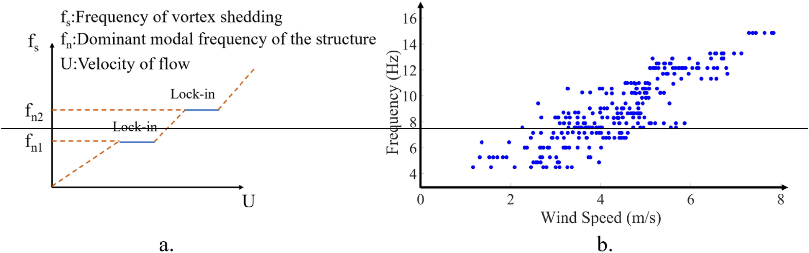
Phenomenon of VIVs in stay cables
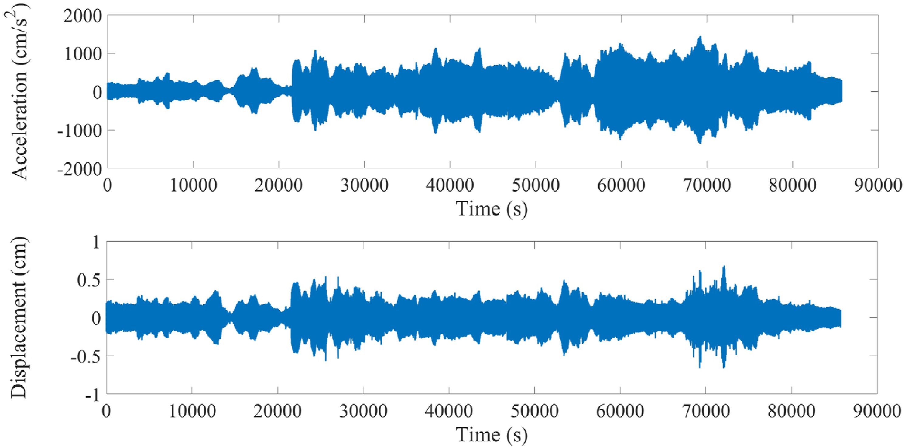
Based on the field monitoring data of cable CAC20, the characteristics of wind speed, wind direction, displacement, and acceleration were analyzed under both VIVs and non-VIVs conditions. The wind data for April 7, 2011, is illustrated in Figure 5. The wind speed at the top of the bridge tower exceeds that on the bridge deck, with the wind direction approximately perpendicular to the bridge axis. Figure 6 presents the acceleration and displacement on April 7, 2011, it can be observed that the vibration amplitude after 20,000s is significantly larger than the normal vibration levels, indicating that the VIV of the cable is most easily induced when the wind direction is perpendicular to the bridge axis. Wind data on April 7, 2011, (a) Wind speed and wind direction at bridge tower-top, (b) Wind speed and wind direction at bridge deck. Acceleration and displacement time history on April 7, 2011.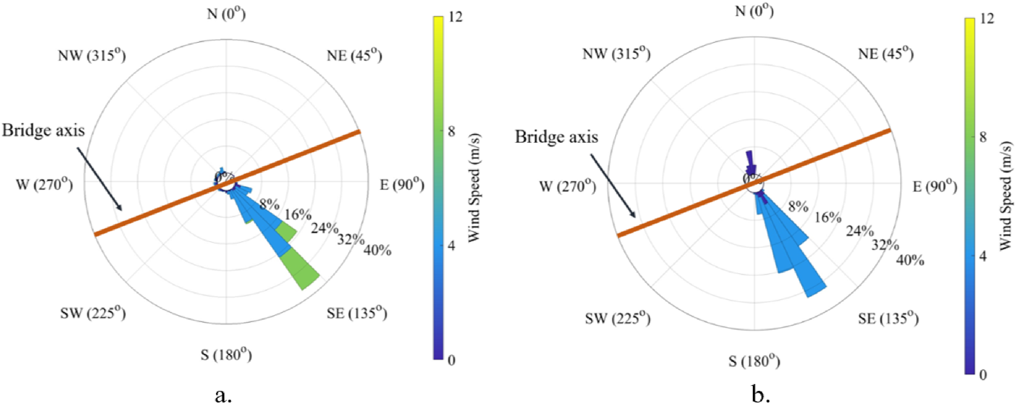
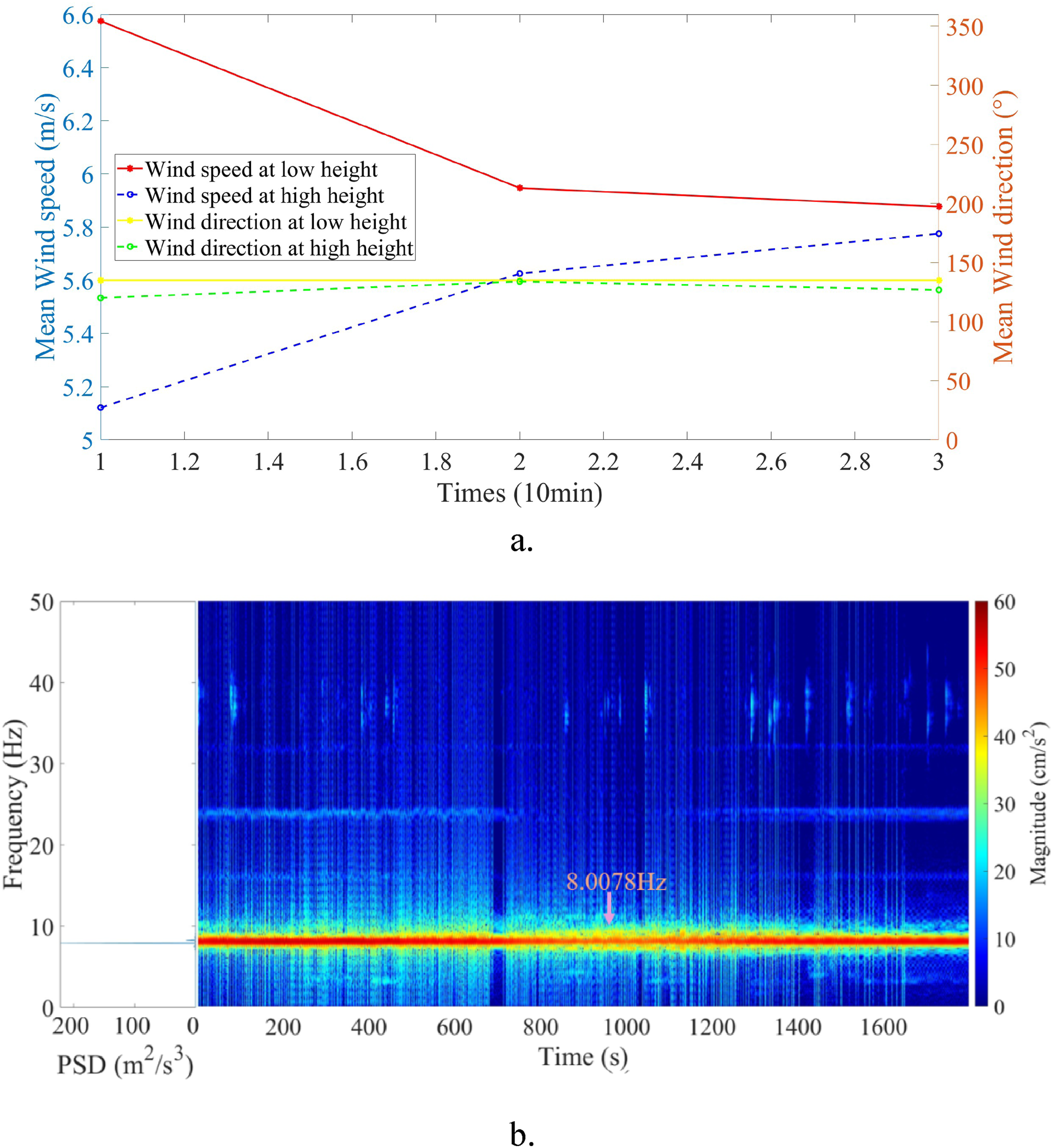
Figures 7 and 8 illustrate the wind field and acceleration characteristics in the multi-mode and single-mode VIV of the cable, respectively. The acceleration is given in the form of power spectral density (PSD) and short-time Fourier transform (STFT). As shown in Figure 7, spectral analysis of the acceleration data reveals the dynamic evolution of the VIV dominant mode in the cable. When VIVs occurs, the wind speed and direction of the bridge deck and the tower top are closely aligned. The frequency of the dominant mode of VIV in the cable rises with the increase of wind speed, gradually evolving from the 15th order to the 19th order. Notably, it is found that the stay cable not only exhibits multi-mode VIV, but also undergoes single-mode VIV. As shown in Figure 8, single-mode VIV of the cable occur when the wind speed of the bridge deck and the tower top are close, and the wind profile demonstrates minimal variation, approximating a uniform flow condition. Multi-mode VIV: (a) Mean wind speed and direction, (b) The PSD and STFT of acceleration. Single-mode VIV: (a) Mean wind speed and direction, (b) The PSD and STFT of acceleration.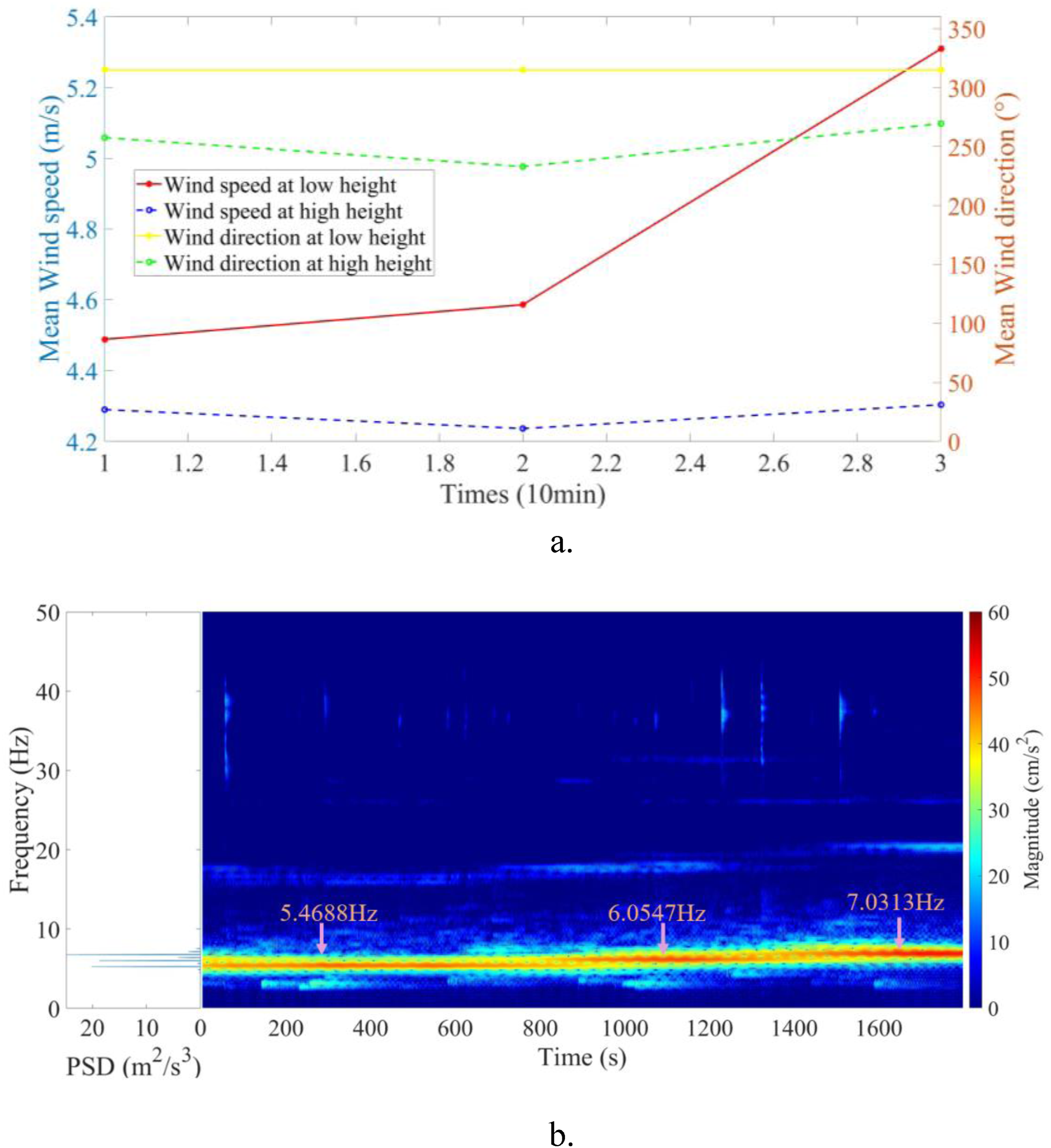
Energy analysis of VIVs based on wavelet packet decomposition
In contrast to the single-mode VIVs characteristics observed in the girder, the frequency domain features of VIVs in stay cables are more closely resemble those observed in non-VIVs, with both exhibiting multimodal characteristics, complicating the quantitative analysis of energy distribution in VIVs in stay cables. The characteristics of frequency domain during VIVs in stay cables primarily manifest as coupling between the main mode and sub modes, typically with adjacent modal orders. Exploiting above feature, wavelet packet decomposition theory was employed to represent the frequency domain within bands. Through the analysis of energy distribution in various frequency bands of stay cables, feature extraction of energy distribution during VIVs process of stay cables was achieved.
Wavelet packet decomposition theory
Wavelet analysis extends Fourier analysis for the frequency domain analysis of signals. Wavelet packet analysis, derived from wavelet analysis, has found widespread application, especially in signal denoising. Compared to wavelet analysis, wavelet packet analysis provides a more precise resolution for high-frequency components in vibration signals and allows for simultaneous decomposition of both high and low-frequency components. Through wavelet packet decomposition, vibration frequency bands will be divided into multiple levels, offering more accurate time-frequency characteristics than wavelet transforms. Guo et al. (2020, 2021)utilized wavelet transformation and wavelet packet energy analysis to characterize the vibration response of sea-crossing bridges. It can be concluded that wavelet packet analysis effectively assesses the structural health of bridge while exhibiting significant advantages in data processing such as stay cable vibration signals.
Wavelet packet analysis is essentially an extension of orthogonal wavelets, characterized by the combination of different wavelet basis functions. It inherits the orthogonality and time-frequency characteristics of wavelet basis functions. Given a signal Y, the sampling frequency is f, and after preprocessing, i-layer wavelet packet decomposition is performed to obtain 2
i
sub-bands. The signal Y can be expressed as:
Figure 9 presents the process of three-level wavelet packet decomposition. The signal S is initially decomposed into an approximation signal P1 and a detail signal Q1 using low-pass and high-pass filters. Subsequently, the decomposition process is iteratively repeated, exemplifying the three-level decomposition, ultimately yielding a total of eight signals. Depending on the signal characteristics and the desired outcome of the signal decomposition, the number of decomposition levels can be adjusted to meet specific requirements. However, determining the appropriate Wavelet generating function and the number of decomposition levels to achieve optimal results are issues for consideration (Sang, 2012). Wavelet packet decomposition of a signal.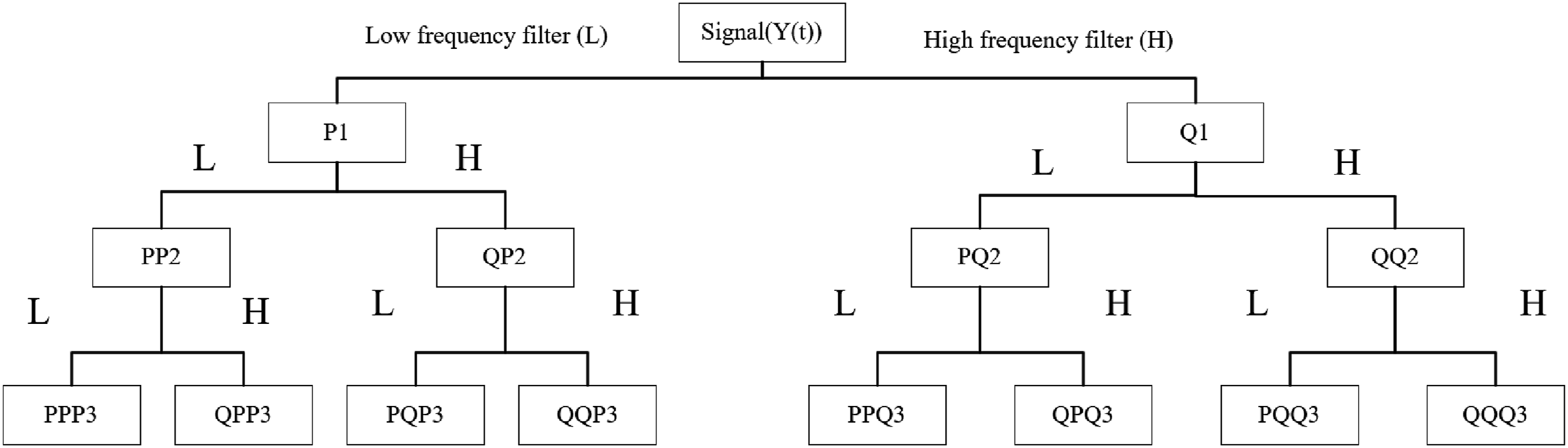
To address above issues, the norm entropy 
The energy of the ith level signal component is typically defined as given by equation (7):
The proportion 
Multiscale acceleration signal decomposition
In the study of the dynamic response of stay cables based on wavelet packet energy, the Daubechies (dbN) family is a crucial wavelet basis function. Xia et al. (Xia et al., 2021) utilized the dbN family functions as wavelet basis functions, using the total energy variation rate of the wavelet packet as a damage indicator, and combined it with a neural network to detect cables with varying degrees of damage. Guo et al. (2021) analyzed the dynamic response characteristics of stay cables measured under typhoon conditions using the dbN family functions as the basis functions for wavelet packet energy. And the frequency band distribution of the wavelet packet energy is an important indicator of the dynamic response of the cables. Considering the advantages of the dbN family, which includes features like asymmetry, orthogonality, and biorthogonality, the dbN family was selected as the wavelet basis functions for the analysis. In the process of discrete wavelet transformation, excessive decomposition levels can result in overly wide frequency bands, leading to the waste of computational resources. In contrast, excessively small frequency bands may overlook higher-frequency components and result in data loss. To determine the most appropriate number of wavelet decomposition levels, various levels of wavelet packet multiscale decomposition were applied to the original signal. Then compared results with the values of the aforementioned norm entropy, enabling the identification of the most suitable multiscale decomposition levels. Through above analysis, a wavelet decomposition level between three and five was considered. Figure 10 depicts the first eight detail signals obtained from the wavelet decomposition of the original acceleration signal after five levels of decomposition. Since stay cables experience VIVs at higher modes, the energy is mainly distributed in the middle to high-frequency bands obtained through wavelet decomposition. The original acceleration signal of the stay cable compared with the multiscale decomposed signals, (a) Acceleration signal, (b) Decomposed acceleration signals.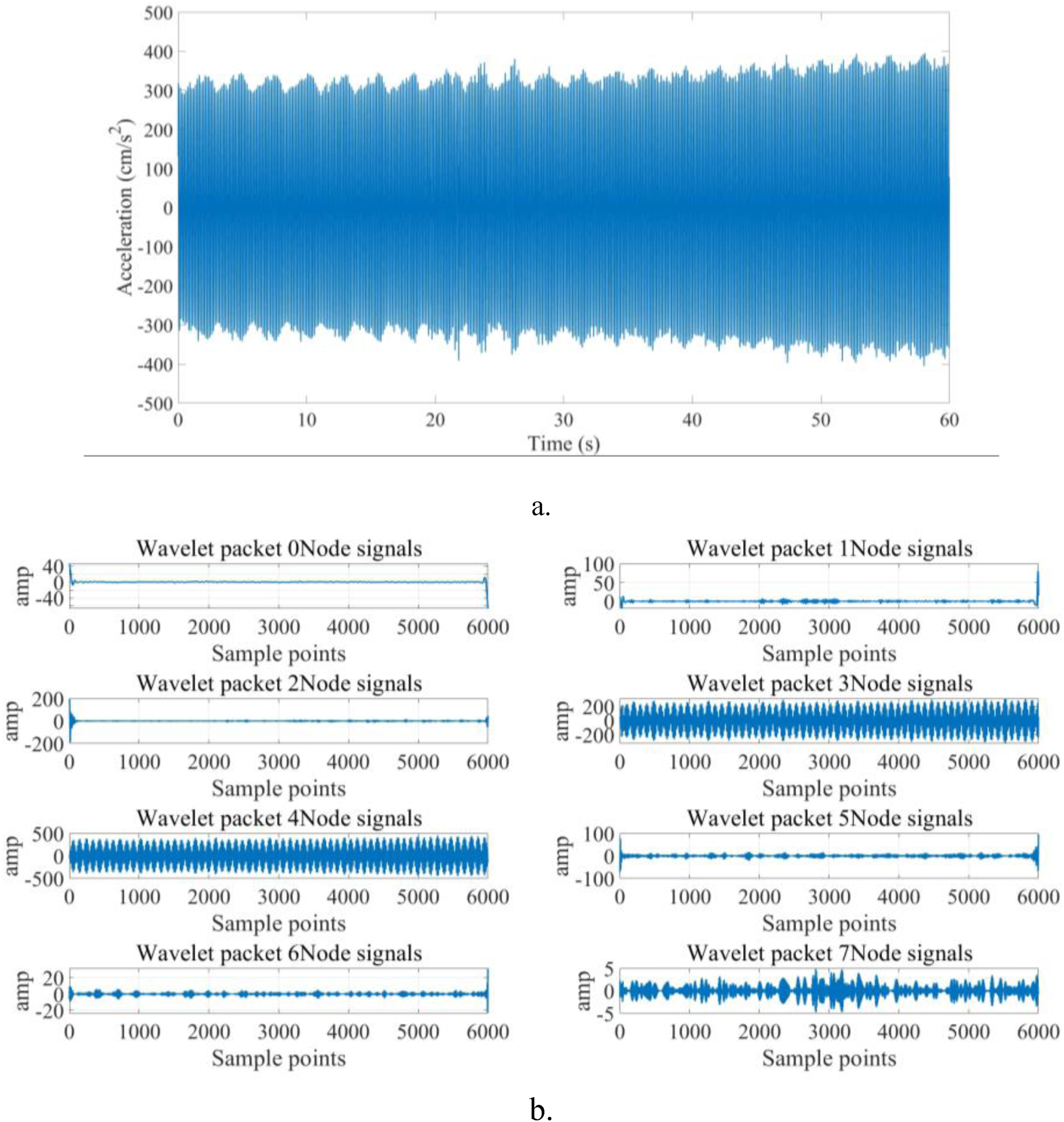
Values of

VIVs energy distribution analysis
The proportion of wavelet packet energy during VIVs of stay cable shows significant differences compared to normal vibrations. As illustrated in Figures 11–13, the power spectral frequency distribution of normal vibrations is more dispersed without prominent peaks, and the amplitude of peak energy is significantly lower than VIVs. Comparing the energy distribution within frequency bands, it reveals that the distribution pattern within the frequency bands has a similar trend to the energy distribution in the power spectrum. The energy distribution within the frequency bands can more intuitively represent the energy distribution within different frequency ranges, facilitating a quantitative analysis of the energy differences between VIVs and normal vibrations. The vibration frequencies of stay cables and their corresponding energy proportions in frequency bands during normal vibrations. The vibration frequencies of stay cables and their corresponding energy proportions in frequency bands during single-mode VIVs. The vibration frequencies of stay cables and their corresponding energy proportions in frequency bands during multi-mode VIVs.


The energy of normal vibrations in stay cables is concentrated in the low-frequency and high-frequency bands, with a relatively lower proportion in the mid-frequency band. The overall energy distribution broad, with each frequency band generally accounting for less than 20% of the total energy. During VIVs, the energy distribution exhibits similar characteristics whether in single-mode or multi-mode vibrations. The energy proportion distribution typically involves pairs of adjacent frequency bands, with two bands accounting for over 85% of the total energy within the bands.
The distribution of energy proportions in single-mode vibrations is not dominated by the single frequency band, which is related to variations in the wind profile. Consequently, when stay cables experience single-mode VIVs, adjacent modes may appear next to the primary mode. Although the primary mode captures most of the energy in the frequency domain, the wavelet packet transform decomposes the signal hierarchically, allowing for independent analysis of energy in different frequency bands. If the original signal contains multiple frequency components, the frequency components can be concentrated in different wavelet packet bands after decomposition. Compared to the traditional fast Fourier transform, the wavelet packet transform can capture more dominant frequency components.
To investigate the disparity in frequency band energy of wavelet packets between VIV and normal vibration, a complete VIV event of a stay cable was utilized for analysis. As illustrated in Figure 14, the entire VIV event comprises developing stage, steady stage, and vanishing stage. From the acceleration RMS, it can be observed that during the steady stage, the magnitude of RMS fluctuates within a relatively stable range. While during the development and vanishing stages, the magnitude of RMS changes sharply. The wavelet packet energy during three VIV stages and normal vibrations were analyzed, aiming to investigate the changes in the energy distribution of different frequency bands in the stay cable during VIV occurrences. Figure 15 shows the distribution of wavelet packet energy at different stages of VIV. It can be observed that during normal vibrations, the distribution of frequency band energy is broad, with a relatively low dominance of energy in the predominant frequency bands. Although VIV has not occurred at this point, there is already a tendency of energy distribution across these frequency bands. As VIV initiates, energy concentration occurs in frequency bands 22 and 23, while energy diminishes in other frequency bands. During the steady stage, frequency bands 22 and 23 collectively dominate over 80% of the total energy, entirely governing the overall energy distribution. As VIV initiates vanishing, the energy proportion in the dominant frequency bands starts to decrease, concurrently redistributing to other frequency bands. Complete VIV process: acceleration time history and acceleration RMS. Wavelet packet energy distribution at each stage of VIV.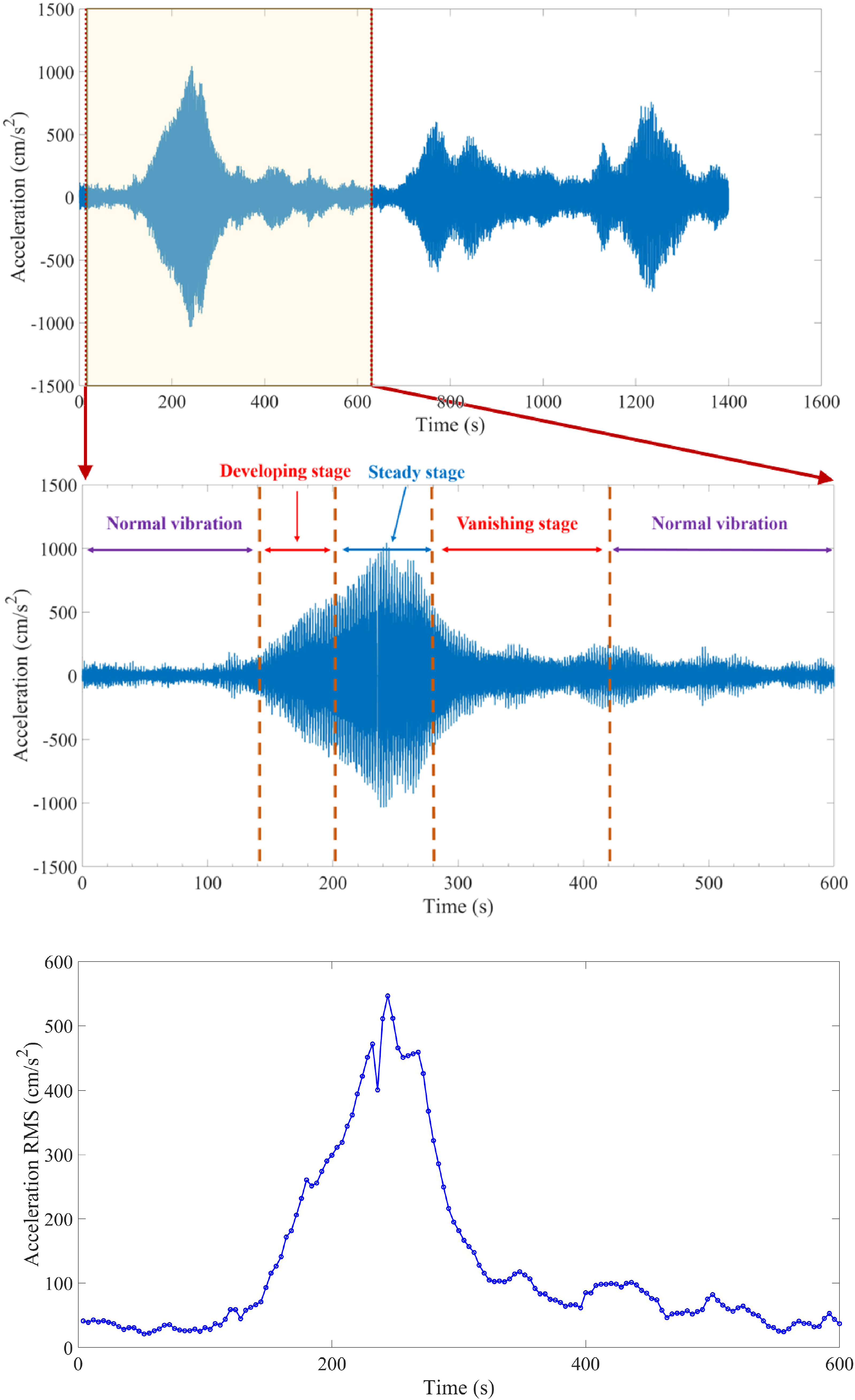
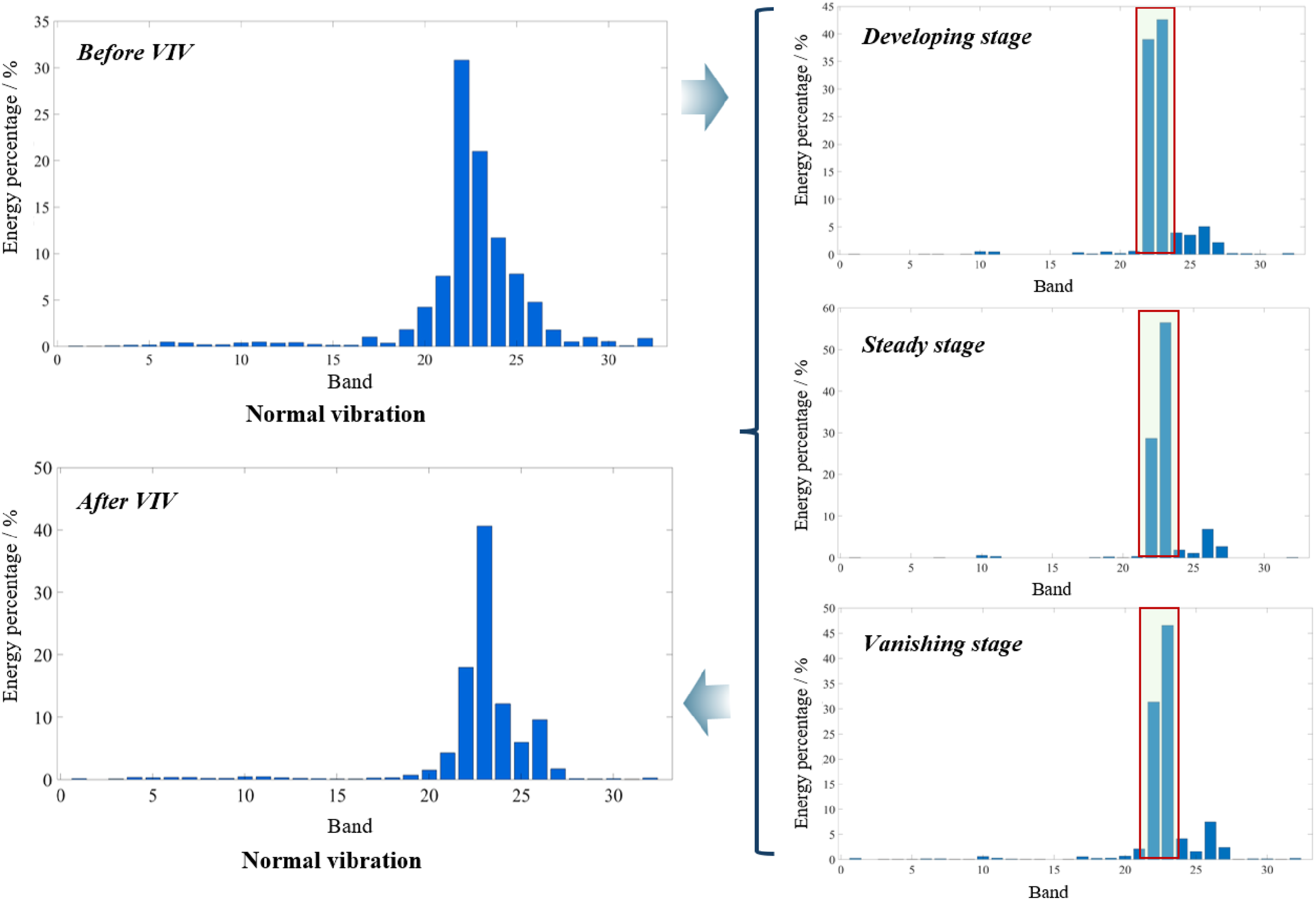
It can be observed from Figure 14(a) that the vanishing stage undergoes a prolonged period before gradually returning to normalcy instead of immediately transition into a state of normal vibrations. Comparing the time-domain amplitude with the wavelet packet energy distribution, it reveals that during the steady stage of VIV, the amplitude is exceptionally large with the corresponding wavelet packet energy proportion reaches peak. However, the amplitude during the developing and vanishing stage is not notably pronounced, which leads to vibrations fail to classified as VIV during the two stages in some cases. Despite the impact of the misclassification of VIV relatively modest, the cumulative energy still reaches approximately 80%, indicating that judging the occurrence and cessation of VIVs based solely on amplitude may not be sufficient. The accumulation and dissipation of energy in the stay cable system require a considerable amount of time. Once the energy in the stay cable system has not completely dissipated, there is a high likelihood of VIV recurrence, as illustrated in Figure 14. Therefore, the significant differences in energy distribution ratios revealed by wavelet packet decomposition between VIVs and normal vibrations were leveraged in this study. And the sum of energy proportion in adjacent frequency bands was used as a feature for DL classification, which could effectively distinguish VIVs of stay cable from other normal vibrations.
Proposed VIVs identification methodology for stayed cables
VIVs identification model for stay cables
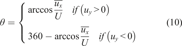
In this study, wind field characteristics including mean wind speed and direction at low and high height while dynamic characteristics including RMS and energy proportion, were taken as the feature input parameters of DL. The mean wind speed U and wind direction θ at low and high height with the10 min time interval can be calculated by following equations:


The RMS can be calculated by equation (12):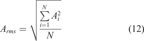
According to Figures 14 and 15, it can be seen when the stay cable is during the development stage of VIVs, the accumulated energy of the frequency band corresponding to VIV of the stay cable reaches 80% of the total energy, while the acceleration only reaches 500 cm/s2, which is far lower than that in the steady stage (1000 cm/s2). Therefore, based on the characteristics of differences in development stage, the RMS can be utilized as the hyperparameter to divide data into binary classification and label. The RMS value for classification and labeling is defined as the RMS feature threshold. Then using DL to effectively identify and classify.
Figure 16 presents the proposed VIVs identification framework of stay cables. To begin with, the monitoring data will be obtained through the SHM system, comprising real-time monitoring data and historical data. Subsequently, the RMS values from the feature library will be used as the basis for data classification, based on the RMS feature threshold, and automatic label classification will be performed. And the rest of the data from feature library will be utilized as DL training data set. Finally, the processed data will be input as the test set into the DL model for classification regression, which will constantly updated according to the evaluation and feedback of the identification results, resulting in the classification for VIVs. Diagram of VIV classification.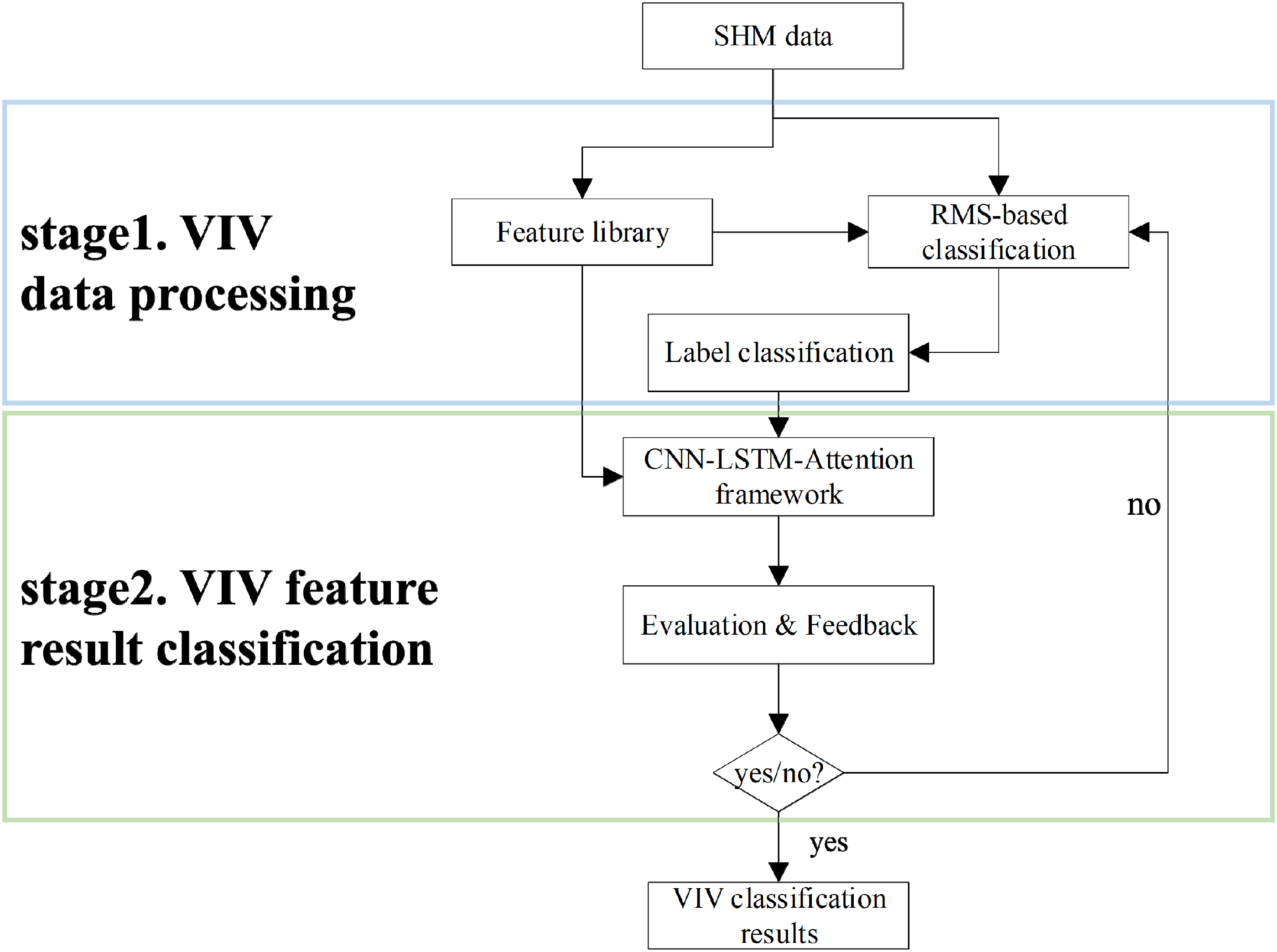
DNN framework design and result classification
In this section, a VIVs identification framework utilizing DL was established to facilitate the identification of VIVs in stay cables based on a large volume of field monitoring data. DL techniques overcome the limitations of shallow ML methods, such as limited expressive capability and low dimensionality, especially when dealing with large-scale datasets. Moreover, It also enables the joint optimization of feature extraction and pattern identification, conferring significant advantages in classifying extensive datasets (Z. Q. Chen et al., 2015).
Figure 17 illustrates a DL model combining CNN, LSTM and attention mechanism, which effectively combines the feature learning ability of CNN, the information memory ability of LSTM, and the attention mechanism improves the efficiency of the neural network. CNN is widely applied for the excellent feature learning capability (Y.-J. Cha et al., 2018), especially in the field of image recognition of crack detection (Zhao et al., 2024) and damage identification of bridge structures (Gu et al., 2024). CNN mainly consists of an input layer, convolutional layer, pooling layer, fully connected layer, and output layer. The principle of feature extraction in CNN involves the convolution kernel sliding over the feature data map to perform convolution operations, thereby extracting the data’s features. To reduce number of features and training parameters while mitigate overfitting, a pooling layer was applied for feature selection. The main purpose of the fully connected layer is to map the feature space calculated from the previous layers (such as convolutional and pooling layers) to the sample label space. Its advantage lies in reducing the impact of feature locations on the final classification result, and improving the overall robustness of the network. VIV identification process of cable-stayed cables based on CNN-LSTM-Attention.
After feature learning with CNN, it is necessary to classify or regress these features. As the depth of neural networks increases, the optimization function tends to get stuck in local optima rather than reaching the global optimum. LSTM networks (LSTMs) were introduced as an improved model to address the vanishing gradient or exploding gradient problems associated with Recurrent Neural Network. LSTMs are well-suited for handling sequential data structures (Wang et al., 2023), and are capable of effectively handling data with multiple coupled factors for prediction and recognition ((Feng et al., 2023; C. Wang et al., 2022; Wang et al., 2023). LSTM is composed of three gate units: forget gate, input gate, and output gate, which allow LSTMs to effectively capture and process sequential information. The forget gate, consisting of a Sigmoid activation function, selectively decides what information from the previous time step to forget. It can be expressed by equation (13). The information pass through the forget gate then move to the input gate C
t
, which is responsible for updating the current cell state. The input gate determines which pieces of information should be updated and passed to the hidden state h
t
.
To enhance the computational efficiency of the neural network, the attention mechanism was introduced, which dynamically allocates weights to different parts, allowing for a better capture of crucial information within the input data. The Attention mechanism firstly takes the input information, then calculates the attention distribution 
The specific operation process involves initially inputting the input features in a format that matches the convolutional kernel size into the convolutional network. There are 50 neurons, and a 2D convolutional layer is used. Rectified Linear Units (ReLU) are employed as the activation function in all hidden layers. After average pooling, the CNN network enters the sigmoid function for classification and proceeds to the flattening layer for data flattening. Subsequently, the data is input into the LSTM network for data prediction and classification, with the simultaneous utilization of the attention mechanism to enhance efficiency. Finally, it proceeds to the fully connected layer for data regression and output of results. The identification results are presented in the form of a confusion matrix in Figure 18. The confusion matrix describes the four regions of binary classification, which are True Negative (TN), False Negative (FN), False Positive (FP), and True Positive (TP). Confusion matrix prediction results diagram.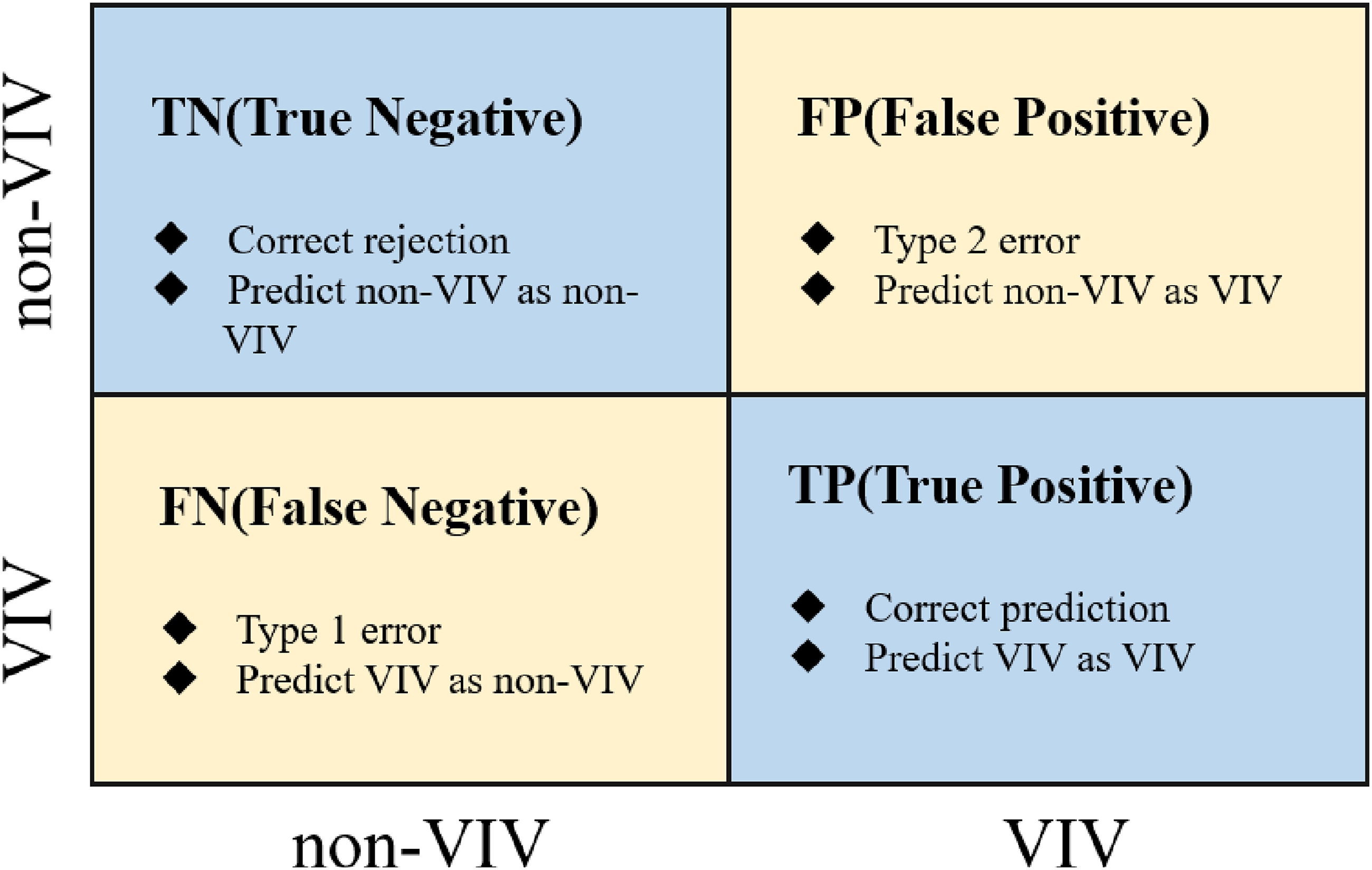
Vibration acceleration can effectively reflect the response characteristics of stay cables to VIVs during development stage of VIVs. Therefore, the relationship between the wavelet packet energy proportion and the RMS of acceleration in the identification results was presented. The identification results of the DL model under different RMS feature threshold classifications are shown in Figure 19, where blue, green, red, and purple represent TN, TP, FP, and FN, respectively. Lim et al. (2022) pointed out that FP results cover the development and vanishing stages of VIVs, which may lead to misclassification of non-VIVs as VIVs. The TP segment corresponds to the steady stage, while the FN segment represents abnormal vibrations similar to VIVs. According to the DL recognition results, the FP classification results increase with adjustments to the RMS feature threshold, indicating that the DL model can identify weak VIVs as VIVs within a large number of TN instances. DL identification results under different RMS feature thresholds.
When the acceleration RMS is in the range of 120 cm/s2 to 220 cm/s2, there is a significant amount of FN misclassification, mainly distributed near the decision boundary and in abnormal broadband large-amplitude vibrations with lower energy concentration. However, there is also a significant misclassification of normal steady-state VIV when RMS is in the range of 280 cm/s2 and 300 cm/s2, due to the high RMS classification threshold, many steady-state response stage VIV instances are classified as FP. Conversely, when the RMS reaches 260 cm/s2, the identification results are more accurate with fewer misclassifications, and the FN misclassifications are mainly low-energy abnormal vibrations.
Analysis of VIVs identification results
Identification results
In this study, field monitoring data of wind speed, wind direction, and acceleration for the stay cable were selected and organized. The data was segmented into training samples at 1 min interval. The identification of VIV involves the classification of 9420 data samples, and the identification results of the stay cable VIV based on the CNN-LSTM-Attention model are presented in Figure 20. Figure 21 illustrates the ambiguity in determining the decision boundary, which explains traditional threshold-based VIV identification is unreliable. On the contrary, the DL framework can enhance reliability by integrating a broader set of learning features, thereby producing more accurate identification results. VIVs identification results: confusion matrix. Identify the relationship between the ratio of energy proportion and the RMS of acceleration in the results.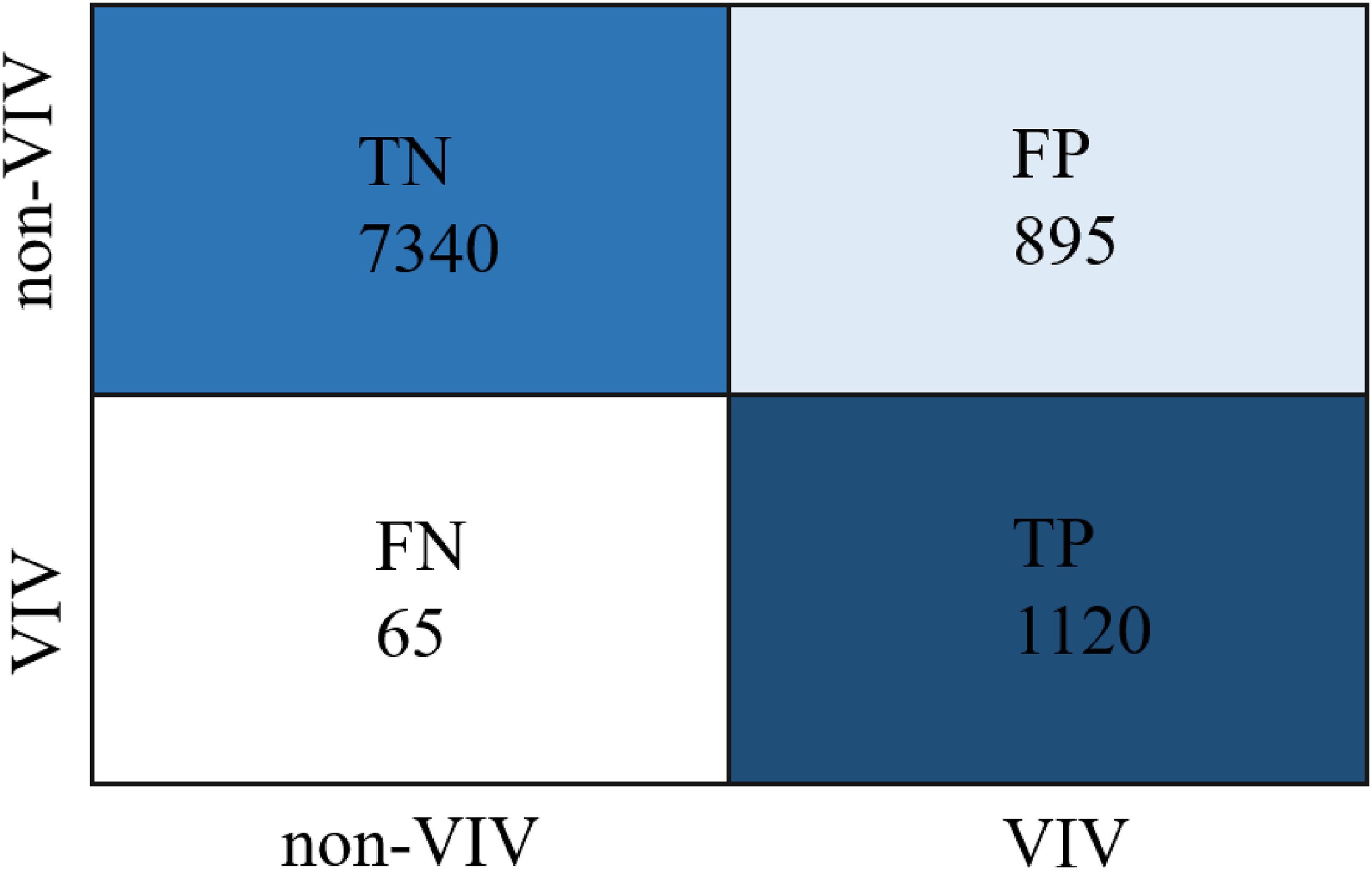
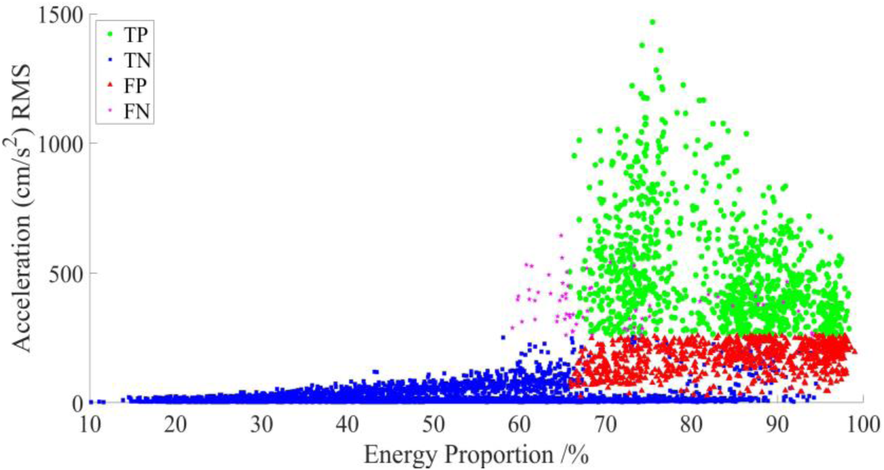
As shown in Figure 21, some anomalous identification results are located around an energy proportion of approximately 70%. Although some high-energy proportion true negative (TN) data might be indeterminate, comparing acceleration magnitudes suggests that it fails to pose a threat to structural safety.
Discussion of VIVs in different stages
To validate the accuracy of the identification results, two instances representing different stages of the VIV development process were selected for detailed analysis. Two instances covered scenarios of TP, TN, and FP, allowing for a comprehensive understanding of the relationship between the identification results and the actual occurrence of VIVs. As shown in Figure 22(a), wind speed and direction tended to reach a relatively stable state during the development of VIV. In Figures 22(b) and 23(b), the TP phase indicates that the amplitude is significantly larger than the normal vibration phase and remains relatively stable. Moreover, the amplitude is not a pure harmonic while a state where multiple harmonics coexist. By examining the frequency domain energy results in Figure 22(c) and 23(c), it is evident that TP phase represents a multi-modal VIV state. Identify result verification cases 1 (2010/7/10 17:01-17:20), (a) Mean wind speed and direction, (b) Acceleration time history, (c) STFT and PSD of TN, FP and TP, (d) Energy proportion of TN, FP, TP. Identify result verification cases 1 (2011/4/7 5:11-5:30), (a) Mean wind speed and direction, (b) Acceleration time history, (c) STFT and PSD of TP, FP, TN, (d) Energy proportion of TP, FP, TN.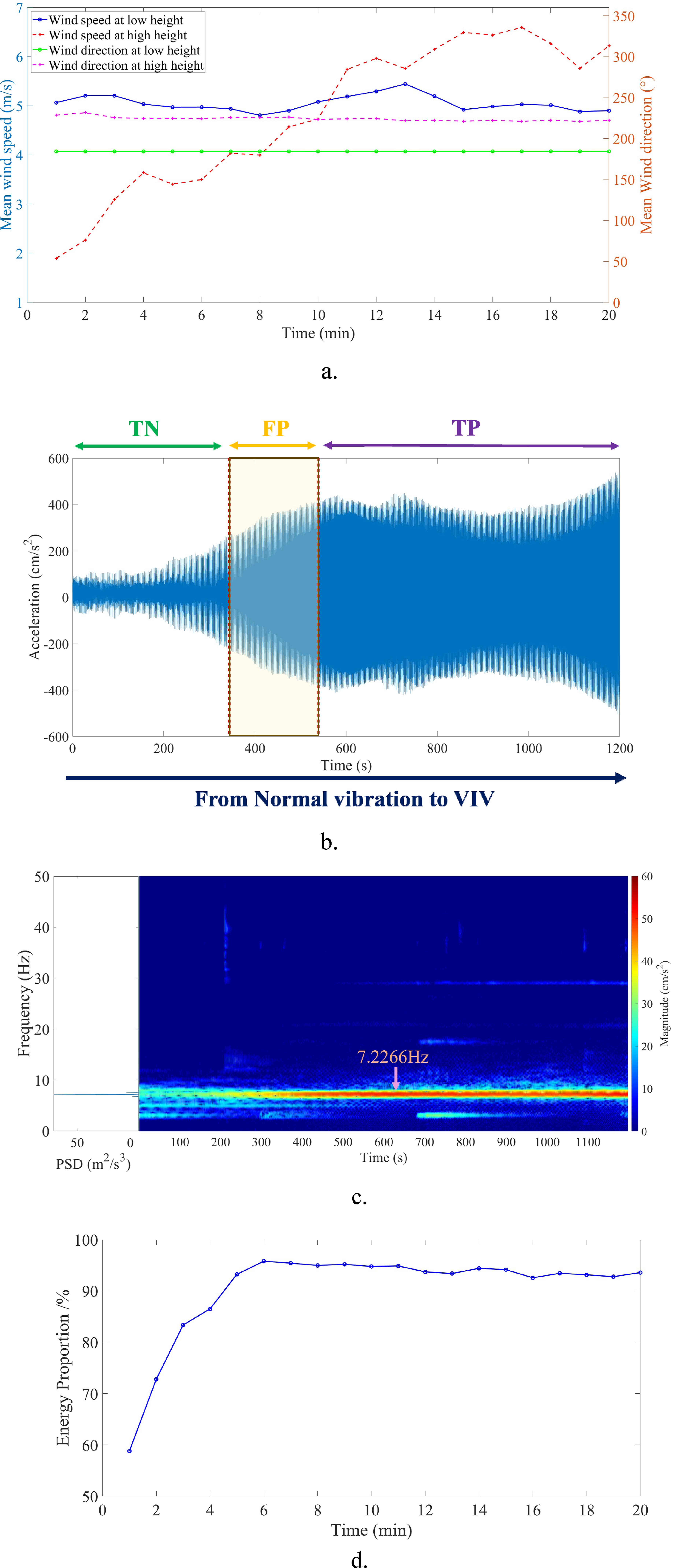
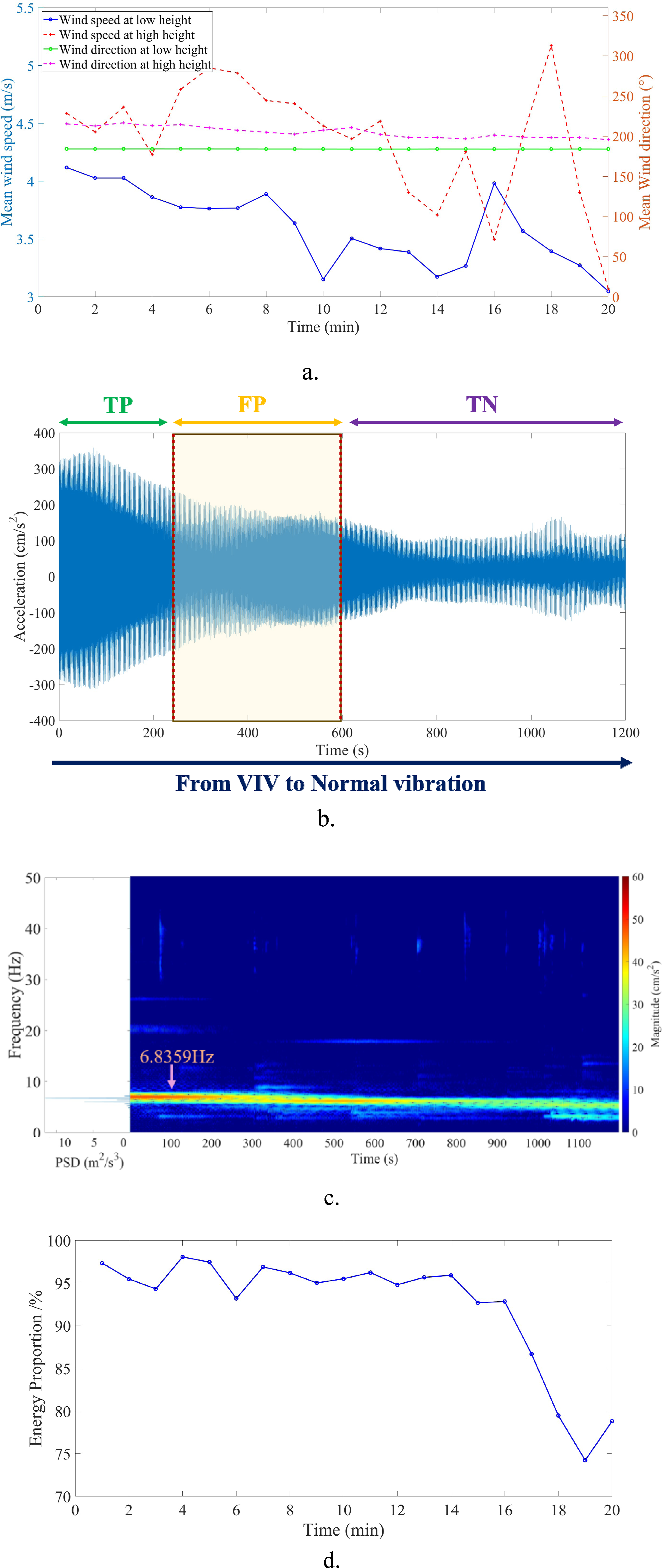
Simultaneously, it can be observed from FP phase stage that vibration amplitude significantly increased or decreased when VIVs were during the development and vanishing stages. Sample points were situated around the decision boundary, where traditional semi-supervised classification struggles to provide accurate results. The DL framework classified above sample points as FP, thereby enabling VIV warning. Figures 22(d) and 23(d) illustrate the distribution of wavelet packet proportion, indicating that when VIVs were during developing and vanishing stages, the energy corresponding to the VIV frequency band increased or decreased, which corresponds to the changes in energy magnitude over time of STFT in Figures 22(c) and 23(c).
It can be seen that VIV of the stay cable fail to dissipate immediately during the vanishing stage. On one hand, the threat of VIV is minimal due to the small acceleration amplitude. On the other hand, high-frequency vibration persists, resulting in the energy of the corresponding frequency band remains high (close to 80%). This is related to the low damping and high flexibility characteristics of the stay cable, indicating that a quick transition from VIV to normal vibration is challenging. Furthermore, it also suggested that the damping system of the stay cable exist defect.
Figure 24 presents the results of the FN classification, which indicate the abnormal vibrations during VIV. According to the frequency spectrum and wavelet packet energy proportion in Figure 24(b) and (c), the energy proportion across the frequency band is relatively broad, with frequent alternation of dominant modal frequencies. As analyzed in the acceleration time history in Figure 24(a), the beating vibration phenomenon under multi-modal coupling occurs. Due to the low damping of the stay cable and the dense modal frequencies, beating vibration easily occurs. It differs from the normal steady-state response of VIV, leading to anomalies in deep learning classification. Meanwhile, abnormal vibrations also exist around the decision boundary, which can be reduced by increasing the depth of the neural network and enhancing the training data. FN identification result, (a) Acceleration time history, (b) STFT and PSD of FN, (c) Energy proportion of FN.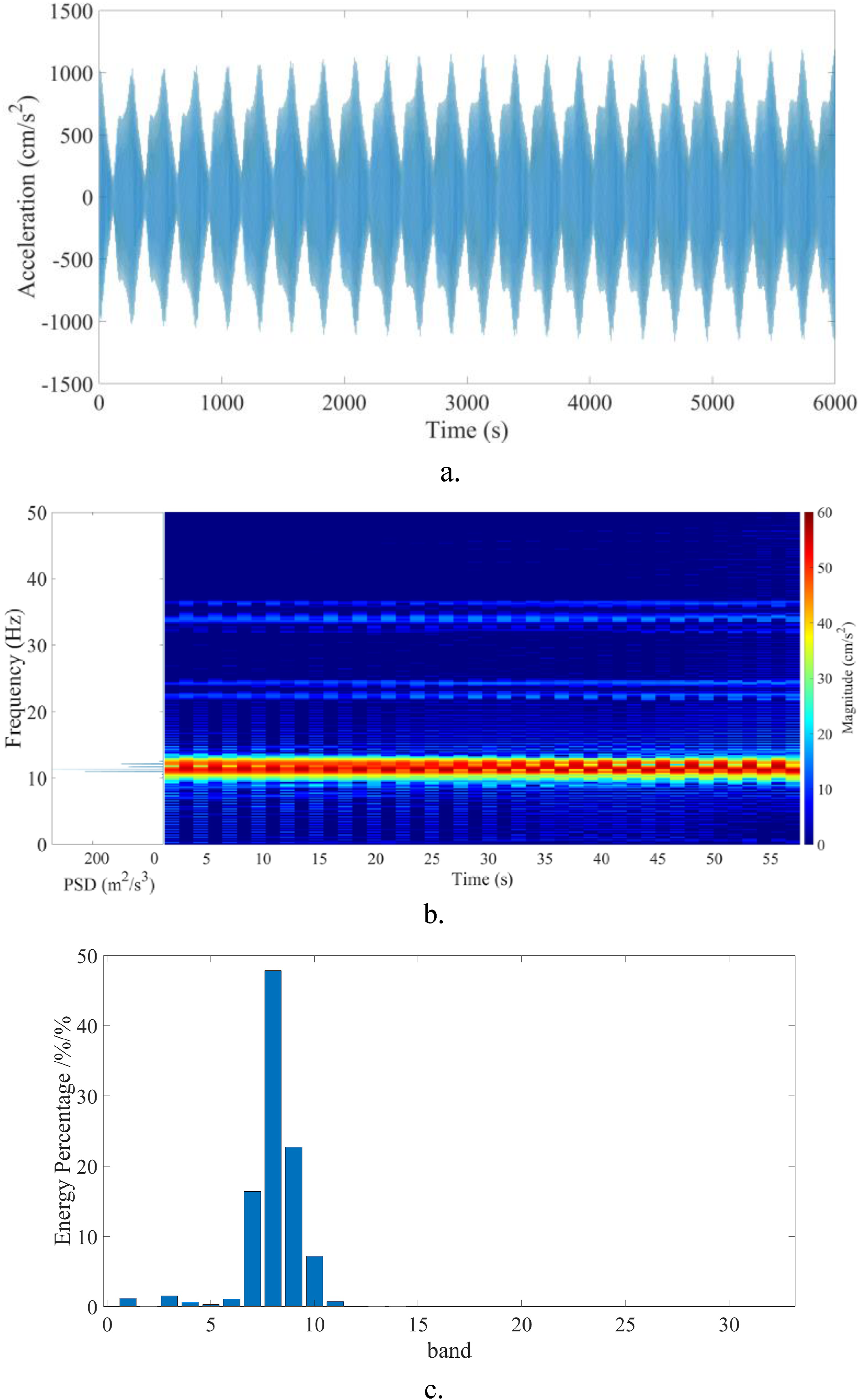
In this section, each classification in the confusion matrix of the identification results were discussed and validated. Then, two identification result instances and one anomalous classification were provided for verification and analysis, demonstrating the effectiveness and robustness of the VIV identification. Additionally, a comprehensive analysis of the FP and TP classifications was conducted. FP represents the development and vanishing stages of VIV, while TP represents the steady-state response. This capability not only can detect the steady-state response stage but also identifies the developing stage, serving as an early warning mechanism and thereby enhancing the identification of VIV in stay cables. Meanwhile, FN classification is identified as anomalous broadband vibration. Although a few misclassifications exist, it can be avoided with more data collected by SHM system and increased network depth.
Conclusion
Based on the foundation of field monitoring data collected by structural health monitoring system, this study conducted a validation of VIV data pertaining to a stay cable. The phenomenon of VIVs in stay cable was analyzed. Finally, a deep learning-based approach was employed to identify VIVs in the stay cable. The primary contribution of this study lies in distinguishing VIVs from the perspective of frequency domain energy distribution using the method of wavelet packet decomposition. The energy proportion coefficient was introduced as one of the characteristic indicators. By establishing a comprehensive identification process, real-time and automatic recognition of VIVs in stay cables can be achieved.
This study employs wavelet packet decomposition to visually represent the energy distribution of multi-mode VIVs in stay cables across different frequency bands. This approach effectively highlights the differences in energy distribution among these vibrations. When stay cables undergo multi-mode VIVs, the energy distribution typically manifests as the cumulative energy of adjacent frequency bands constituting more than 80% of the total energy, while the energy distribution of other vibrations tends to be more dispersed. This characteristic effectively distinguishes VIV from non-VIV. Furthermore, despite the restoration of normal acceleration, the energy in the frequency bands associated with VIV does not dissipate immediately.
A robust DL model was designed specifically for the identification of VIV in stay cables. The model utilized the differences in RMS and wavelet packet energy during the developing stage of VIV for appropriate label classification. Validation of the model was conducted based on the results of a confusion matrix. A detailed analysis was performed on two vibration instances to further scrutinize the identification results. Although the acceleration in TN instances is considerably lower compared to TP instances, it can be observed that the vibrations in TN instances are not entirely in a normal state. Despite the lower acceleration, high-frequency vibrations persist, maintaining elevated power spectral density and wavelet packet energy proportion. It indicates a defect in the damping system of the stay cable structure, which hinders the structure from quickly transitioning to a normal vibration state. Meanwhile, the classification of FP and FN was discussed, and the significance of FP classification was revealed, demonstrating the ability of model to identify VIV during both the developing and vanishing stages. It suggests that although other classification methods might categorize VIV instances as non-VIV, the trained DL model can still identify VIV events in these cases. Consequently, this feature can be utilized for real-time early warning during the developing stage of VIVs.
Footnotes
Author contributions
J.G.: original draft, Supervision, Methodology, Conceptualization.; R.M.: Investigation, Data curation, Methodology, Writing - original draft & editing; K.M.: Writing – review & editing, Investigation; D.C.: Writing – review & editing.
Declaration of conflicting interests
The authors declare that they have no known competing financial interests or personal relationships that could have appeared to influence.
Funding
The author(s) disclosed receipt of the following financial support for the research, authorship, and/or publication of this article: This research is supported by the National Natural Science Foundation of China Grant No. (U22A20231, 52078461).
