
Abstract
Identifying an impact load applied to structural systems and taking a prompt maintenance action is critical in structural health management. While various approaches have been investigated, this impact load identification is still a challenging task, considering associated high-level measurement requirements and sophisticated dynamic characteristics of uncertain structural systems. In addressing this challenge, we propose a novel impact load identification method based on a convolutional neural network (CNN) that incorporates the system model parameter uncertainties. This method aims to estimate the location, magnitude, and direction of an impact load using just one multi-axis accelerometer. While CNNs are powerful DL classifier models capable of mapping a structure’s response to input excitation, their effectiveness is frequently hindered by the scarcity of training data. In this study, we proposed to utilize a Physics-Based simulator to generate the necessary training dataset. Physics-based simulators show great performance in robotics, building energy management, and cooling systems and it can provide valuable training data. Consequently, a physics-based simulator for uncertain systems was developed to bridge the gap between simulated and actual structures and evaluated using uncertainty analysis. To validate the proposed method, both numerical and laboratory case studies have been conducted. The Physics-Based simulator demonstrated its ability to effectively train the CNN model, addressing uncertainty issues in model parameters. Moreover, the applicability of this method was tested by utilizing a single measurement point in different locations, showcasing its versatility and potential for real-world engineering applications.
Keywords
Introduction
As a sudden dynamic force of significant energy, an impact load applied to a structure can cause serious damage. Particularly, if the impact load is applied to a system beyond the design considerations, that is, at undesired locations with unexpected levels of high energy, the detrimental results can be catastrophic (Zhang et al., 2021). Immediate identification of such an impact event and taking prompt action is crucial in preventing further disaster. However, measuring such short-time and extremely localized impact forces is not straightforward unless a load transducer is placed at the impact force location. Even predicting the impact force locations is not practically possible due to the unpredictable characteristics of the force and the complexity of the structures. Covering the whole structure with numerous sensors may be an option, but this is not practical when considering the associated cost and challenges of sensor installation (Ferreira et al., 2022; Aygün and Cagri Gungor, 2011). Therefore, indirect approaches to identify the impact force using structural responses have been investigated.
One indirect approach, frequency-domain methods, has been explored to estimate the input force applied to a structure by multiplying the inverse of the frequency response function (FRF) with the structural output responses (Liu et al., 2021b). Various inversion techniques, including but not limited to direct inversion, least square approach, and modal coordinate transformation method, have been investigated to find the inverse of the FRF. However, these FRF inverse methods intrinsically suffer from ill-conditioned problems, with performances highly sensitive to numerical modeling accuracy and measurement noise (Liu and Shepard Jr., 2005). Regularization methods have been widely used to address the ill-posed nature of the problem and improve the accuracy and robustness of the results (Jiang et al., 2020b), such as Tikhonov regularization, truncated singular value decomposition, and the conjugate gradient method (Bouhamidi et al., 2011; Chen et al., 2018, 2019). However, these methods require a well-chosen optimal parameter for accurate estimation of the input forces (Allen and Carne, 2008). Additionally, while the FRF-based method is more applicable to stationary conditions, it is not suitable for transient excitations, such as impact loads (Liu et al., 2021b).
Another indirect approach, time-domain methods, uses the kinetic equations of the structure to estimate the input forces from the output responses (Liu et al., 2016). Such time-domain methods include the coordinate transformation method (Desanghere, 1985), Sum of Weighted Accelerations Technique (SWAT), Inverse Structural Filter (ISF), and multi-step inverse structural filter (Allen and Carne, 2006). The coordinate transformation method transforms the system model, i.e., the equation of motion of the system, into modal coordinates (Briggs and Tse, 1992). This technique uses acceleration responses to estimate the force, but it can also be ill-conditioned (Briggs and Tse, 1992). The ISF method identifies the input force by inverting the state space representation (Allen and Carne, 2006). SWAT uses the idea of a modal filter to obtain rigid body accelerations and multiplies it by the mass properties to estimate the input forces and moments acting on the body’s center of gravity (Allen and Carne, 2006). However, the ISF method has suffered from stability issues, and the requirement of a large number of sensors for SWAT limits the use of the method in real practice (Allen and Carne, 2006). Different regularization methods have been used to solve the issue with inverting the direct equation for impact load (Liu et al., 2023; Zhou et al., 2024c). However, uncertainties associated with model parameters can affect the accuracy of identifying the load (Zhou et al., 2024b).
Statistical methods have been investigated to account for such uncertainties in system modeling and sensor measurement (Liu et al., 2018). These statistical methods include PDF-based algorithms, Bayesian formulations, and the Kalman filter (Jiang et al., 2020a; Li et al., 2021; Saleem and Jo, 2018; Yan et al., 2017). However, the uncertainty levels and system sizes that these methods can consider are quite limited (Liu et al., 2021b), and the performances of the methods heavily rely on the number of sensor measurements used in the process (Saleem and Jo, 2018).
As a data-driven approach that can establish a connection between data or features and a desired output (Müller and Guido, 2016), Machine Learning (ML) has demonstrated significant success in civil engineering applications, including but not limited to structural design (Sun et al., 2021), load identification (Cao et al., 1998a; Liu et al., 2022; Yang et al., 2021; Zhou et al., 2019), geotechnical engineering (Ahmad et al., 2007; Bagińska and Srokosz, 2019), and damage detection (Avci et al., 2021; Mehrjoo et al., 2008; Padil et al., 2020; Pawar et al., 2007). In recent years, various ML algorithms have been employed to identify input loads on structures, such as Artificial Neural Networks (ANN), Recurrent Neural Networks (RNN), and Support Vector Regression (SVR). ANN has been applied to identify input loads using strain measurements on cantilevered beams (Cao et al., 1998b), determine the locations and magnitudes of impact forces on plates (Sung et al., 2000; Worden and Staszewski, 2000), and reconstruct dynamic loads with uncertainty (Liu et al., 2022). However, ANN methods require many learnable parameters, leading to computational challenges and potential overfitting issues Ismail Fawaz et al. (2019). Long Short-Term Memory (LSTM) and Bidirectional Long Short-Term Memory (BLSTM), developed to address gradient blow-up or disappearance in RNN, are used for finding patterns in sequences of data, making them suitable for time series analysis (Schmidt, 2019). LSTM and BLSTM have been utilized to identify dynamic loads on beams (Yang et al., 2021) and impact loads in nonlinear structures (Zhou et al., 2019), yet they require high computational power and can be challenging to train (Liu et al., 2019). Support Vector Regression (SVR) is a supervised machine learning technique for solving regression problems (Mechelli and Vieira, 2019). SVR constructs a regression formula that maps the observed variable to the target output (Mechelli and Vieira, 2019). Zhang and O’Donnell used SVR to identify dynamic loads with interval uncertainties using heterogeneous responses (Liu et al., 2021c).
The Convolutional Neural Network (CNN) is a deep learning (DL) method that uses convolutional and pooling layers to classify and extract features simultaneously (Zhao et al., 2017). The main advantage of CNN is feature extraction, where raw data can be used directly without the need for human interference (Zhao et al., 2017). Moreover, CNN has the capability to extract features that are not visible to humans and choose patterns to maximize the model’s accuracy. While CNN is commonly used in analyzing visual data or two-dimensional data such as image classification, it has also shown great performance in analyzing noisy time series data and can learn high-level patterns (Zhao et al., 2017). In recent years, CNN has been used in crack detection (Cha et al., 2017; Chen and Jahanshahi, 2017), damage detection (Duan et al., 2019; Xu et al., 2019), and system identification (Wu and Jahanshahi, 2019). Moreover, Yang et al. (2023) was able to identify dynamic loads using CNN with uncertain model parameters and Zhou et al. (2024b) developed an impact force localization and reconstruction method using a gated temporal convolutional network.
While these ML methods have shown great potential in dynamic load identification, they suffer from two main limitations. The first is the lack of data to train the ML models (Talaei Khoei et al., 2023; Vadyala et al., 2022a). Training data can be collected either numerically or experimentally (Sung et al., 2000; Talaei Khoei et al., 2023; Yang et al., 2021). However, extracting training data experimentally from the field is a challenging task (Agdas et al., 2016a). Several efforts have been made to integrate ML and DL methods with physics-based models in the loss function to improve the generalization of ML and DL models and reduce data dependency for civil engineering applications (Vadyala et al., 2022b), such as load identification (Zhou et al., 2024a). However, experimental data is still needed for training. Generating training data numerically can be an alternative way, where the laws of physics are used to simulate the dynamic system input and output. This approach, often referred to as a physics-based simulator, leverages fundamental principles and equations governing the behavior of systems to create synthetic datasets (Liu and Negrut, 2021). The combination of Physics-Based Simulators and ML models has been applied in various applications, such as building energy management and cooling systems (De Wilde et al., 2013; Xuemei et al., 2009; Yun et al., 2012), as well as robotics (Liu and Negrut, 2021). Physics-Based Simulators can generate a large amount of training data in a short period and provide the necessary training events for ML models (Liu and Negrut, 2021). While this technique leverages the benefits of both Physics-Based and ML approaches, it is essential to have an accurate Physics-Based model. However, uncertainties associated with system model parameters (i.e., material properties), machining errors, and signal noise (Liu et al., 2021c, 2022) can reduce the accuracy of the Physics-Based model and lead to the creation of unrealistic data (Liu and Negrut, 2021).
Various algorithms have been developed to address the issue of uncertain systems for dynamic load identification (Liu et al., 2021c, 2022). In these methods, a large number of measurement points and displacement measurements were used to identify the load, which introduces the second issue of dynamic load identification methods. Increasing the number of measurement points will result in increased associated cost and complexity of the sensing system and consequently limit practical use (Agdas et al., 2016a; Vadyala et al., 2022a). This is especially relevant in the context of bridges, where stringers/multi-beams or girders constitute the predominant structural systems (Farhey, 2018), and an increased number of sensors per girder increases the overall complexity of the monitoring system.
In this study, we developed a novel method for identifying impact loads using a minimal sensor setup, specifically utilizing a single sensor node. This approach is particularly advantageous in bridge engineering, where the structural framework predominantly consists of stringers, multi-beams, or girders (Farhey, 2018). Employing a single sensor per beam enhances the practicality of this method, which has been validated experimentally using a beam model.
The core of this method is a Convolutional Neural Network (CNN) model designed to accurately ascertain the location, direction, and magnitude of impact loads. Training of the CNN model is accomplished through a Physics-Based Simulator, which incorporates uncertainty to reflect real-world conditions. Given the novelty of employing this simulator for dynamic load identification, we devised a new technique to demonstrate its application in identifying impacts. To ensure the model’s applicability to actual scenarios, uncertainty is deliberately integrated into the simulation process. This aspect is crucial for mimicking real-world complexities and is extensively evaluated through a sensitivity analysis. Finally, the method’s performance is first rigorously validated through numerical analysis. Following this, it undergoes experimental testing to thoroughly evaluate its effectiveness.
Load identification problem
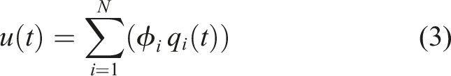
The response of a multi-degree-of-freedom dynamic system can be expressed as:

where

where
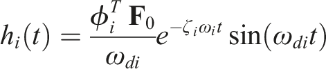
If the dynamic system is assumed to be linear and exhibits proportional damping, the differential equation (Craig and Kurdila, 2011) can be represented in modal coordinates as follows:

where q
i
is the modal coordinate and defined as:
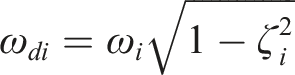
And ω
i
and ζ
i
are the natural frequency and damping ratio respectively, and

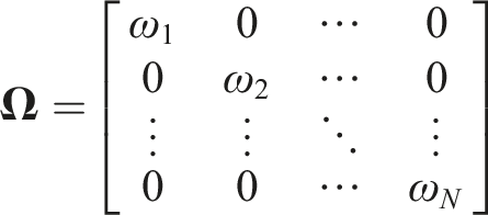


Let:

Then the modal equations become:

To find q
i
for any
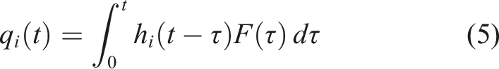
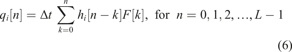
where L is the number of time steps and Δt is the time interval. The matrix form of Equation 6 is then given by:

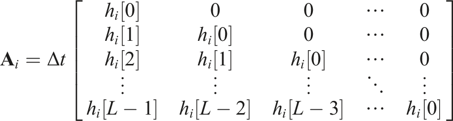


If:
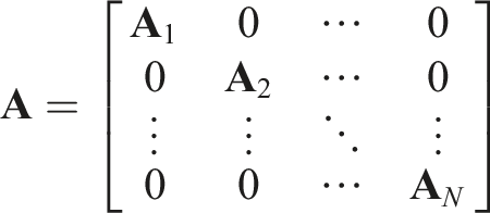
where each

From Equations 3 and 7:


And:

Where
To solve for

The accuracy of
To address these challenges, this study explores the potential of neural network methods in identifying the load applied to structural systems, with a focus on impact load identification. This study establishes a relationship between the measured dynamic responses and the impact load. In particular, the possibility of using only single-node acceleration responses as an input, in conjunction with CNN, for impact load location, magnitude, and direction identification for a whole structural system is explored, considering the uncertainties of the model parameters.
Impact load identification convolutional neural network method
In this section, the overall methodology of impact load identification using a CNN-based model that takes the acceleration response of the structure as input to estimate the location, magnitude, and attack angle of the impact load is described. Particularly, the model takes input from a single-node multi-axis accelerometer placed at a specific (i.e., optimal) location in the structure. Three CNN architectures are considered for three different tasks. The first task is to find the location of the impact load, the second one is to determine the magnitude, and the last one is to estimate the attack angle of the impact load.
Convolutional neural network
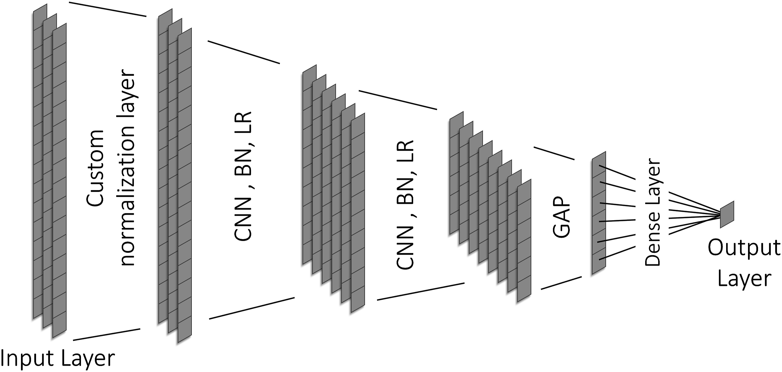
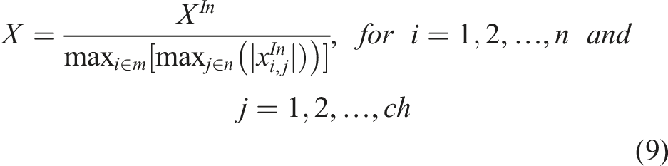
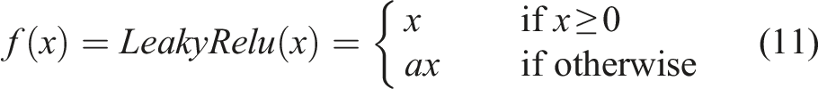
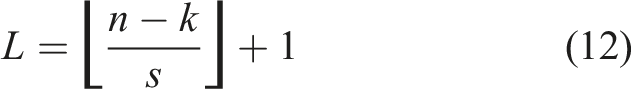
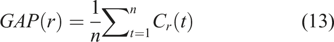
CNN, or Convolutional Neural Network, is a DL method that employs both convolutional and pooling layers to simultaneously classify and extract specific features from data, as illustrated in Figure 1. In the context of this study, either single or multi-axis acceleration responses are utilized as input to the CNN model to identify impact loads across multiple layers. The types of layers used in this study are described as follows: 1. Input layer - As described before, the model uses acceleration responses of the structure to identify the impact input force. As a result, a one-dimensional input layer is used with single or multi-channels that present the node acceleration response in different axes at a specific location in the structure. 2. Custom normalization layer - This layer is used right after the input layer to normalize the input signal for the location and angle identification tasks. In these tasks, the main objective of this normalization layer is to reduce the magnitude effect of the impact load and only focus on the location and angle features of the input force, as seen in Appendix A. 3. Convolutional layer - A one-dimensional convolutional layer with several one-dimensional filters or kernels is used to extract features from the acceleration signal. The filters have a dimension size of ch × k, where ch is the number of channels from the previous layer and k denotes the length of the filter. The filters slide through the time series with fixed strides to convolve them into features. A nonlinear activation function is used to determine the output of this layer. In this study, a LeakyReLU (LR) activation function is used. 4. Batch normalization (BN) - This layer is used to speed up the training process, allowing for higher learning rates, and improving generalization (Ioffe and Szegedy, 2015). The difference between BN and the custom normalization layer is that the custom normalization layer normalizes each response as seen in Equation 9 while BN normalizes the whole batch. The details of BN can be found in Ioffe and Szegedy (2015). 5. Global Average Pooling (GAP) - This layer is used to reduce overfitting by averaging the dimensionality of the features from the preceding layer into a one-dimension feature map. 6. Output layer - This layer has n number of neurons, where n represents the number of desired outputs, and the output layer is connected to the previous layer (i.e., GAP) through a transformation function. For classification operations, each neuron represents the probability of each class using the SoftMax activation function. For regression operations, a single neuron in the output layer directly computes the objective, such as the magnitude of the impact force. The overview CNN architecture.
Training convolutional neural network procedure
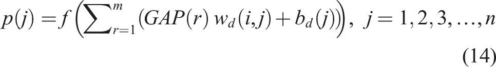
The CNN training procedure is composed of the following steps: The first step of the training procedure is to determine the CNN architecture. The general architecture of the proposed CNN model consists of the input layer, custom normalization layer, several convolutional layers with batch normalization (BN) and LR, global average pooling (GAP), and output layer, as seen in Figure 1. After building the CNN model, the weights and biases are initialized using the Glorot uniform initializer. Then, a learning rate (η) and the number of epochs need to be selected, along with an activation function for the output layer. The second step is to find the output of the CNN model using several layers, as described below: (a) Input Layer – This layer serves as the entry point to the neural network. The input shape of each response in the batch of the CNN model is (b) Custom normalization layer – As mentioned above, this layer is only used in location and angle identification tasks. This custom layer is defined as: (c) Convolutional layer – Equation 10 below describes the output of the convolution layer: (d) GAP layer - The output of the GAP: (e) Output layer - The output layer can be written as: 3. The last step is to update the weights and biases by minimizing the loss function using the Adam algorithm. The loss function is a function that determines the error between the desired output and the CNN output. Three types of loss functions are used in this study as discussed in the following sub-section. For more information on the Adam algorithm, please refer to Jiang et al. (2020a).

Convolutional neural network model for impact load identification
As mentioned above, three different tasks have been conducted to find the location, direction, and magnitude of the impact load, respectively. Identifying the impact load’s location should be the first task and is imperative in this study. Then, estimating its magnitude and direction follows. For determining the load’s magnitude and direction, a unique CNN model is designated for all potential impact locations within the structural system to enhance method accuracy. Each location has a specific CNN model trained exclusively for that particular location to estimate the magnitude and direction (i.e., tasks 2 and 3) of the impact load more accurately. The input of each CNN model is the acceleration response time history from a single sensor node affixed to the structure. In the following section, the architecture of the CNN for each task is described, and an overview of the proposed method is shown in Figure 2. The procedure of CNN-based impact load identification method. ch is the number of channel or measurement axis and n is the number of time sample.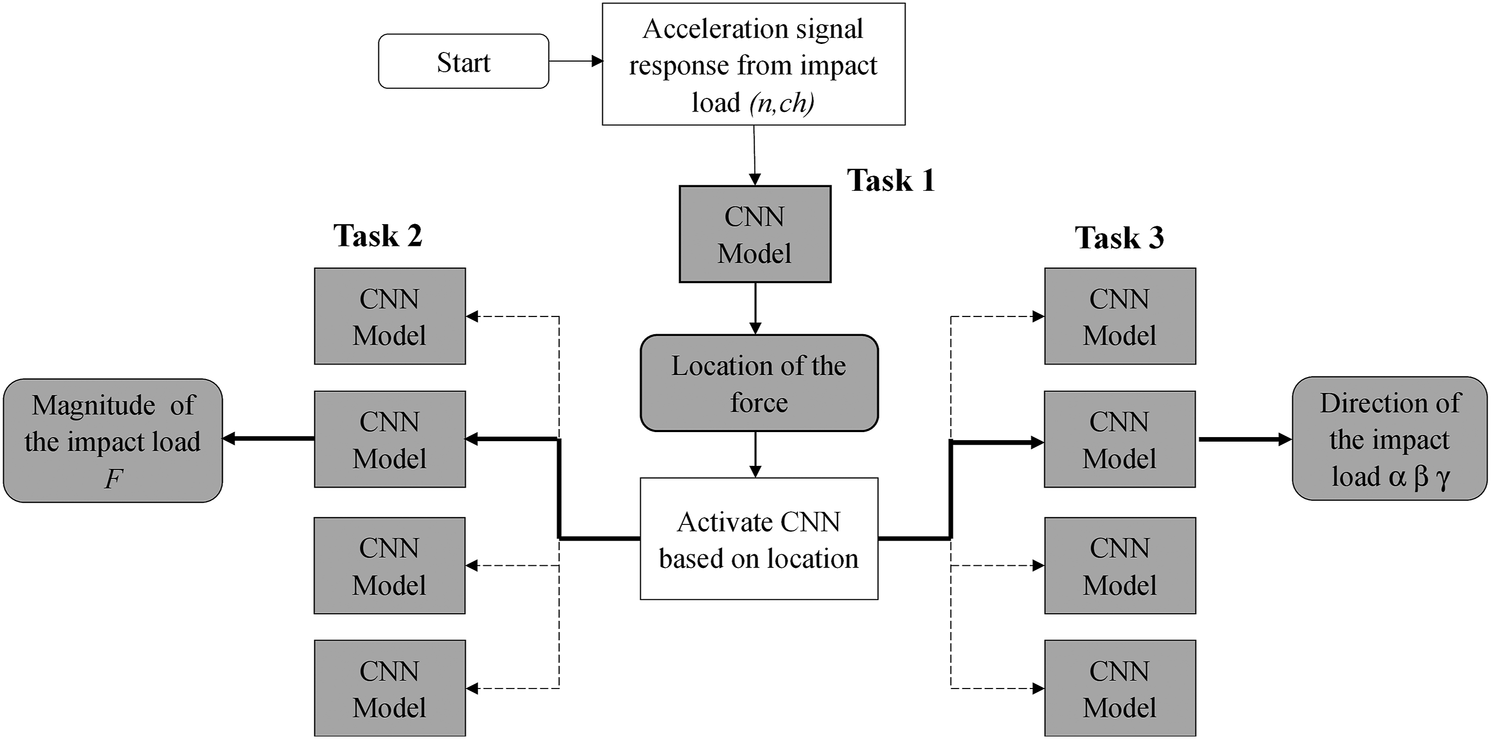
Task 1 - Location identification
The architecture of this CNN for location identification consists of the following components: an input layer, a custom normalization layer, several 1D convolutional layers, batch normalization layers between each convolutional layer, a 1D Global Average Pooling layer, and an output layer. As mentioned in the training CNN procedure sub-section, the custom normalization layer is used in this task because the objective is location identification. Therefore, each possible location and direction of the impact load should be included in the training set.
For the activation function of the output layer in this task, SoftMax is used:
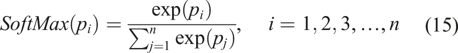
Where p is the output of the output layer, and n is the number of outputs.
For the loss function in this task, the categorical cross-entropy loss function is used, which is typically used for optimizing the CNN model for classification:

Where
Task 2 - Magnitude identification
After finding the location of the impact load, the designated CNN model for that location is assigned. The architecture of the CNN includes an input layer, several 1D convolutional layers, batch normalization layers between each convolutional layer, a 1D Global Average Pooling layer, and an output layer. For the activation function of the output layer in this task, a linear activation function is used:

Where p is the output of the output layer, and n is the number of outputs.
For the loss function in this task, a mean absolute error loss function is used, which has been typically used for regression estimation:
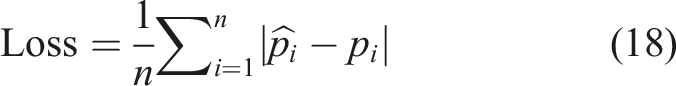
Where
Task 3 - Direction identification
In this study, a three-angle system was used to define the direction of the force in space. For example, a vector 3D vector in space representation using (a) two-angle system and (b) three-angle system.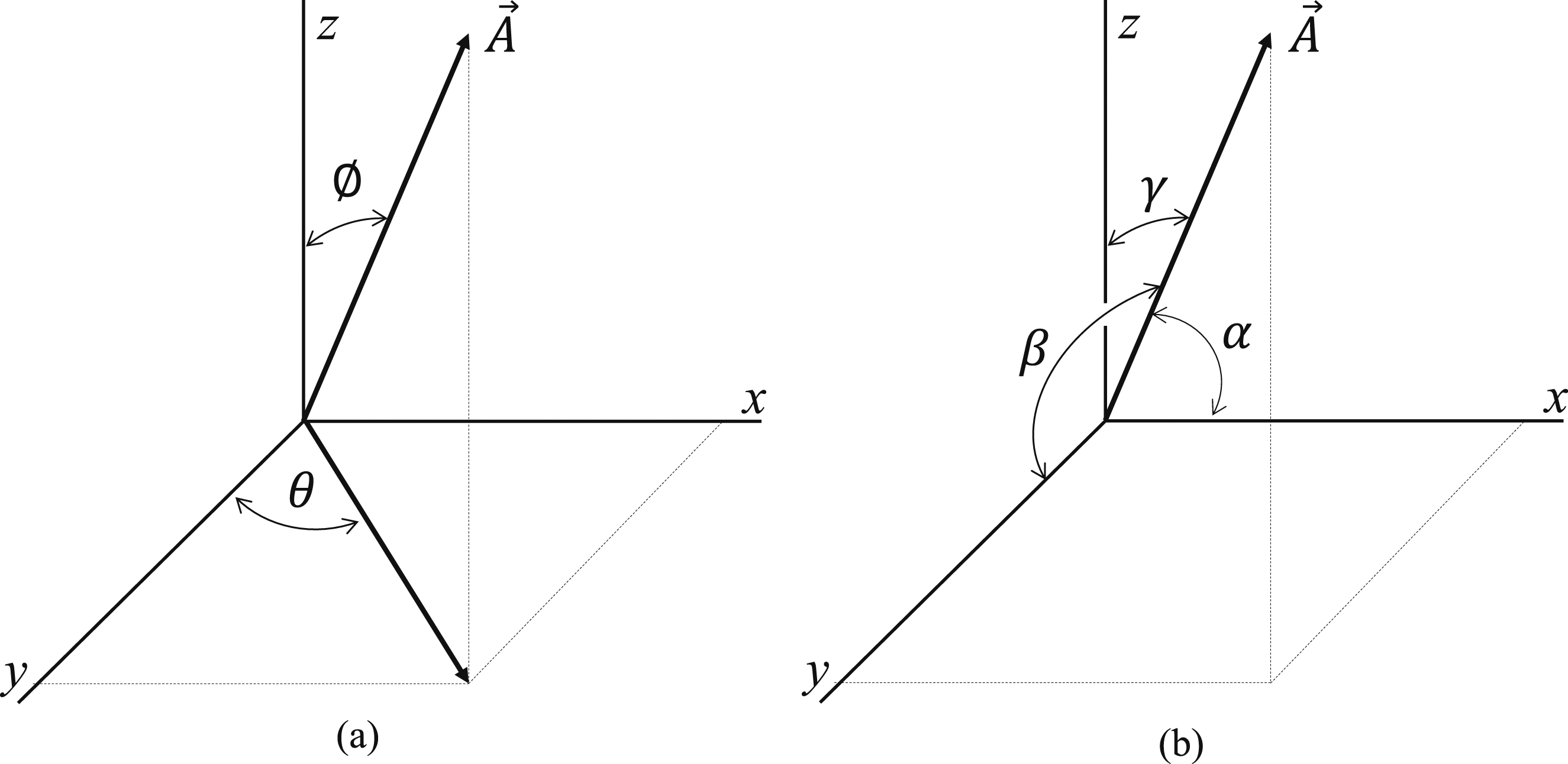

Where:
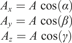
Where α, β, and γ are measured between the tail of

The number of outputs for this task is three, representing α, β, and γ. However, it is imperative that the estimated angles satisfy Equation 20. To meet this requirement, a custom activation function has been created:
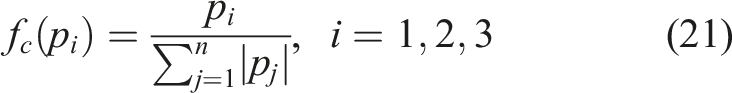
From Equation 21, the summation of the absolute value of the output always equal to one, so the output of the activation layer represent:
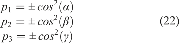
Where ± indicates that each p i can take either a positive or negative value. The specific sign of each p i will be determined by the CNN model.
To determine α, β, and γ, we employ the inverse cosine function:
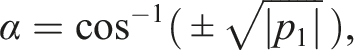
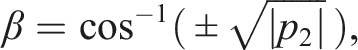

Where the ± sign is consistent with the sign of each corresponding
To generate the training data using numerical analysis, a two-angle system involving ϕ and θ was employed, as seen in Figure 3(b). The ϕ represents the angle between the impact load direction and the positive z-axis, ranging from 0 to 180°. The θ measures the angle in the x y-plane from the positive x-axis, ranging from 0 to 360°, measured counterclockwise. The relationship between ϕ and θ and the α, β, and γ is provided in Equation 23. This relationship ensures that the condition of Equation 20 is holds true for all generated directions.

Physics-based simulator with uncertainty
The equation of motion (Equation 1) can be expressed in a continuous state space form as below (Law et al., 2005):

Where:
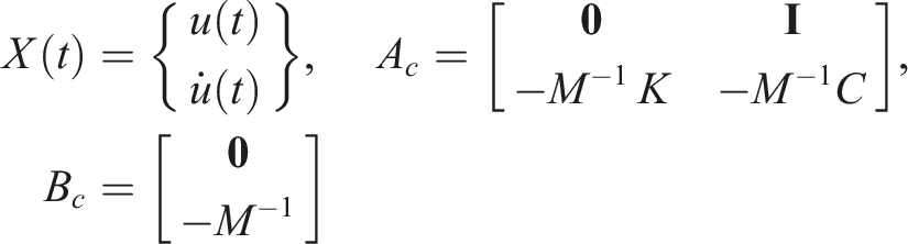
And:

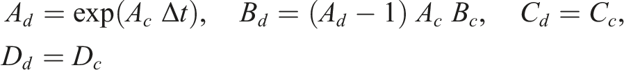
A discrete version of the state space formulation can be written below, which is used to generate the required data for training and testing the CNN models in this study (Law et al., 2005).
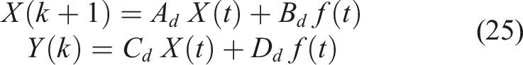
Where:
To account for possible uncertainties associated to the model parameters, the modulus of elasticity, mass density and damping ratio of the system model are set to be random variables and Equation 1 can be transformed into:

Where The procedure of the physics-based simulator.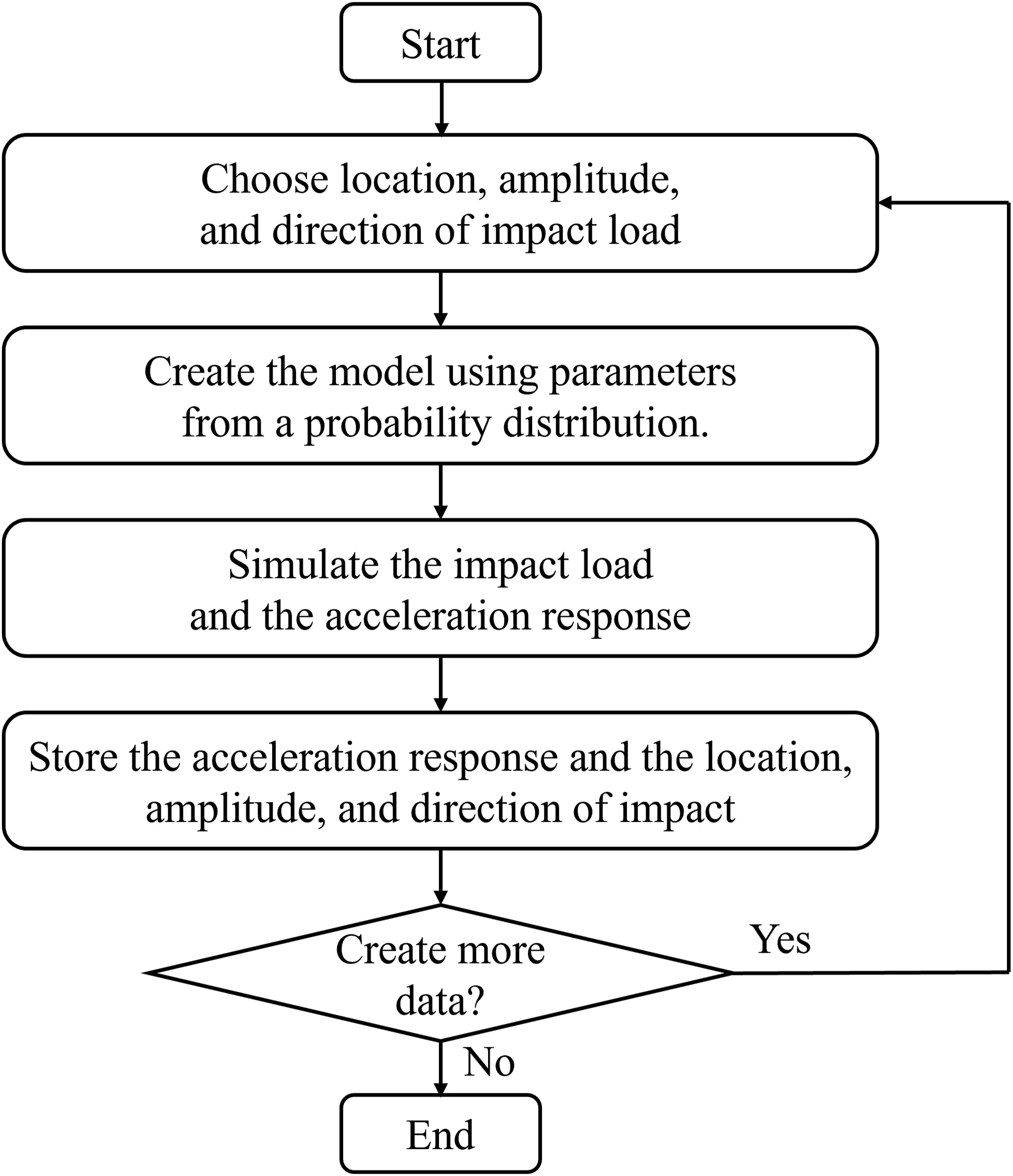
Considering modulus of elasticity, mass density, and damping ratio as uncertain parameters is sufficient to alter the overall mass, stiffness, and damping matrices in various structural dynamics scenarios, such as beam frames and trusses (Mario and Young, 2019). These structural elements are widely used in structural analysis and design (Lallotra and Singhal, 2017). In complex structures, these parameters interact intricately, necessitating detailed modeling to ensure accurate predictions of structural behavior. Additionally, boundary conditions, functional forms, variable definitions, equations, assumptions, and mathematical algorithms should be carefully considered while simulating the structure (Simoen et al., 2015; Walker et al., 2003). However, these factors required a specific structure to be identified.
Numerical case study
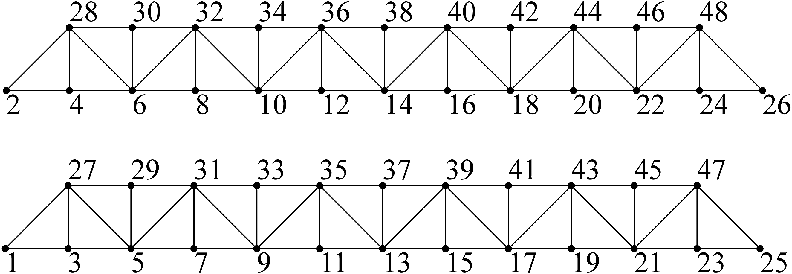
A numerical 3D pin-supported truss model is developed to test the performance of the proposed method. The truss contains 136 members and 48 nodes and is made from steel with a modulus of elasticity of 200 GPa, a constant cross-section having an area of 37.3 mm2, and a damping ratio of 2%. The truss is 4.5 m long and 0.61 m wide, as shown in Figure 5 and Figure 6. Geometry of truss structure. Truss side view and nods numbers.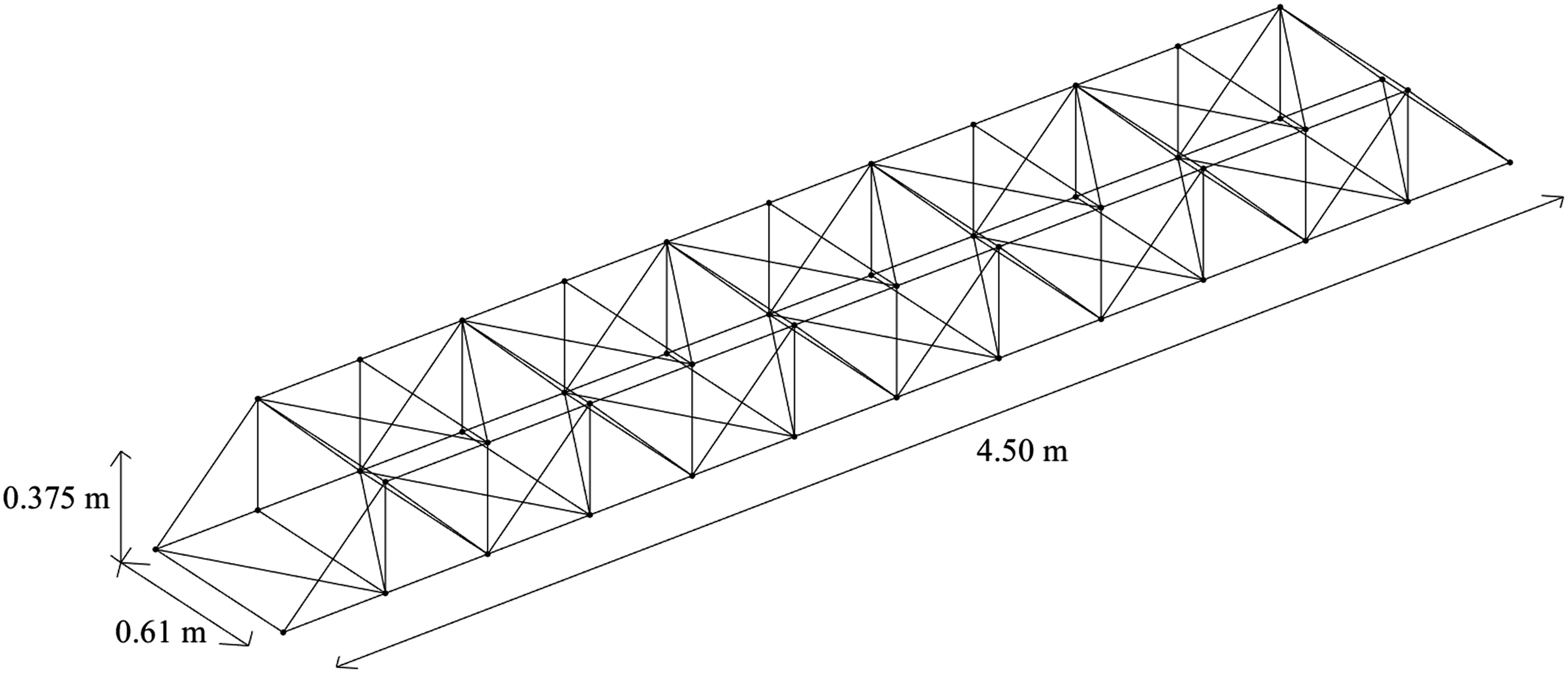
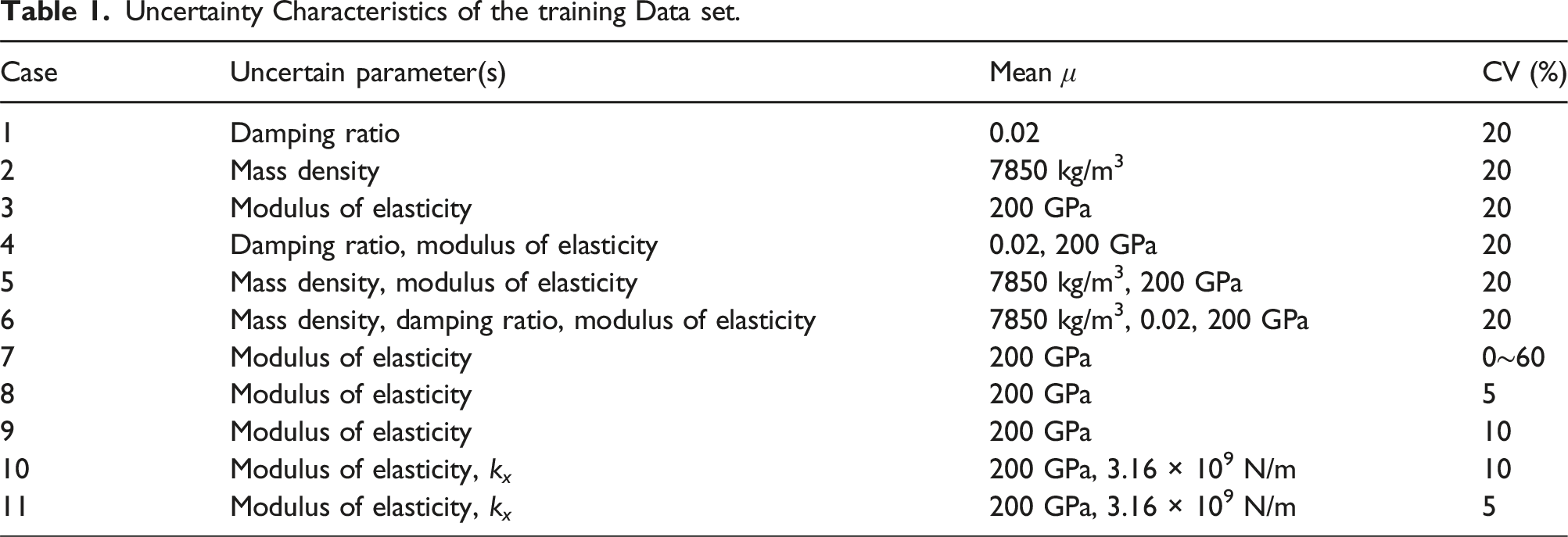
Uncertainty Characteristics of the training Data set.
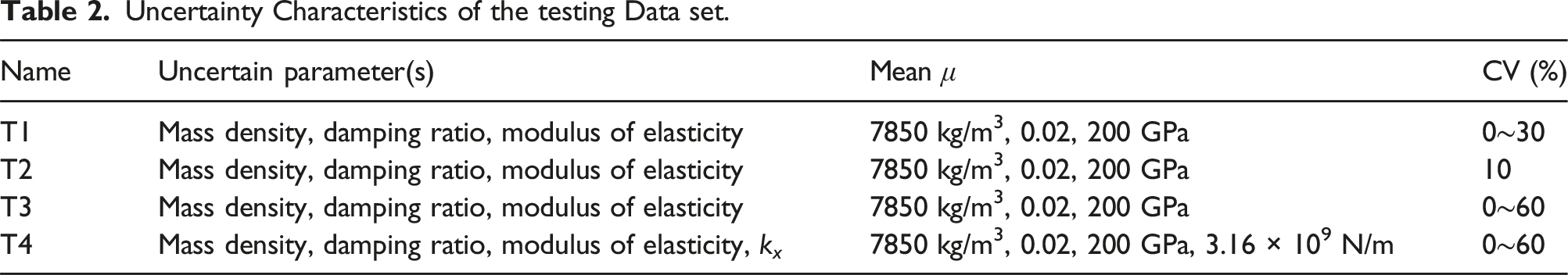
Uncertainty Characteristics of the testing Data set.
Task 1 - Impact load location identification
The truss has 44 possible impact locations (3 to 24 and 27 to 48 nodes) with different magnitudes and attack directions. To identify the location of the impact load. A specific CNN model for location identification was created, and the layer depth was determined and examined as seen in the sub-section on the effect of different architectures and hyperparameters. In addition, single-sourced and multi-sourced uncertainty cases were considered in the training and testing datasets to check the parameter uncertainty effect in the proposed method. The selection of impact load magnitudes and attack directions for the training and testing dataset is described as follows: • Training set: In every 44 possible location, the impact load directions were set to be between 0 and 180° for ϕ and 0 to 360° for θ, stepped by 10° for both angles. Additionally, for each direction, three different magnitudes of the impact load—5 N, 40 N, and 80 N—were applied, covering a range of impact forces. This setup generates a total of 83,172 datasets for training, covering a comprehensive range of impact scenarios across all locations, directions, and magnitudes. • Testing set: A dataset of 30,000 samples was created with uniformly random locations, directions, and magnitudes. The direction was set between 0 and 180° for ϕ and between 0 and 360° for θ, and the magnitudes were set between 5 and 80 N.
Single-sourced uncertainties
Three different cases of training datasets were considered, with each case focusing on a single source of uncertainty as defined in Table 1. Case 1 includes uncertainty in the damping ratio, Case 2 in the mass density, and Case 3 in the modulus of elasticity. Each training case had a 20% CV value. The performance of the method was then tested using the parameter uncertainties of T1 defined in Table 2. The testing dataset included uncertainty in three parameters: mass density, damping ratio, and modulus of elasticity. Seven different CV values (0%, 5%, 10%, 15%, 20%, 25%, and 30%) were applied to examine how varying levels of uncertainty affected the model’s performance.
Figure 7 shows the accuracy of impact load location identification, which is defined in Equation 31 in Appendix B, for the three cases as the CV of the testing dataset increases. As the CV in the testing dataset increases, the accuracy of location identification decreases, as expected, based on the given uncertainty in the training dataset. Among the three cases, Case 3 shows the best performance, suggesting that accounting for uncertainty in the modulus of elasticity in the training data is critical to the performance of the proposed method. This may be attributed to the fact that the modulus of elasticity directly influences the stiffness of a structure, which is essential in determining the system’s response to dynamic loads (Mario and Young, 2019). Stiffness primarily governs a structure’s ability to resist deformation under applied forces, limiting the extent of bending or deflection. In contrast, mass mainly impacts the inertial response to dynamic forces and has minimal effect on static and/or low-frequency deformation (Mario and Young, 2019). Impact load location identification accuracy for Case 1-3 with different CV of the testing data.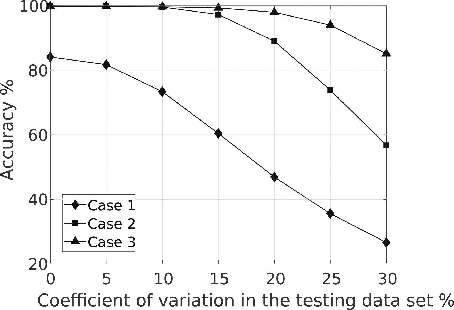
Multi-sourced uncertainties
To examine the effect of multi-sourced uncertainties on the proposed method, Cases 4, 5, and 6 have been created and tested using the testing dataset described in Table 1. Case 4 has uncertainty in the Damping Ratio and Modulus of Elasticity, Case 5 has uncertainty in the mass density, modulus of elasticity, and Case 6 has uncertainty in the mass density, damping ratio, and modulus of elasticity. All these cases has tested using T1 from Table 2.
Case 3 from the previous study (single-sourced uncertainties) is compared to Cases 4-6 as seen in Figure 8. As expected, Case 6 has shown the best result among the other cases, but the overall performance of all cases is similar to each other. Adding multi-sourced uncertainty in the training dataset slightly increases the CNN model performance compared to Case 3. This indicates that using single-sourced uncertainty in the modulus of elasticity (i.e., Case 3) is essential and sufficient, simplifying the training dataset preparation without sacrificing the overall performance of the method. As long as there is 20% uncertainty in the elastic modulus in the training data, the CNN model was able to detect the impact force location with over 97% accuracy for 20% uncertainty in the testing data and over 94% accuracy with 25% uncertainty in the testing data. Once the uncertainty level in the testing data exceeds 30%, the impact force location identification accuracy drops below 90% as shown in Figure 8. Impact load location identification accuracy for Case 3-6 with different CV of the testing data.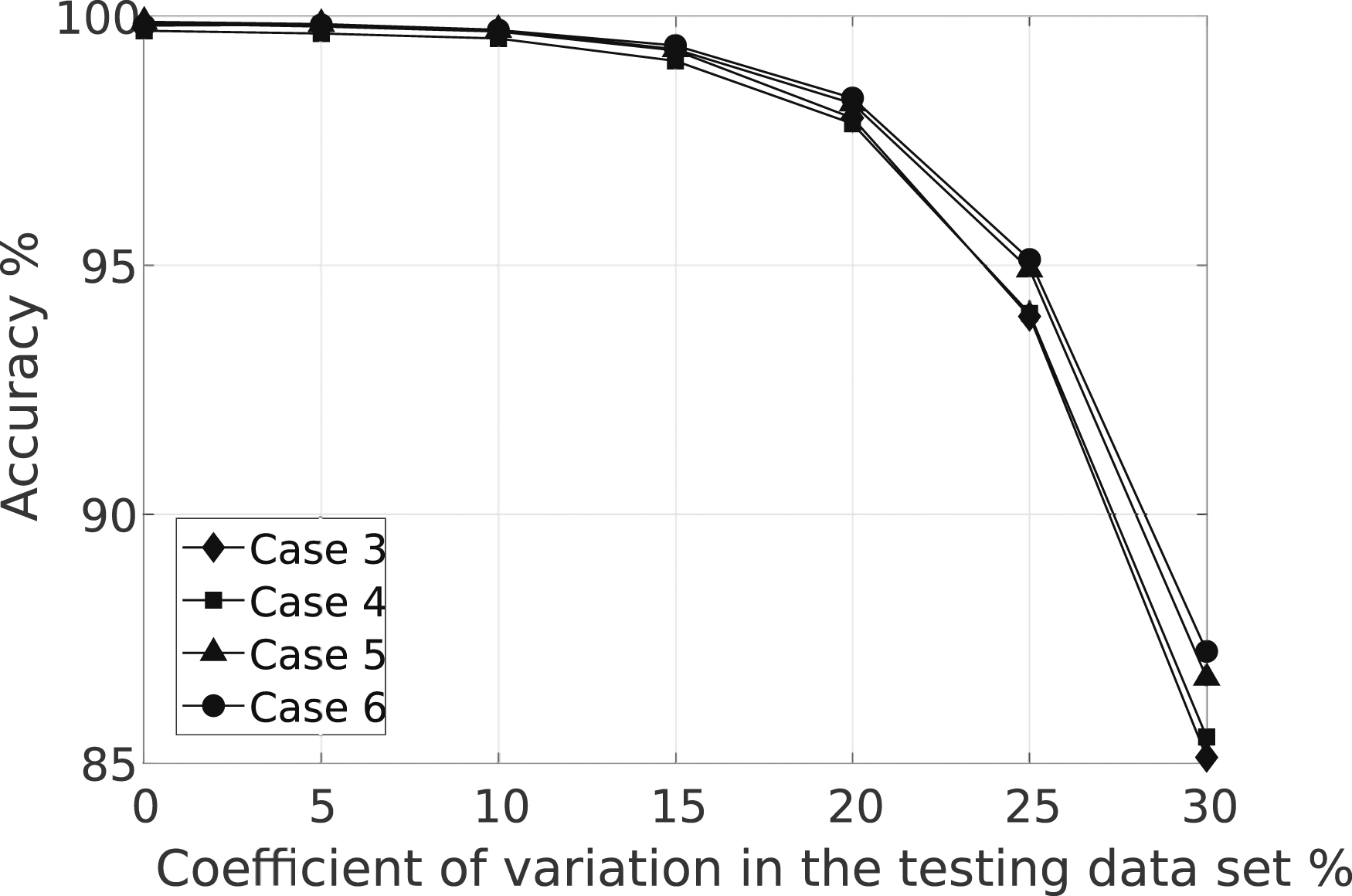
Effect of different level uncertainties
An additional case (i.e., Case 7) was investigated to examine the effect of different CV levels between the training and testing datasets, as described in Table 1. This study extends the analysis to CV levels up to 60% and tested using T2 of Table 2. The results of this study are shown in Figure 9. Impact load location identification accuracy for Case 7 with different CV of the training and testing data.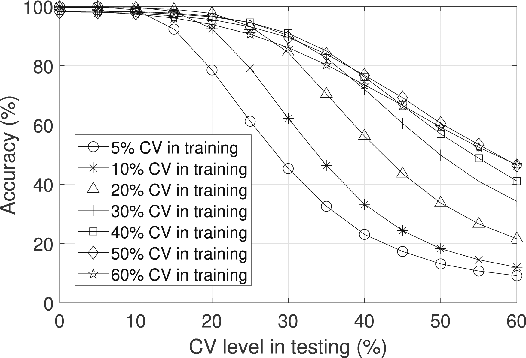
As long as the CV levels in the training data are equal to or higher than those in the testing data, the CNN model was able to locate the impact force with over 90% accuracy. If the uncertainty level of the testing dataset was higher than the training dataset, the model can identify the location of the load in some cases. For example, if the CNN model was trained using a CV level of 5%, the model was able to locate the force with a CV level of 15% in the testing dataset with an accuracy of over 90%. If the CV level is 10% in the training dataset, the model can locate the load (90% accuracy) up to 20%.
Models trained with CV levels of 30% or higher demonstrated stronger generalization. However, beyond 40%, the accuracy gains were minimal, with models trained using 50% and 60% CV showing almost identical performance. This indicates that increasing the CV level in training beyond a certain point does not lead to substantial accuracy improvements.
Task 2 - Impact load magnitude identification
The magnitude of the impact load for the training dataset was set between 5 and 80 N, stepped by 5 N. For each magnitude value, ϕ was set between 0 and 180°, and θ between 0 and 360°, both stepped by 10°. This configuration was applied to each of the 44 possible impact load locations, resulting in 10,096 data points for training at each location. Additionally, a testing dataset of 10,000 samples was generated with uniformly random magnitudes and directions in each location. The magnitudes were set between 5 N and 80 N, ϕ was set between 0 and 180°, and θ between 0 and 360°, with a given sensor location at node 13. In this task, Case 8 of Table 1 was used for training and T3 of Table 2 was used for testing.
Figure 10(a) presents a box chart illustrating the percentage error in magnitude estimation across various load locations. The plot reveals a mean absolute percentage error of about 3.68%, with the upper quartile ranging from 3% to 8%. Notably, the performance of magnitude estimation improves when the impact load is applied in proximity to the sensor location (i.e., node 13). Turning to Figure 10(b), another box chart depicts the percentage error associated with changes in impact load magnitude. In this figure, the method successfully estimates the impact load magnitude regardless of the magnitude levels, achieving an upper quartile error of 5% and a mean error of 3.68%. This test demonstrates the method’s proficiency in identifying the magnitude of the impact load, even in the presence of uncertainty. Box chart of the distribution of average load magnitude estimation error with change in force: (a) Location, (b) magnitude.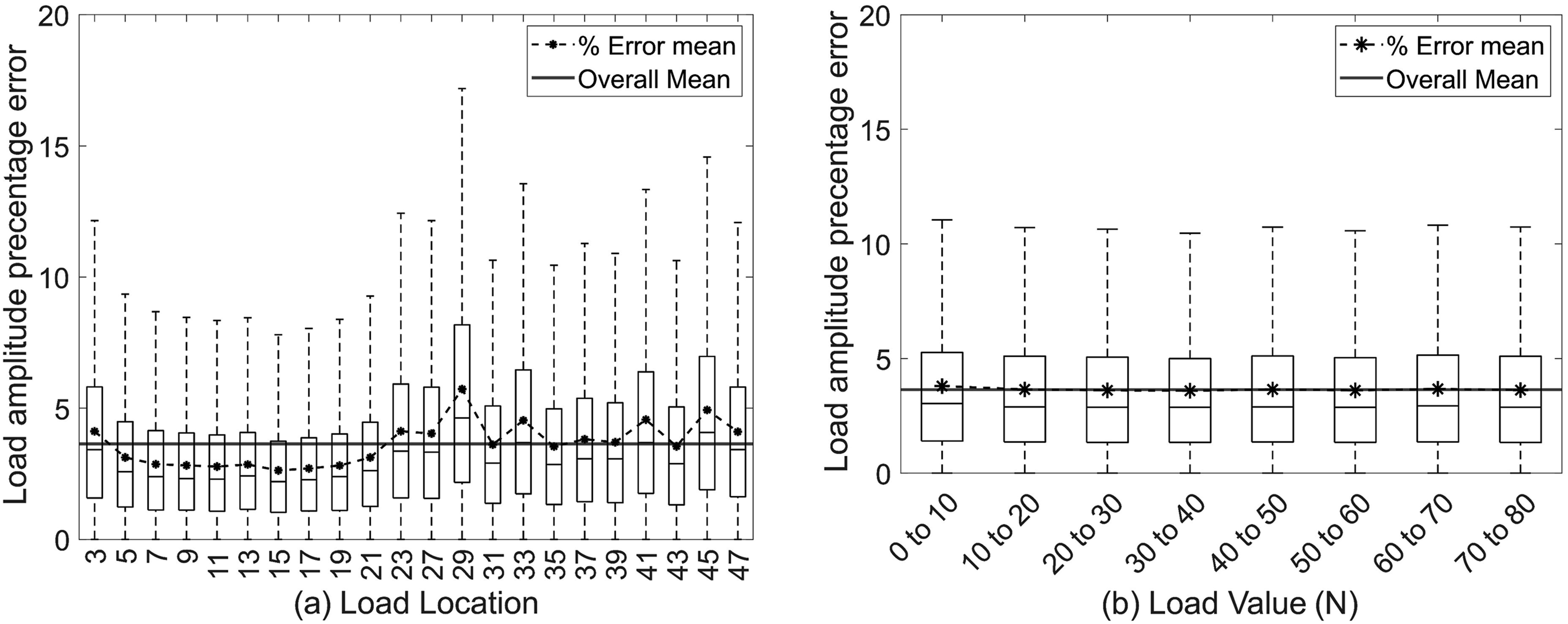
To examine the effect of various CV levels on the method’s performance, Case 7 from Table 1 (up to a CV level of 30%) and T1 from Table 2 were used. As shown in Figure 11, the model was able to identify the magnitude of the impact load with less than 5% error for the cases having up to 10% of CV in the testing dataset. In general, as the uncertainty level (CV) in the testing data increases, the magnitude identification error also increases to close to 10% for the 30% CV cases in the testing data. Additionally, a CV level of 30% in the training dataset yields lower performance compared to the other CV levels in the training dataset. In general, using a CV level of 20% in the training dataset demonstrates better performance compared to other CV levels in this test. Different value of coefficient of variation (CV) of the training data set and testing data set of Task 2.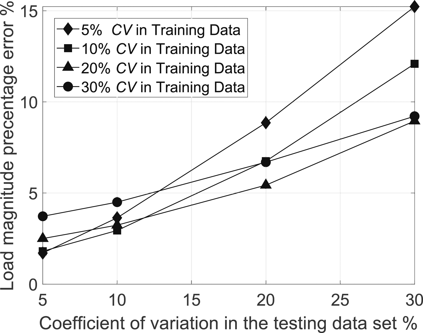
Task 3 - Impact load direction identification
To identify the direction of the impact load, another CNN model was developed. The training and testing datasets described in the previous section (Task 2) were used. After the CNN model was trained and tested, the method successfully estimated α, β, and γ with a mean absolute error of 1.95°, as shown in Figure 12. Additionally, Figure 12(a) presents a box chart illustrating the distribution of the estimated absolute errors for α, β, and γ. From the figure, the lower and upper quartiles are approximately 0.72 and 2.8°, respectively. (a) Box chart of the distribution of average angle estimation error of α, β, and γ. (b) Box chart of the distribution of average Direction angle estimation error with change in force: (a) location, (c) magnitude.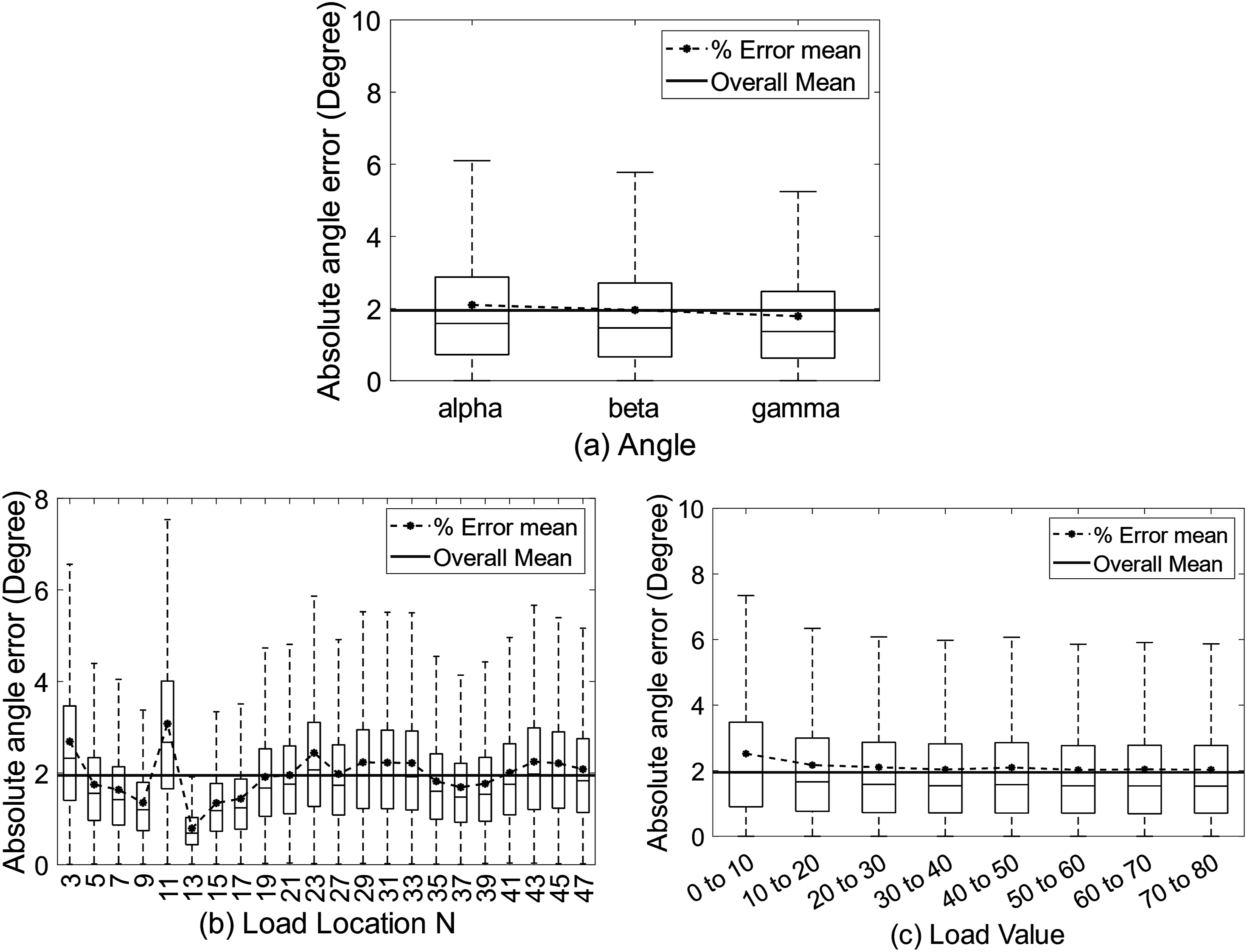
The effects of changes in the impact load location and magnitude on the direction estimation error are depicted in Figure 12(b) and (c). As shown in Figure 12(b), as the load is applied closer to the sensor location (i.e., node 13), the absolute error decreases. Figure 12(c) indicates that when the impact load magnitude is relatively low, the direction estimation error is slightly higher than in other cases. However, overall, the impact load magnitude has a minimal effect on the method’s performance in estimating the direction of the load, as seen in Figure 12(c). The test results demonstrate the method’s capability to estimate the direction of the load accurately even in the presence of uncertainty.
To evaluate the performance of the method across different levels of the coefficient of variation (CV), we used the training and testing datasets described in the previous section (Task 2). The results are shown in Figure 13. The method was able to accurately identify the direction of the impact load, achieving a mean absolute error of less than 6.5° for CV levels up to 30% in the testing dataset. This accuracy was maintained as long as the model was trained with sufficiently high CV levels (e.g., 20% and 30%). For testing datasets with lower CV levels (up to 10%), all training datasets resulted in a mean absolute error of less than 5°. Different value of coefficient of variation (CV) of the training data set and testing data set of Task 3.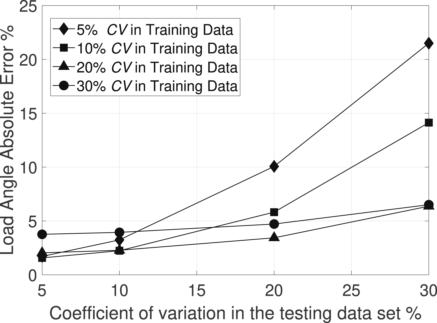
Effect of different sensor locations
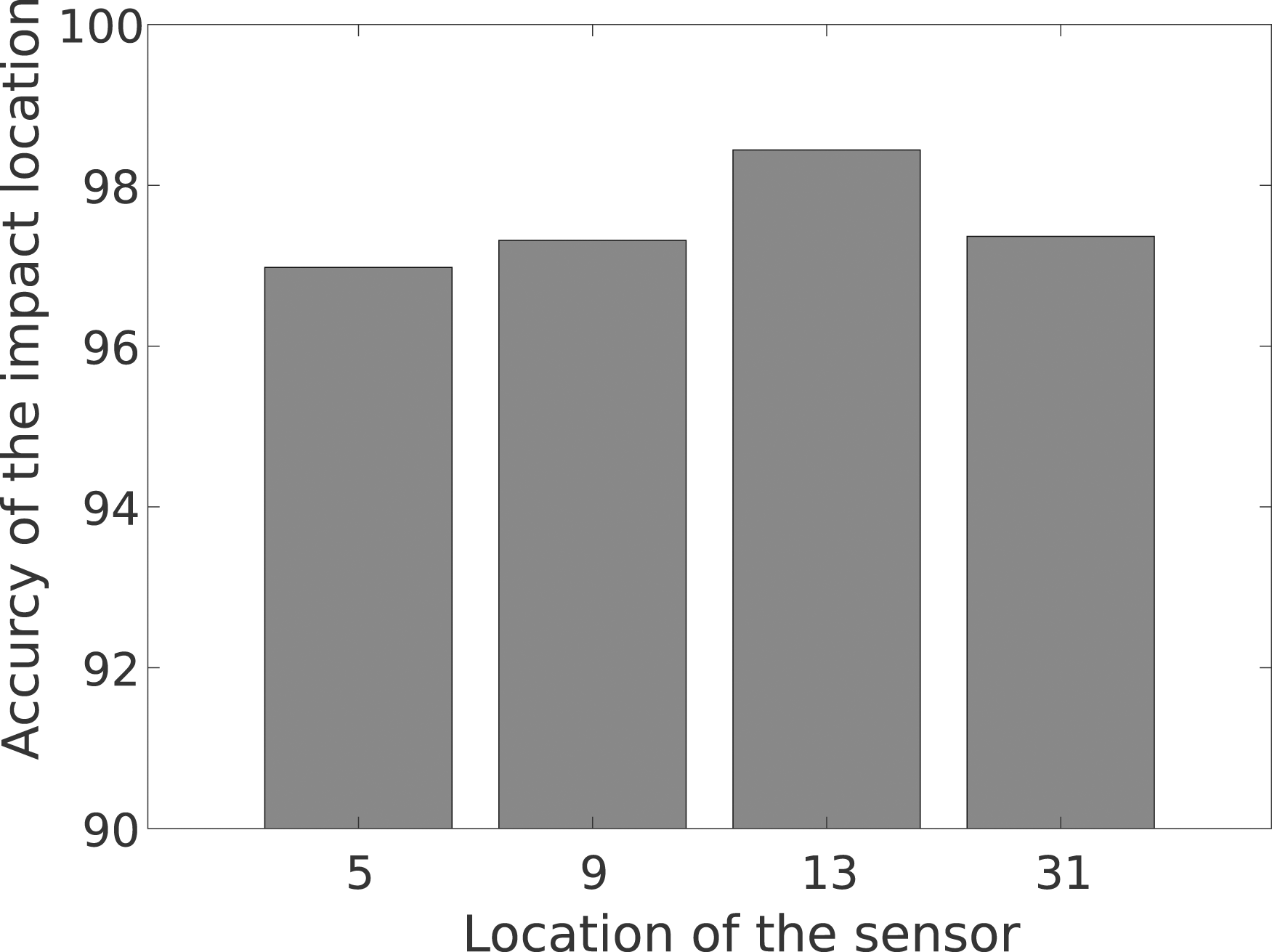
In practice, placing a sensor in a specific location is not always available or may be difficult to install due to limited accessibility. In general, a different measurement location can provide different performance in analyzing the structure (Saleem and Jo, 2021). To check the effect of different measurement locations on the performance of the method, Case 8 and T2 was used to identify the impact load location. As illustrated in Figure 14, four example cases of different sensor locations were considered, and the results are presented in Figure 15. As seen in the figure, regardless of the sensor location, more than 95% accuracy of location identification was obtained, implying that the sensor location has little effect on the performance of the method. Different location cases. Sensor location effect on location identification accuracy.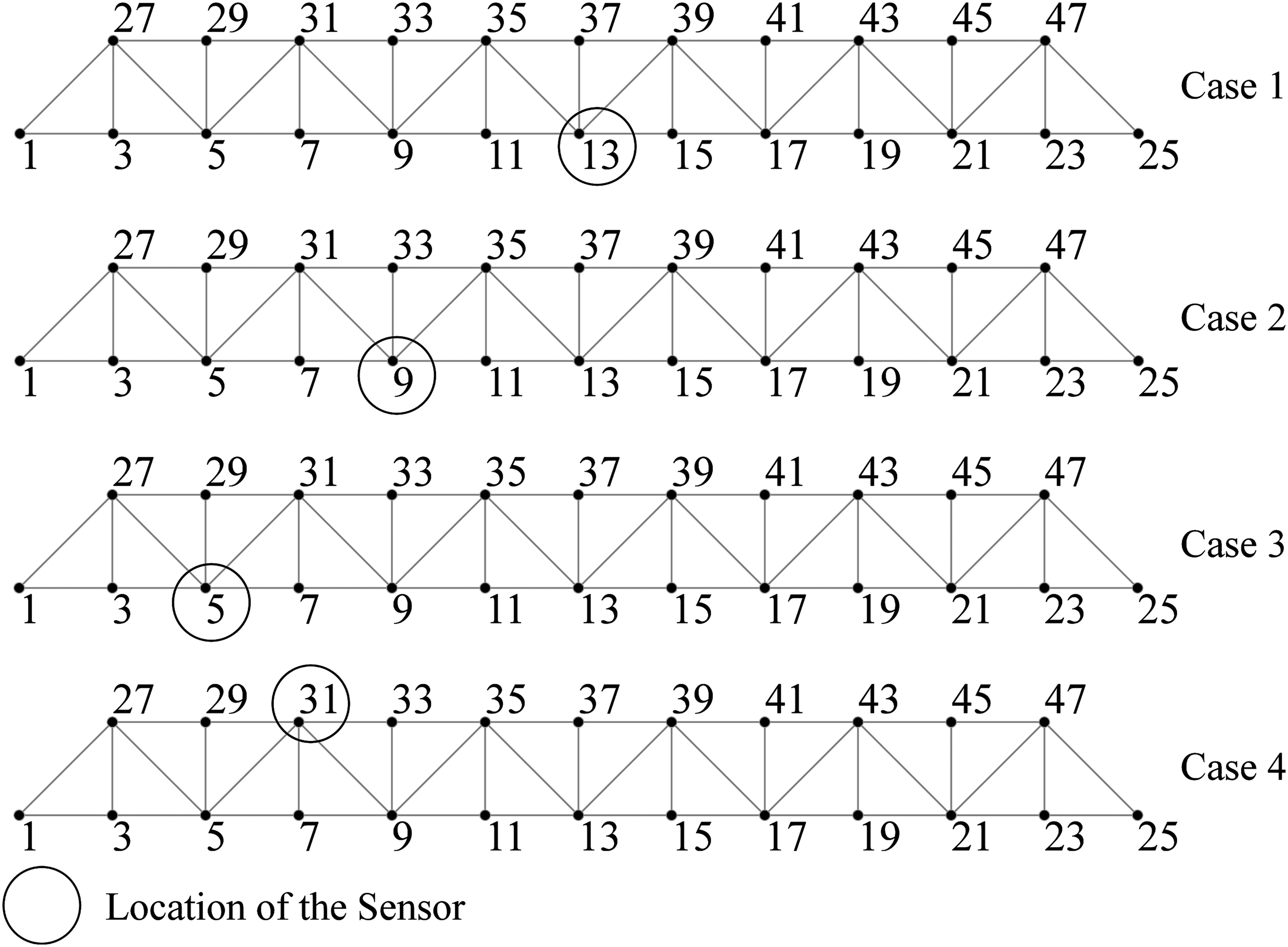
Effect of different architectures and hyperparameters
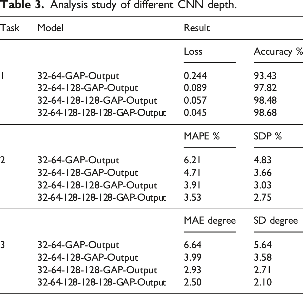
Analysis study of different CNN depth.
Effect of boundary condition uncertainty
To assess the impact of boundary condition (BC) uncertainty on the performance of the proposed method, the truss structure model was modified. In this setup, the boundary nodes (1, 2, 25, and 26) are constrained in the y and z directions but remain free in the x direction. An adjustable stiffness k
x
in the x direction was introduced to simulate varying levels of BC uncertainty, as shown in Figure 16. When k
x
= 0, the truss supports are free in the x direction, and when k
x
→ ∞, they approximate pinned supports. Truss structure with adjustable boundary condition stiffness in the x-direction.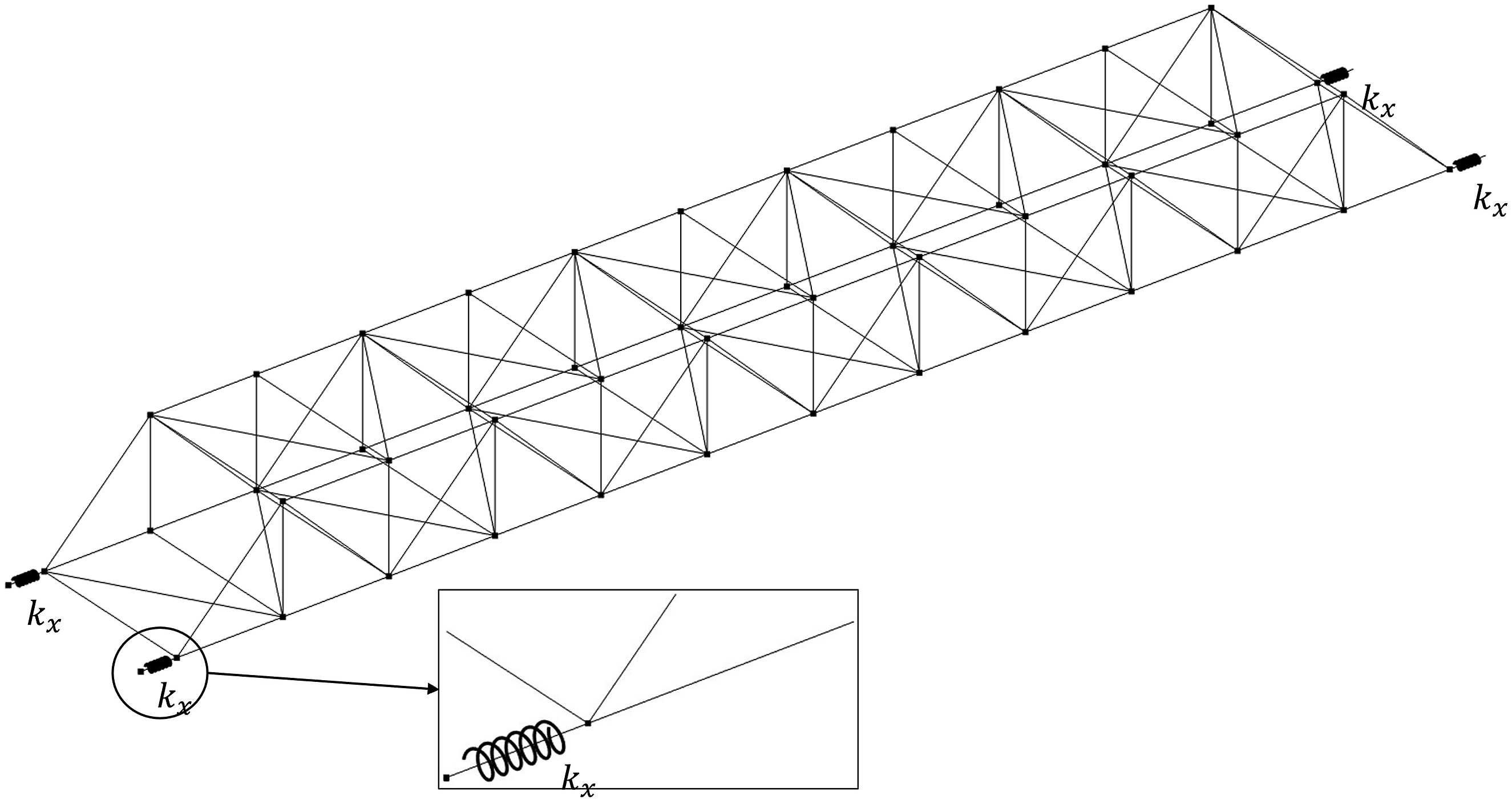
To determine a suitable mean value for k x , impact loads were applied at node 38 in both the original truss (Figure 5) and the modified truss (Figure 16) with identical force characteristics: 20 N magnitude, applied at a 45° angle in both horizontal and vertical planes. The acceleration responses for different k x values were recorded for the modified truss.
Figure 17 presents the difference in acceleration responses between the two trusses, evaluated using mean absolute error (MAE) and normalized cross-correlation (NCC), defined in Appendix B. As k
x
increases, MAE decreases, and cross-correlation improves, indicating closer alignment between the response behaviors of the two truss setups. A mean value of k
x
was chosen as 3.1623 × 10¹⁰ N/m based on these trends to represent typical BC uncertainty for subsequent analyses. Effect of boundary condition stiffness k
x
on acceleration response of both truss.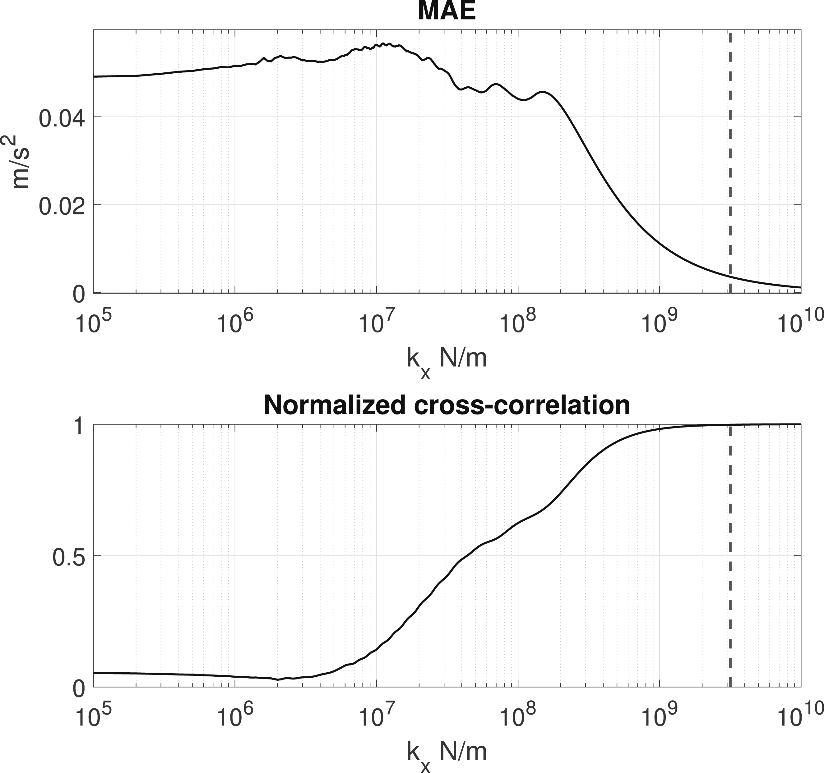
Tasks 1, 2, and 3 were re-evaluated to incorporate BC uncertainty and were compared to cases without this additional uncertainty.
Task 1 - Impact load location identification
In this task, two training and two testing datasets were prepared to examine the effect of BC uncertainty on the performance of the proposed method. The first training dataset considered only uncertainty in the modulus of elasticity (Case 9), while the second included both modulus of elasticity and BC uncertainties (Case 10), as summarized in Table 1. Testing was performed using datasets T2 (no BC uncertainty) and T4 (with BC uncertainty), detailed in Table 2.
Two CNN models were trained, one with Case 9 and another with Case 10. Initial testing on the T2 dataset revealed similar performances for both models, as shown in Figure 18(a). Further testing with the T4 dataset also showed consistent results (Figure 18(b)), demonstrating that incorporating BC uncertainty in the training phase did not significantly affect model performance. Thus, including only modulus of elasticity uncertainty in the training data proved effective. Comparison of CNN Model Performance with and without Boundary Condition Uncertainty: (a) Tested on Dataset T2 (no BC uncertainty) and (b) Tested on Dataset T4 (with BC uncertainty).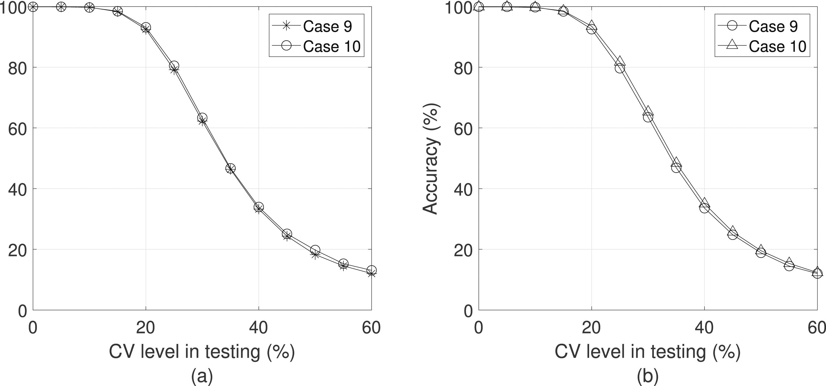
Tasks 2 and 3 - Impact load magnitude and direction identification
To examine BC uncertainty’s effect on impact load magnitude and direction identification, two training datasets were prepared. Case 8 included only modulus of elasticity uncertainty, while Case 11 incorporated both modulus of elasticity and BC uncertainties, as outlined in Table 1. Testing datasets T3 and T5 were used, with T5 including BC uncertainty.
CNN models trained with Cases 8 and 11 were first tested on T3, yielding a mean absolute percentage error (MAPE) of 3.68% for Case 8 and 4.0% for Case 11 in load magnitude identification. For direction identification, the mean absolute error (MAE) was 1.95° in both cases. Subsequent testing with T11 confirmed similar results: MAPE remained at 4.0% for magnitude, with direction MAE at 2°. This reinforces that modulus of elasticity uncertainty alone in the training data sufficiently captures the model’s variability requirements, with BC uncertainty adding no notable performance benefit.
Summary and discussion
From this numerical case study, the method was able to identify the location, magnitude, and attacking direction of the impact load using just a single tri-axial accelerometer. In addition, the Physics-based simulator was used to generate the training data, and the performance was evaluated with various cases as presented above. From these tests, the following conclusions were drawn: • If the CV levels in the training data are sufficient, the method can effectively identify the impact load for uncertain systems. • The method can identify the impact load with a high uncertainty using a high level of CV in the training dataset. This indicates that the method can be trained using high CV if needed, without sacrificing the overall accuracy.
Laboratory case study
The proposed methodology has been validated through a laboratory setup. As previously mentioned, bridges with stringers/multi-beams or girders are commonly used (Farhey, 2018). Furthermore, vehicle collisions (i.e., impact loads) represent one of the primary causes of bridge failures (Zhang et al., 2022). Consequently, a beam fixed at both ends was selected for the study. The experimental settings are shown in Figure 19, and the parameters of the beam are outlined in Table 4. Since the impact load was only applied in one direction in the beam, only the impact load location and magnitude were identified using a single accelerometer (PCB Piezotronics 352C33). To verify the accuracy of the estimated impact load, an impact hammer (DYTRAN 5800 Series) was used to provide the reference data. The accelerometer was positioned at 0.4572 m (18 inches) from the right support, as illustrated in Figure 20. The impact load location varied every 0.1524 m (6 inches) with different magnitudes, resulting in seven potential impact locations. In this experiment, a physics-based simulator of the beam was used to generate training data numerically, as described earlier in the section on physics-based simulation, and subsequently tested the performance of the method with laboratory measurements. The stiffness matrix was constructed using the stiffness method (Hibbeler and Tan, 2006; Mario and Young, 2019) and the mass matrix was constructed using Consistent Mass method (Mario and Young, 2019). In both method, 54 beam segment have been used. The damping matrix was constructed using 0.02 of damping ratio. Experimental setup. Beam parameters. Geometry of fixed-fixed beam and distribution of impact load location.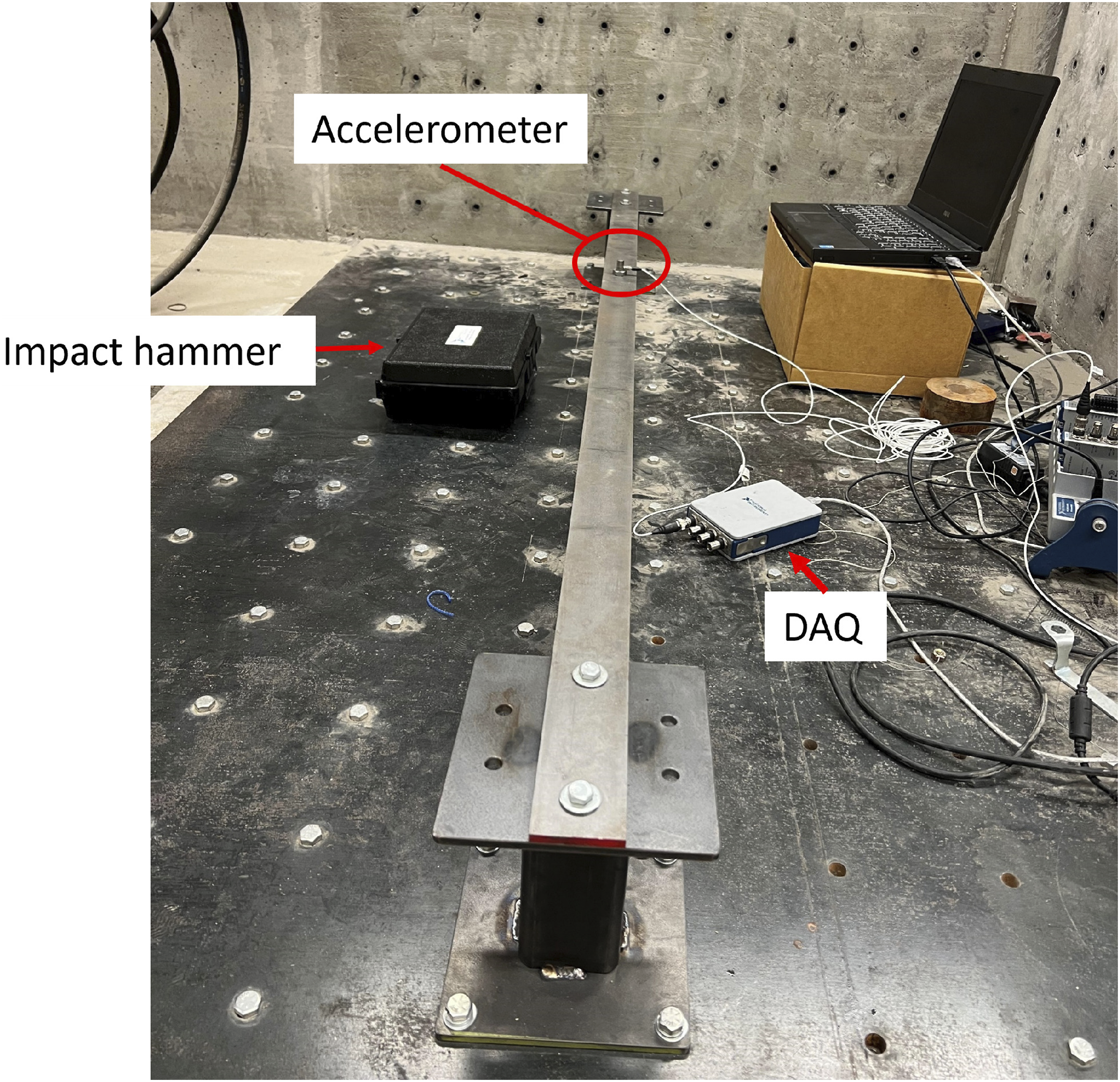
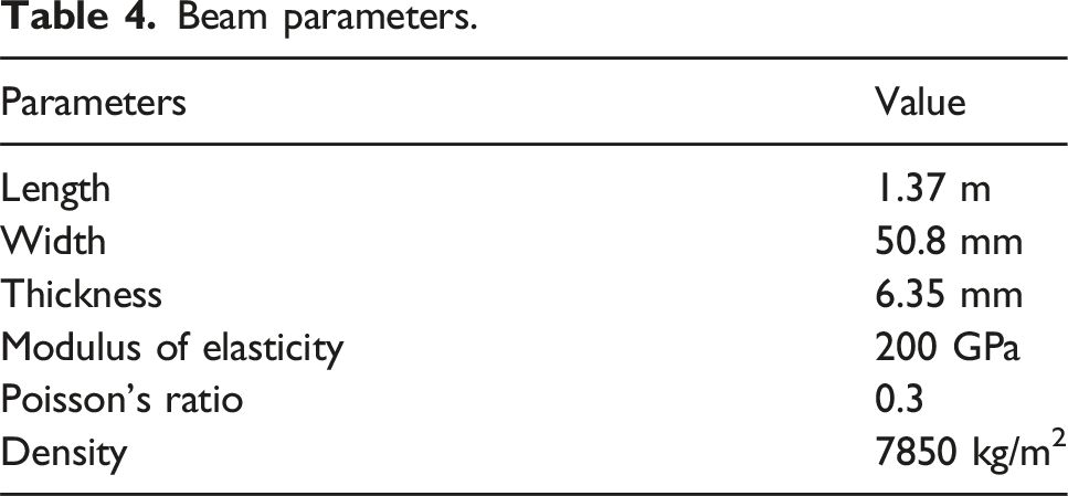
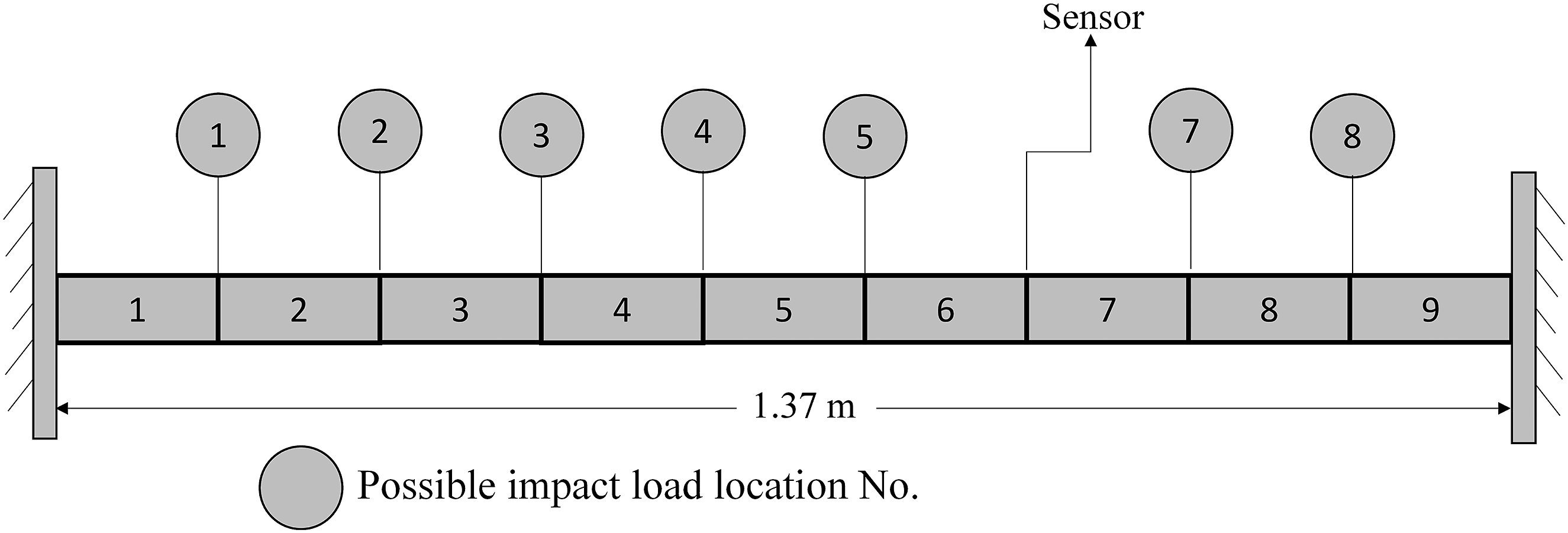
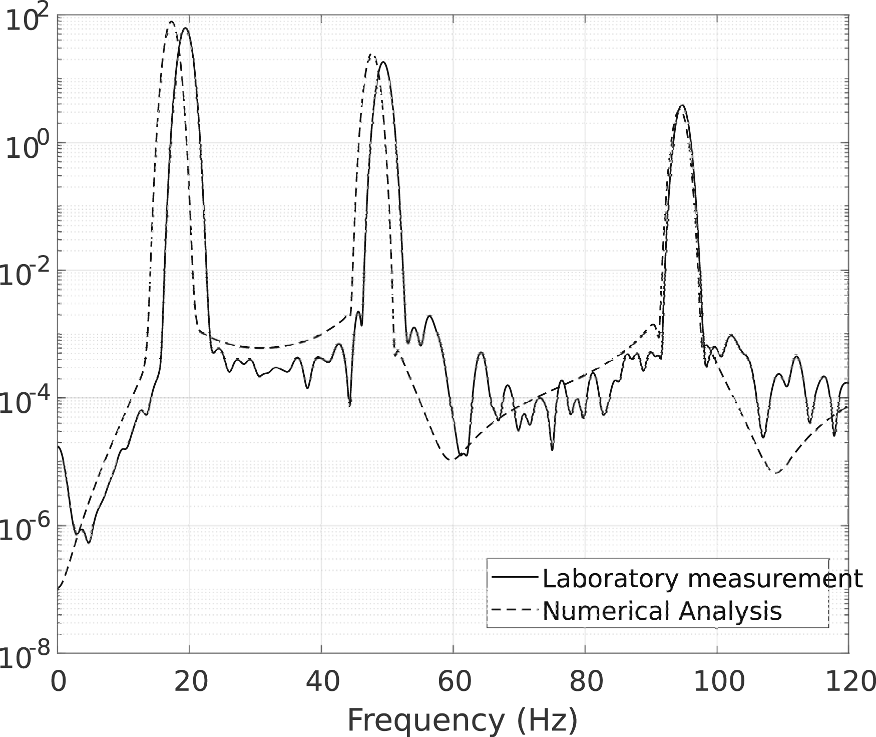
Figure 21 shows that both simulated data and lab measurements of example impact loads and acceleration responses match well in the time domain. Figure 22 shows the frequency‐domain comparison of the simulated and measured acceleration response. The model parameters were considered in the physics-based simulator for this test. Time history of the impact load excitation at location No. 4 and acceleration response of the accelerometer for Numerical Simulation and Laboratory measurement. The power spectral density function of the acceleration response of the accelerometer due to the impact load at location No. 4.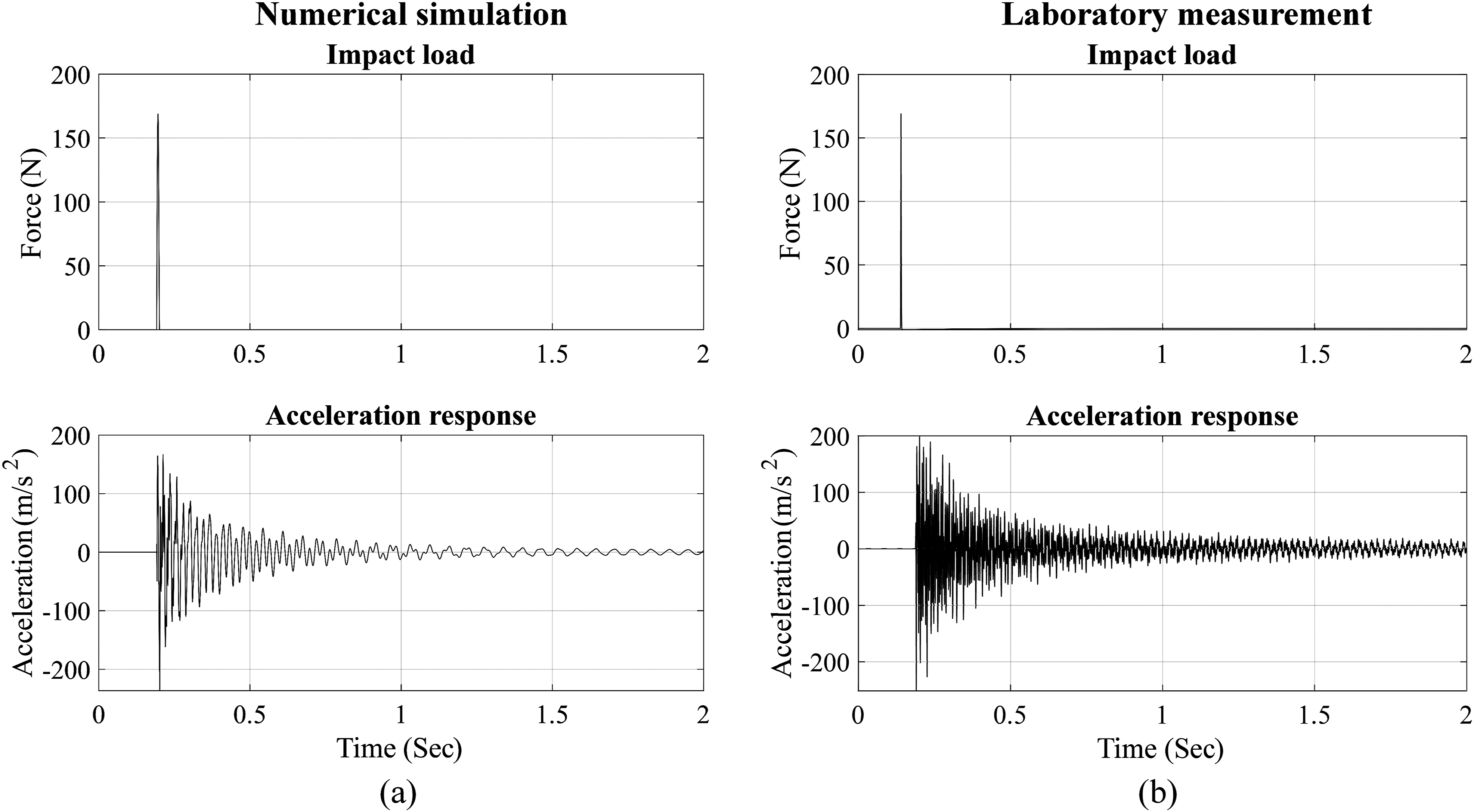
Experimental results
Task 1 - Impact load location identification
For the location classification training, a total of 23,100 samples of data were used, which were generated using the physics-based simulator at 2000 Hz sampling frequency and a time span of 0.15 seconds. As a result, the input size for the CNN model is (1,300). The testing dataset consisted of 147 samples collected from the laboratory tests. Each sample in both the training and testing sets underwent filtering using a low-pass filter with a cutoff frequency of 100 Hz. The training data were generated with varying levels of uncertainty (i.e., 0%, 5%, 10%, 15%, 20%, 25%, 30%, and 40%) in the modulus of elasticity, as it demonstrated strong performance in the previous numerical case study.
Figure 23 shows the accuracy of location identification as the uncertainty level considered in the training data increases. Initially, without including the uncertainty during the training, the CNN model struggled to find the impact load’s location. This difficulty was particularly evident in the discrepancies observed between the numerical analysis and laboratory measurements, as shown in Figure 22, which was a predictable and intentional outcome. However, as the uncertainty level increased, the accuracy of load localization gradually improved. Notably, the model achieved 98% accuracy when the uncertainty level reached 10%. Impact load location classification accuracy with different CV in the modulus of elasticity.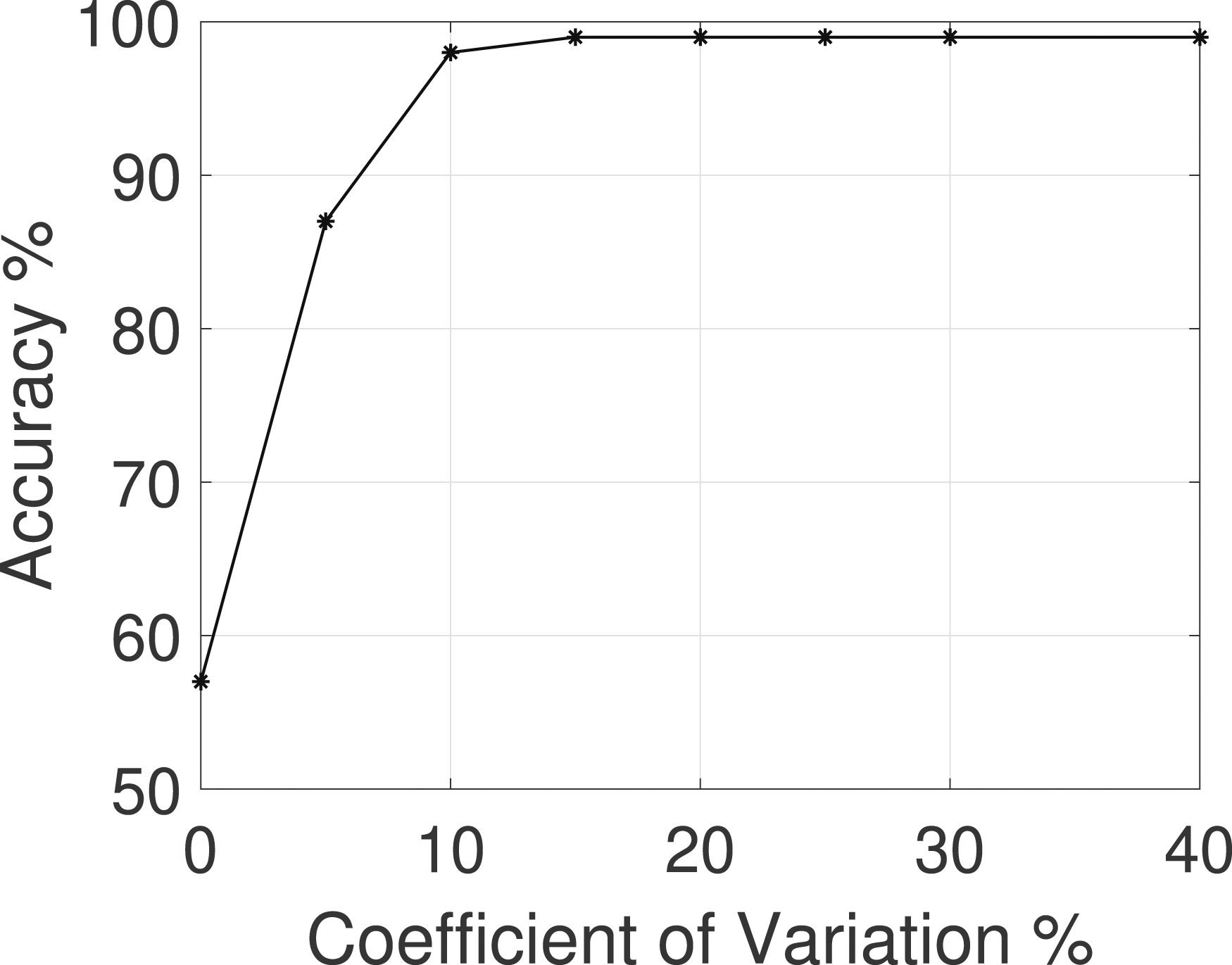
Task 2 - Impact load magnitude identification
To examine the CNN method for the impact load magnitude estimation, a separate CNN model was created for each possible location and trained with 15,150 samples. Following the model training, it was tested and evaluated using the laboratory measurements. Figure 24 illustrates the percentage absolute error of the estimated impact load magnitude. As depicted, the mean absolute percentage error across all locations amounts to 2.2%, with a maximum error of 6%. Notably, the error decreases when the load is applied closer to the sensor location (i.e. between the node 5 and 7). These test results also demonstrate the CNN method trained using a simulator data can accurately estimate the magnitude of the impact load in the laboratory tests. Estimated impact load magnitude percentage absolute error of every location.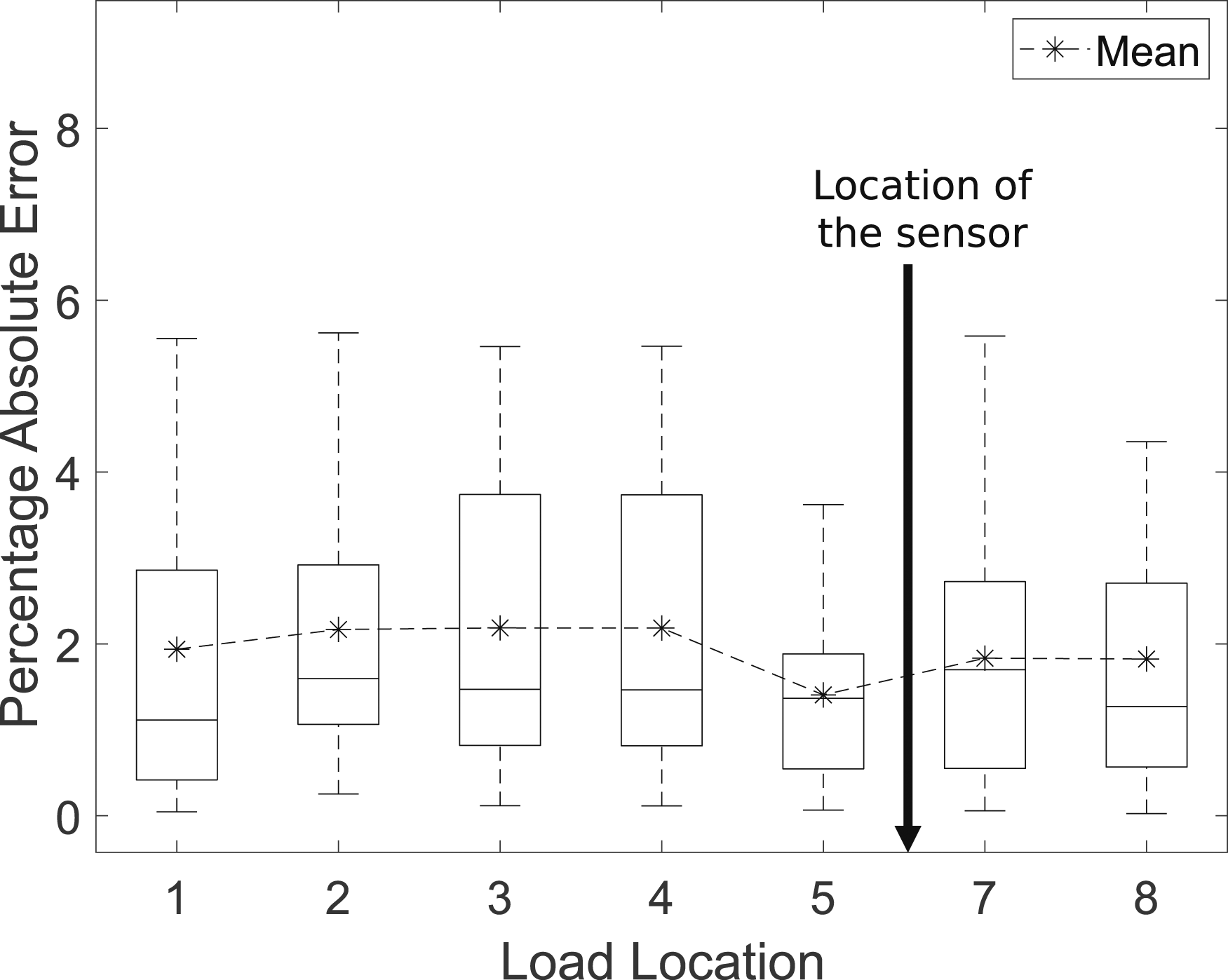
Conclusion
This paper presents a novel CNN-based method for impact load identification. The proposed method can identify the location, direction, and magnitude of the impact load using a single measurement point, even in the presence of parameter uncertainties. Additionally, this is the first method that used a Physics-Based simulator to generate the training data for the dynamic load identification. The effectiveness of this method was validated through both numerical and experimental case studies, considering possible uncertainties in the model parameters. Particularly, the Physics-based simulator proved to be effective in providing the necessary training data for the CNN model and the ability of training the model with high uncertainty. This showed the potential of real-world applications as shown in the laboratory tests.
Considering the modulus of elasticity, mass density, and damping ratio as uncertain parameters in physical-based simulations showed great performance. And the way of employing such uncertainties in this method highlights its flexibility in addressing different sources of uncertainties and its potential for application to more complex structures in future studies. In cases where only using these parameters is insufficient, more detailed modeling will be necessary to ensure correct prediction of structural behavior.
Footnotes
Appendix A
The custom normalization layer is designed to reduce the magnitude effect of the force in the acceleration response. Consider two individual acceleration responses
where c is a scale factor. Considering the equations of motion (Equation 1):
From the equations above, we can write:
By comparing the left and right sides of the equation, we get:
Therefore, we can relate
We see that the difference between
Let the function MAX(XIn) be:
where
If
The term c/|c| is either 1 or −1 depending on the sign of c. Since the direction of
For this example, Equation 29 is only true if the location and direction of
As a result, the custom normalization layer can reduce the magnitude effect of the impact load on the acceleration response and increase the performance of the CNN model in identifying the location and the direction of the impact load.
Appendix B
To test the performance of the proposed method, different indices are used and defined below:
Task 1 - Impact load location identification
Categorical cross-entropy loss function (Loss)
Where
And
Task 2 - Impact load magnitude identification
The Mean absolute percentage error (MAPE)
To find the standard deviation of percentage errors (SDP), the percentage error (PE) of each sample should be found first
Then
Task 3 - Impact load direction identification
The Mean Absolute Error (MAE)
To find the standard deviation (SD)