Seismic response of a large,isolated aqueduct considering fluid–structure and soil

Abstract

To investigate the seismic responses of a large, isolated aqueduct, a three-dimensional fluid–structure–soil interaction model was established using the arbitrary Lagrangian–Eulerian (ALE) method and the dynamic Winkler foundation model. Frictional pendulum bearings were modelled using a simplified model consisting of a simple pendulum and a non-linear spring. In addition, the uniform and non-uniform seismic excitation models without considering pile–soil dynamic interactions were established to analyse the effects of pile–soil dynamic interactions and the seismic input method on the seismic response analysis of the large-scale aqueduct. The feasibility of the numerical approaches used in this study was verified by examples. The isolation effect and deformation of the frictional pendulum bearings, the stress distribution of the piers, and water sloshing were then analysed. The simulation results showed that the frictional pendulum bearings provided a good seismic isolation effect and that it is necessary to consider the dynamic interactions of pile–soil–aqueduct structures in the seismic analysis of large-scale aqueducts.

Keywords

aqueduct ALE fluid–structure interaction model friction pendulum bearing pile–soil dynamic interaction seismic response

Introduction

To change the uneven distribution of water resources in China and promote the coordinated development of the economy, resources, and environment, the South-to-North Water Diversion Project was proposed, in which aqueducts play a very important role as water transport structures across valleys and rivers. The large-scale aqueducts, as class-I structures, have high seismic fortification requirements (GB51247-2018, 2018). Thus, it is necessary to study their seismic responses in detail.

However, since the whole aqueduct structure is a complex system consisting of water, an aqueduct tank, bearings, piers, piles, and soil, its seismic response analysis involves complex fluid–structure–soil interaction problems. The first problem is the fluid–structure interaction problem between the water and the aqueduct tank. The water will slosh with the seismic motion of the tank, and in turn the water sloshing will change the natural vibration characteristics of the aqueduct structure and affect its dynamic responses. The main solutions include Westergaard’s additional mass method (Westergarrd, 1933), Housner’s method (Housner, 1957), the boundary element method (Nakayama and Washizu, 1981), and the arbitrary Lagrangian–Eulerian (ALE) finite element method (Hirt et al., 1974). However, Westergaard’s additional mass method ignores the effects of water sloshing on the dynamic responses of the structure, Housner’s method cannot reflect the internal force distribution of the aqueduct tank and has limited application, and the boundary element method ignores the effects of the aqueduct on the water. Previous studies (Kim et al., 2002; Zhang et al., 2013a, 2013b) have shown that the ALE method combines the advantages of the pure Lagrangian method and the pure Eulerian method. It is a better choice for solving nonlinear fluid–solid coupling problems, and it can fully consider the coupling effects of both water and the structure.

The other critical problem is the pile–soil dynamic interaction problem. The pile group foundation has been widely adopted in large-scale aqueducts to improve the subgrade bearing capacity and control the settlement of the aqueducts. Previous studies (Maheshwari et al., 2004; Soneji and Jangid, 2008; Song et al., 2023) have shown that the pile–soil dynamic interactions have significant effects on the seismic responses of the superstructure. The accurate solution is to establish a complete finite element model of the pile and soil, which can consider not only the seismic responses of the soil but also the relative motions between the pile and soil (Li et al., 2021; Luo et al., 2016). However, the computational efficiency is too low for large-scale models, and the Winkler foundation model may be a better choice. In the Winkler foundation model, the pile and soil models are simplified using beam elements and linear spring elements, respectively. Novak (1974), Novak et al. (1978), Gazetas and Makris (1991) and Makris and Gazetas (1992) improved the Winkler foundation model and applied it to the seismic response analysis of soil–pile–structure interaction systems. Some studies (Chen et al., 2012; Kildashti et al., 2016) also showed that the dynamic Winkler foundation model could promote computational efficiency and is suitable for the seismic response analysis of large-scale models.

Based on these methods, some studies have been conducted on the seismic responses of aqueducts (Li et al., 2003; Valeti et al., 2016; Wu et al., 2023; Xiao et al., 2021; Xu et al., 2021; Zhang et al., 2013a; Zhang et al., 2022a; Zhang et al., 2022b). Zhang et al. (2013b) investigated the dynamic responses of an aqueduct–water coupling system under earthquake and wind loads and found that the isolated technique improved earthquake resistance of the aqueduct structure but reduced the wind resistance performance of the aqueduct bridge. Zhang et al. (2022a) carried out seismic response analysis and reliability research of an aqueduct structure and found that the influence of the randomness of seismic excitation on the seismic response and seismic reliability of the aqueduct was significantly higher than the influence of the randomness of the concrete parameters. Zhang et al. (2022b) investigated the fragility of an aqueduct system under the excitation of near-fault pulse-type (NFP) and far-field (FF) ground motions and found that the fragility probability of a high-span aqueduct system under NFP ground motions was significantly greater than that under FF ground motions. However, most studies only focused on the superstructure or did not consider water as a fluid, and the aqueduct in the simulation was only a segment rather than a large-scale structure. There have been limited studies on the seismic response analysis of the large-scale aqueduct structure considering the fluid–structure–soil interactions simultaneously. In addition, the frictional pendulum bearing has been widely used in building and bridge structures as a seismic isolation device, and its isolation effect in aqueduct structure was also worth investigating.

The fluid–structure–soil interactions play a critical role in the seismic responses of aqueducts, and neglecting any of these will lead to an incorrect estimation of the seismic response. Therefore, based on the large-scale aqueduct of Pi River in the Yangtze River–Huai River Water Diversion Project, a three-dimensional fluid–structure–soil interaction model was established using three-dimensional finite element software ABAQUS (Dassault Systemes Simulia Corp., 2014) to investigate the seismic responses of the whole large-scale aqueduct in this study. The main trusses, rebar cages of piers, and frictional pendulum bearings were considered in the simulations, and viscoelastic artificial boundaries were placed at the two ends of the waterbody to simulate the free boundary of water motion. Furthermore, the uniform and non-uniform seismic excitation models without considering pile–soil dynamic interactions were also established to analyse the critical roles of pile–soil dynamic interactions and the seismic input method in the seismic response analysis of the large-scale aqueduct. It is hoped that the findings of this study could shed some light on the seismic fortification of large-scale aqueducts.

Description of numerical approach

In this section, the numerical approaches used in this study are introduced, and their feasibilities are verified through examples.

Arbitrary Lagrangian–Eulerian (ALE) fluid–structure interaction model

The ALE adaptive meshing technique is a hybrid method that combines the features of pure Lagrangian analysis and pure Eulerian analysis (Hirt et al., 1974). ALE adaptive meshing consists of two main processes: creating a new mesh and remapping solution variables from the old mesh to the new mesh. It can maintain a high-quality mesh without changing the topology (elements and connectivity) of the mesh by allowing the mesh to move independently of the material. Some previous studies and an ABAQUS example of water sloshing in a baffled tank have shown that the ALE method was applicable to solve fluid–structure interaction problems in the case of large-amplitude water sloshing (Zhang et al., 2013b, Dassault Systemes Simulia Corp., 2014).

However, the tank was rigid in the ABAQUS example, but the solid elements were required in aqueduct model. Therefore, to further validate the applicability of the ALE method in fluid–structure interaction problems when the structures were modelled by solid elements, the ABAQUS example was re-simulated using a solid tank in this study. The model geometry is shown in Figure 1(a). The tank was filled with 101.6 mm of water. The tank measured 508 × 152.4 × 152.4 mm, and the baffle measured 3.048 × 152.4 × 121.92 mm. The thickness of the solid tank was set to 30 mm. The model parameters of the solid tank, baffle and water can be found in Table 1. The mesh sizes of the water and solid tank elements were about 15 × 15 × 14.5 mm and 21 × 15 × 22 mm, respectively. Because of the large amounts of shearing induced by the sloshing motion, the frequency and intensity of adaptive meshing must be increased to provide a smooth mesh. The frequency value was reduced to 5 increments from a default value of 10, and the number of mesh sweeps used to smooth the mesh was increased to 3 from a default value of 1. In addition, due to the lack of stiffness in the water elements, it was necessary to set a sufficiently high hourglass scaling factor for the water elements to reduce the hourglass effect. The hourglass scaling factor was set to 25 following the suggestion in ABAQUS. A velocity pulse in the form of a sine wave with an amplitude of 63.5 mm and a period of 2 s was prescribed for the tank in both the x- and y-directions simultaneously.

Figure 1.

Water sloshing in a baffled tank: (a) model geometry, (b) rigid tank in ABAQUS example, and (c) solid tank.

Table 1.

Model parameters in example of water sloshing in a baffled tank.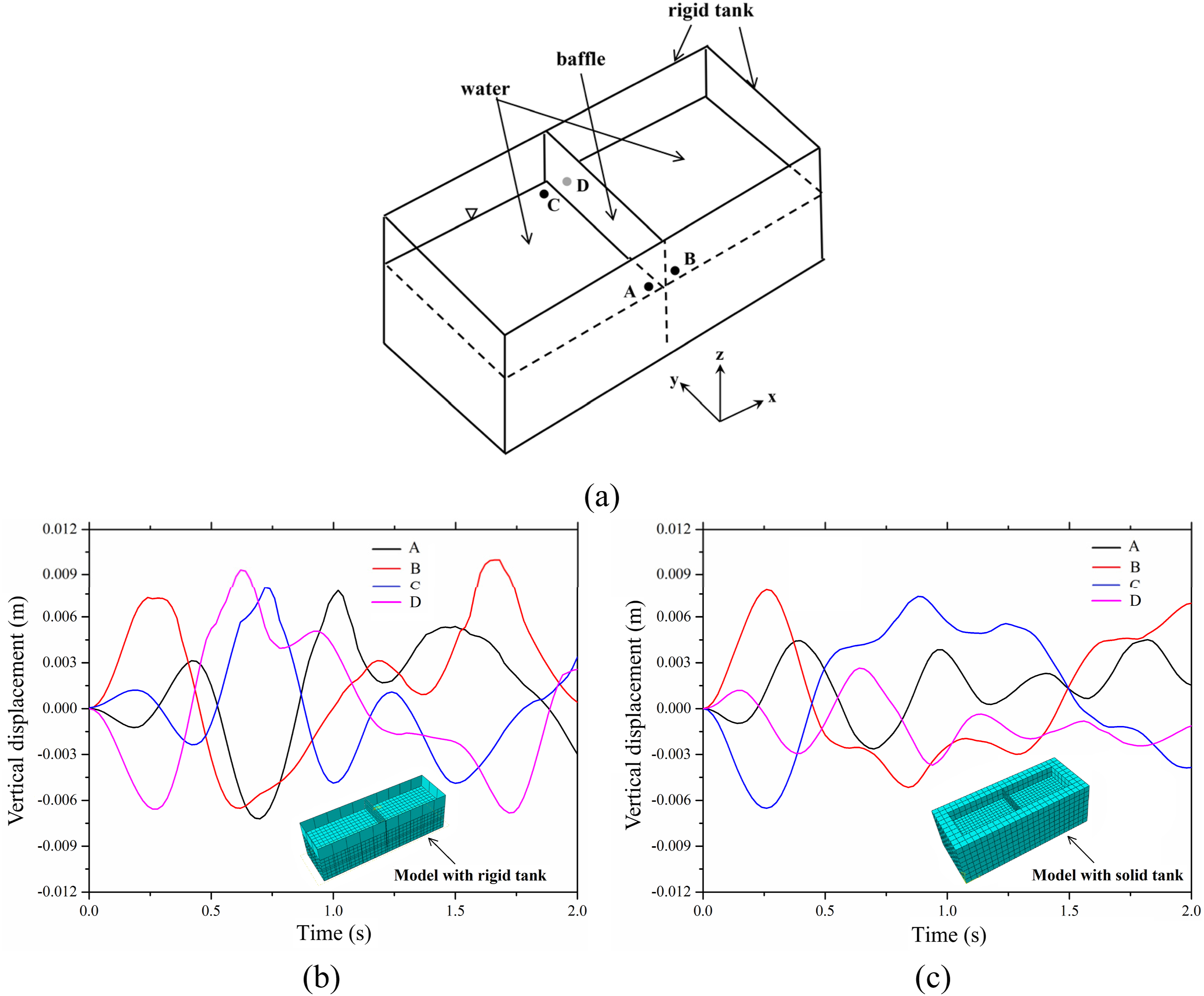

Parts	Model type	Density (kg/m³)	Model parameters
Solid tank	Elastic model	7850	Elastic modulus	Poisson's ratio
Solid tank	Elastic model	7850	20 GPa	0.3
Baffle	Mooney-Rivlin elastomeric model	10,901	Hyperelastic constant C₁₀	Hyperelastic constant C₀₁
Baffle	Mooney-Rivlin elastomeric model	10,901	689480 Pa	172370 Pa
Water	Newtonian viscous shear model and linear Us–Up equation	983	Wave speed	Shear viscosity
Water	Newtonian viscous shear model and linear Us–Up equation	983	45.85 m/s	0.0013 Pa·s

Figure 1(b) and (c) show the time histories of the vertical displacement of the water at the monitoring points. The vertical displacement trends at monitoring points of the model with the solid tank were similar to that of the ABAQUS example (model with a rigid tank), but the water sloshing amplitudes were smaller due to tank deformation. In summary, the results showed that the ALE method was suitable for solving fluid–structure interaction problems when the structures were modelled by solid elements, and it could be used for seismic response and isolation analyses of large-scale aqueducts.

Simplified model of frictional pendulum bearing

Frictional pendulum bearings (Zayas and Mahin, 1987) were placed between the aqueduct tank and the piers to improve the seismic performance of the aqueduct. According to the working mechanism of the frictional pendulum bearing, it can be regarded as a slider that makes a simple pendulum motion in a circular track. In this study, a simplified model that consisted of a simple pendulum (restoring force F_r) and a non-linear spring (friction force f) was used to model the frictional pendulum bearing (Wang et al., 2018), as shown in Figure 2(a). The simple pendulum can be considered to be a two-force rod with a length equal to the curvature radius of the sliding surface, and it was modelled by a linear elastic model. The elastic modulus of the simple pendulum should be taken to be a large value due to the very small vertical deformation of the frictional pendulum bearing. The non-linear spring was modelled by the ideal elastoplastic model with a large elastic modulus. The friction force f was the product of the vertical load applied to the slider and the friction coefficient for the actual model, while it was the product of the yield strength and the cross-sectional area of the non-linear spring for the simplified model.

Figure 2.

Validation of simplified model of frictional pendulum bearing: (a) schematic diagram of simplified model, and (b) comparison of test and simulation results.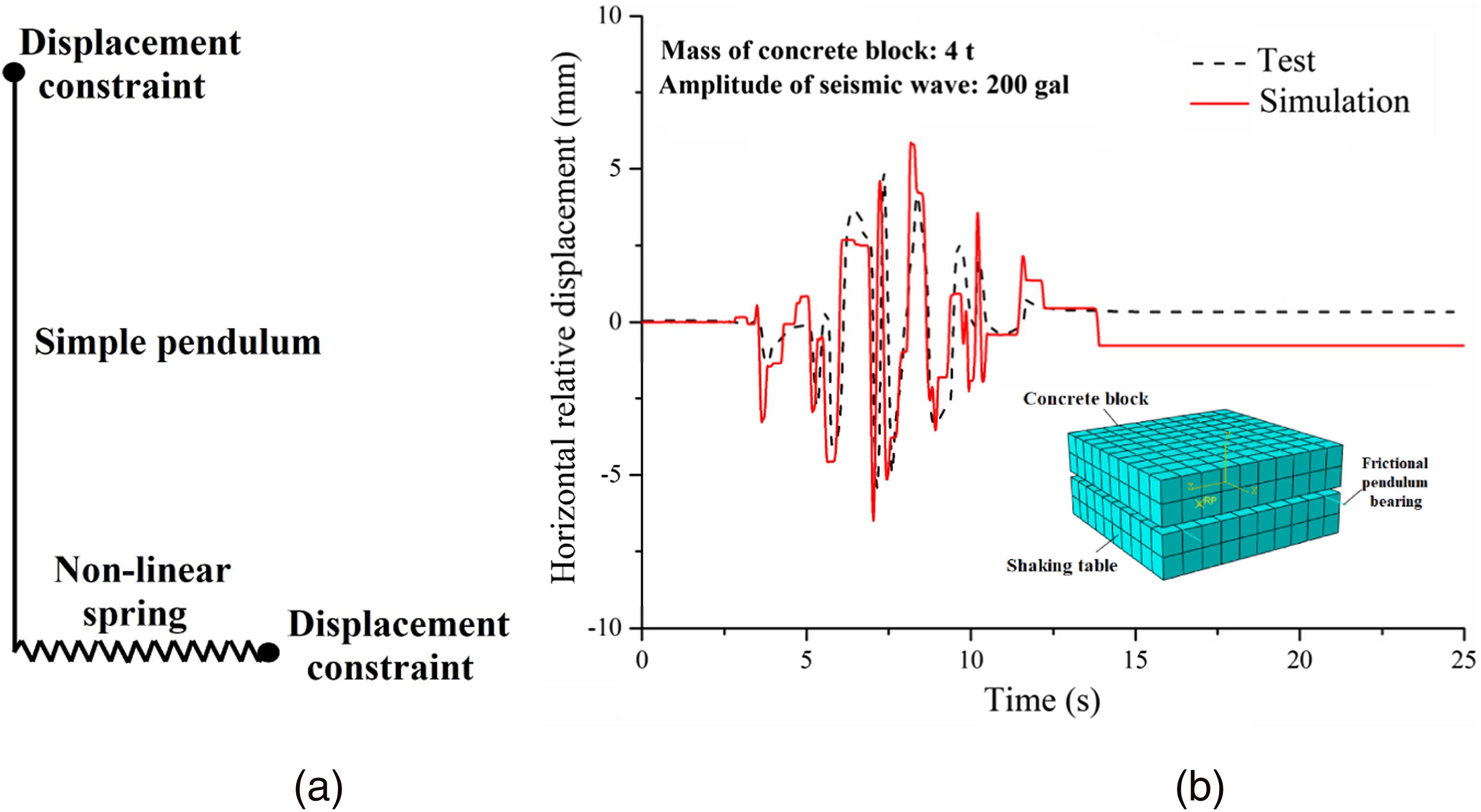

The simplified model was employed to simulate the shaking table tests conducted by Wang et al. (2018) to verify its validity, and the numerical model is shown in Figure 2(b). A Kobe seismic wave was used as the input motion with an amplitude of 200 or 250 gal, and the mass of concrete block was 4 or 6 t. Four frictional pendulum bearings with a friction coefficient of 0.06 were placed at the corners of the concrete block. The simple pendulum and non-linear spring were modelled using truss elements with linear elastic and ideal elastoplastic models, respectively. Their elastic moduli were 10⁸ and 9 × 10⁹ MPa, respectively. The length of the simple pendulum was 63 mm. The cross-sectional area of the non-linear spring was 0.05 m² and the yield strengths were 12 and 18 kPa corresponding to concrete block masses of 4 and 6 t, respectively. The comparisons of the simulation and test results are shown in Figure 2. It can be found that the simulation results were basically consistent with the test results, and the simplified model could well simulate the behaviour of the frictional pendulum bearing.

Pile–soil dynamic interaction model

Based on the Winkler foundation model, a combination of a linear elastic spring and a dashpot was used to simulate the pile–soil interactions under seismic loading (Gazetas et al., 1993) in this study. The elastic modulus of the spring was determined by the m method (Reese, 1965). The damping factor of the soil C consisted of material damping C_m and radiation damping C_r, which can be expressed as follows (Gazetas et al., 1993):

C_{m} = 2.0 ξ_{\max} (1 - \frac{G}{G_{\max}}) m ω,

(1)

C_{r} = 2 A \sqrt{G ρ_{s}} (1 + \frac{3.4}{π (1 - ν)}),

(2)

where ξ_max is the maximum damping ratio, which was calculated by the parameters of soil layers in this study, m is the modal effective mass of the soil, which was taken as the soil mass within the soil layer occupied by each pile in this study, ω is the first-order natural vibration frequency of the soil layer, A is the area of the soil layer occupied by each pile, G is the shear modulus, ρ_s is the density of soil, and υ is the Poisson's ratio of the soil. The validation of the dynamic Winkler foundation model was conducted by Gazetas et al. (1993) by comparing it with a rigorous method.

Viscoelastic artificial boundary

In practice, an aqueduct is connected to a water channel, but only the aqueduct section was modelled in this study. Therefore, the viscoelastic artificial boundaries at the two ends of the waterbody were required to simulate the actual water motion. A three-dimensional viscoelastic artificial boundary in the time domain proposed by Liu et al. (2006) was used in this study. A continuous spring–dashpot–lumped mass system was set up on the viscoelastic artificial boundary, and the stiffness of the spring K, damping of the dashpot C, and mass of the lumped mass M can be expressed as follows:

K = \frac{4 G}{R}, C = ρ c_{p}, M = ρ R,

(3)

where c_p is the P wave velocity of the media, R is the radial coordinate, G is the shear modulus, and ρ is the mass density of the medium.

In ABAQUS, Rayleigh damping is represented as a combination of the mass matrix [M] and the stiffness matrix [K] in the dynamical equations, as follows:

[C] = α [M] + β [K] .

(4)

Since the tangential behaviour of water is not considered, Rayleigh damping on the viscoelastic artificial boundary can be expressed as follows:

C = β K .

(5)

The stiffness factor is defined as follows:

K = \frac{E A}{L} = E h .

(6)

Therefore, the damping C can be expressed as follows:

C = ρ c_{p} = β E h .

(7)

In this study, ρ and c_p are the density and wave velocity of water, respectively, which are the same as those in Section 2.1. β is the Rayleigh damping factor of the boundary body with a value of 0.01. E is Young’s modulus of the boundary body with a value of 2 MPa. h is the depth of water, with a value of 5.0 m.

To verify the feasibility of the viscoelastic artificial boundary as well as determine its parameters, two tanks with a water depth of 1.0 m, Tank No. 1 and Tank No. 2, were established, as shown in Figure 3. The dimensions of Tank No. 1 and Tank No. 2 were 8 m × 4 m × 3 m and 20 m × 4 m × 3 m, respectively, and their thickness was 1 m. The viscoelastic artificial boundaries with a thickness of 45 mm were placed at the two ends along the length direction (x-direction) for Tank No. 1. The mesh size of viscoelastic artificial boundaries was close to that of water, which was about 15 × 15 × 14.5 mm. Viscoelastic artificial boundaries were not applied for Tank No. 2. The model parameters of the water and the tank were the same as those in Section 2.1, and a displacement pulse in the form of a sine wave with an amplitude of 0.05 m and a period of 2 s was prescribed for the tank in the x-direction. The comparison of the vertical displacement time histories for Tank No. 1 and Tank No. 2 is shown in Figure 3. It can be found that the results were basically consistent, and thus, the viscoelastic artificial boundary could be employed to simulate the free boundary of water motion.

Figure 3.

Verification of viscoelastic artificial boundary.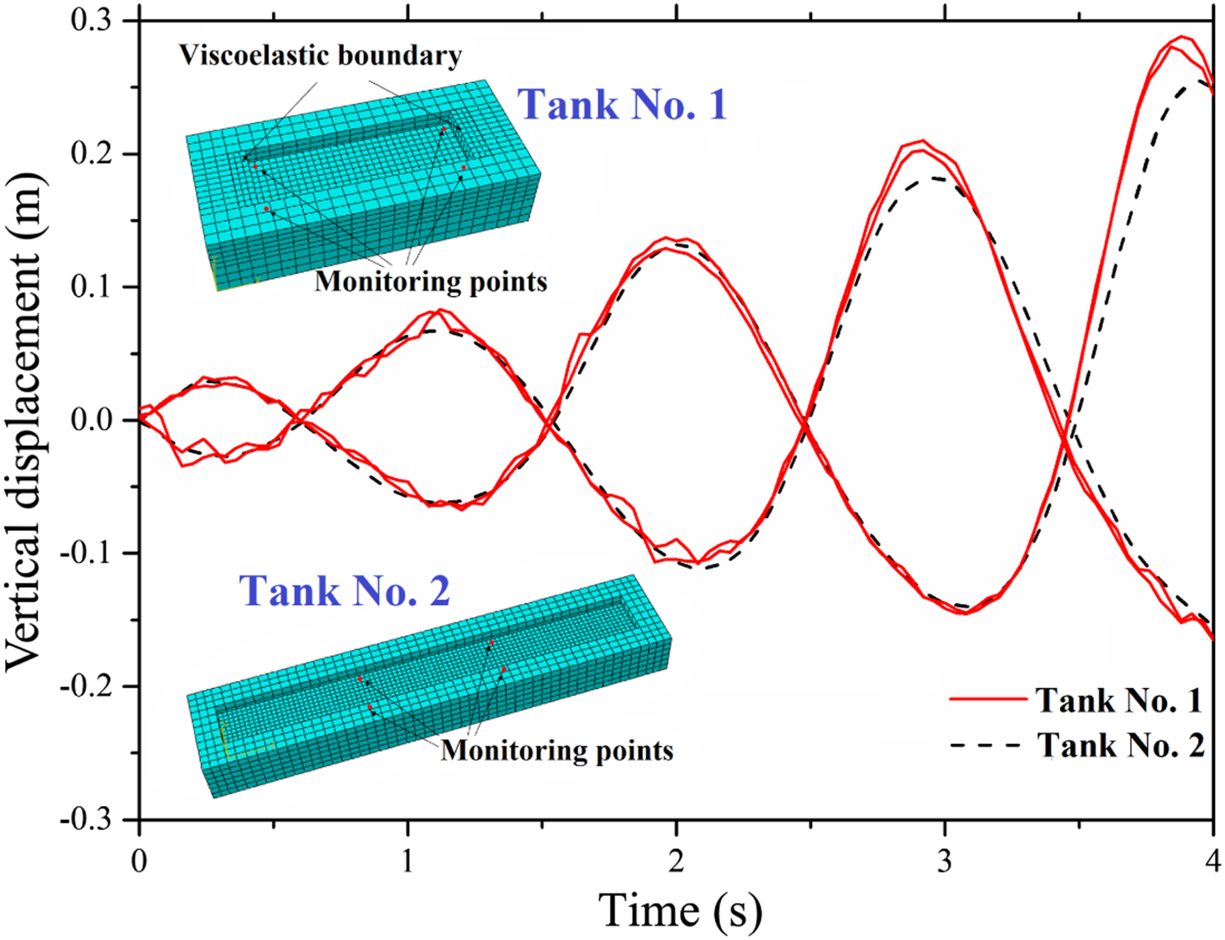

Numerical model

In this study, three types of three-dimensional finite element models, Model No. 1, Model No. 2, and Model No. 3, were established. Model No. 2 was the model with pile–soil dynamic interactions, which was used to investigate the seismic responses of the water–aqueduct structure–soil system. Model No. 1 and Model No. 3 were uniform and non-uniform seismic excitation models without considering pile–soil dynamic interactions, respectively, which were used to investigate the effects of pile–soil dynamic interactions and the seismic input method on the seismic response analysis of the large-scale aqueduct.

Aqueduct model

The elevation and cross sections of the whole aqueduct are shown in Figure 4, and the aqueduct tank with a whole length of 246 m and a width of 16 m consisted of three spans. The lengths of the side and middle spans were 68 and 110 m, respectively. The bridge decking of the aqueduct tank consisted of steel crossbeams and side baffles, and frictional pendulum bearings were installed under the two main trusses at each pier, as shown in Figure 4.

Figure 4.

Elevation and cross sections of the whole aqueduct (unit: cm).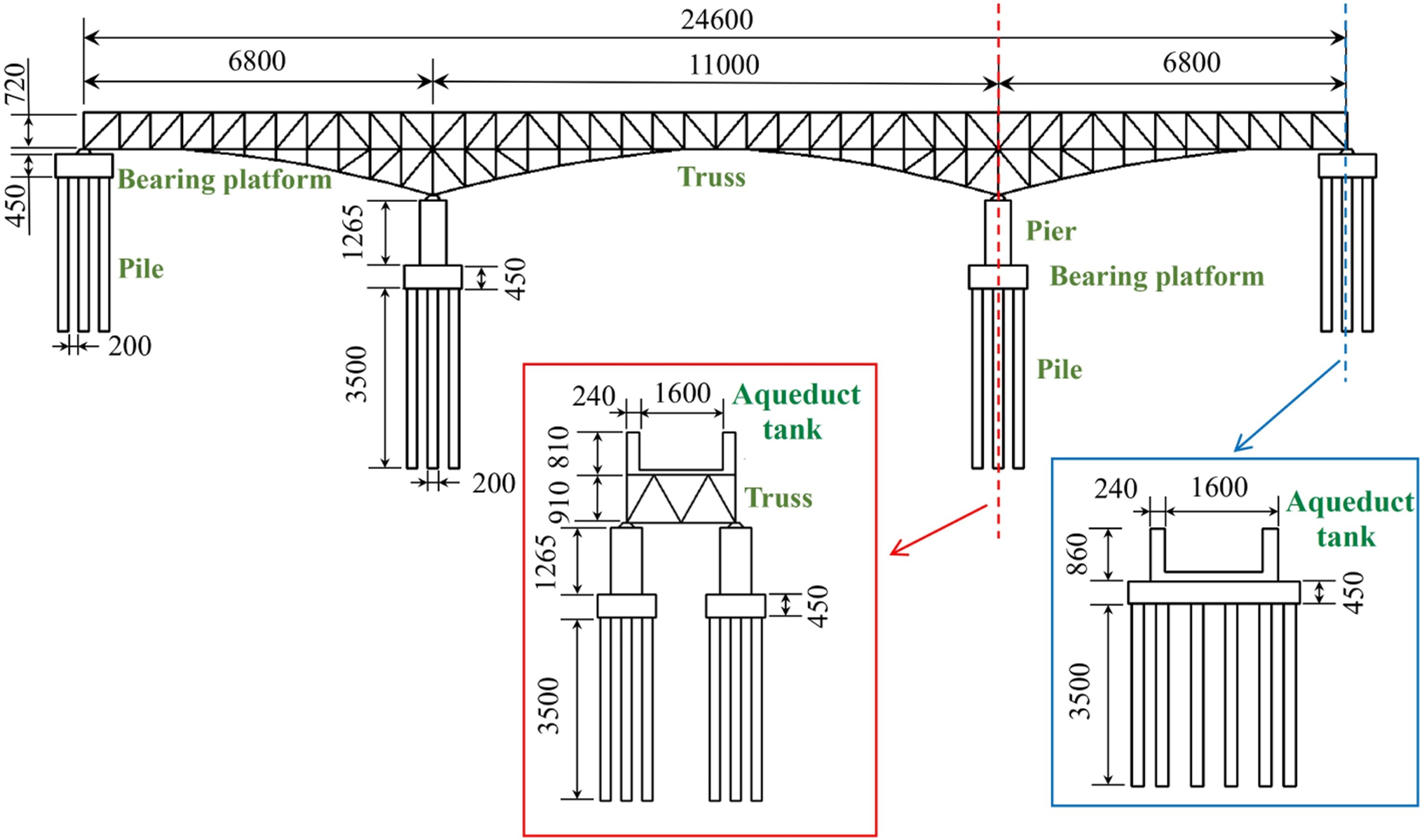

Two arched main trusses were set up transversely, and the aqueduct tank was placed between the two main trusses. The transverse width of the main truss was 1.5 m, and the centre distance of the two main trusses was 21.5 m. In addition, trussed crossbeams were installed near the middle piers to strengthen the transverse stiffness of the aqueduct tank, as shown in Figure 4. A self-balancing system was adopted in the aqueduct structure, and the thrust generated by the arch ribs was balanced by the lower chord of the main truss. Furthermore, there were pile group foundations on the bottom of the bearing platforms of the piers. The piles were fixed to bedrock with a diameter and length of 2 m and 35 m, respectively, as shown in Figure 4.

The numerical models of the whole aqueduct were established at a scale of 1:1 with the actual aqueduct, and the rebar cages were installed in piers and bearing platforms. Model No. 1 and Model No. 3 are shown in Figure 5(a), and Model No. 2 is shown in Figure 5(b). The only difference between Model No. 1 and Model No. 3 was the difference in the seismic input method. Uniform seismic excitation was adopted in Model No. 1, and the ground surface motion at the side pier was imposed on the bottom of the middle and side piers. However, non-uniform seismic excitation was adopted in Model No. 3, and the ground surface motions at the middle and side piers were imposed on the bottoms of the middle and side piers, respectively. Based on Model No. 1, Model No. 2 included added pile group foundations at the bottom of the middle and side piers, which were modelled by the pile–soil interaction model, and the bedrock ground motion was directly imposed at the bottom of the piles. The acquisitions of the ground surface motions and pile–soil interaction model parameters will be introduced in detail below.

Figure 5.

Numerical models of the whole aqueduct: (a) without pile–soil dynamic interactions (Model No. 1 and Model No. 3), and (b) with pile–soil dynamic interactions (Model No. 2).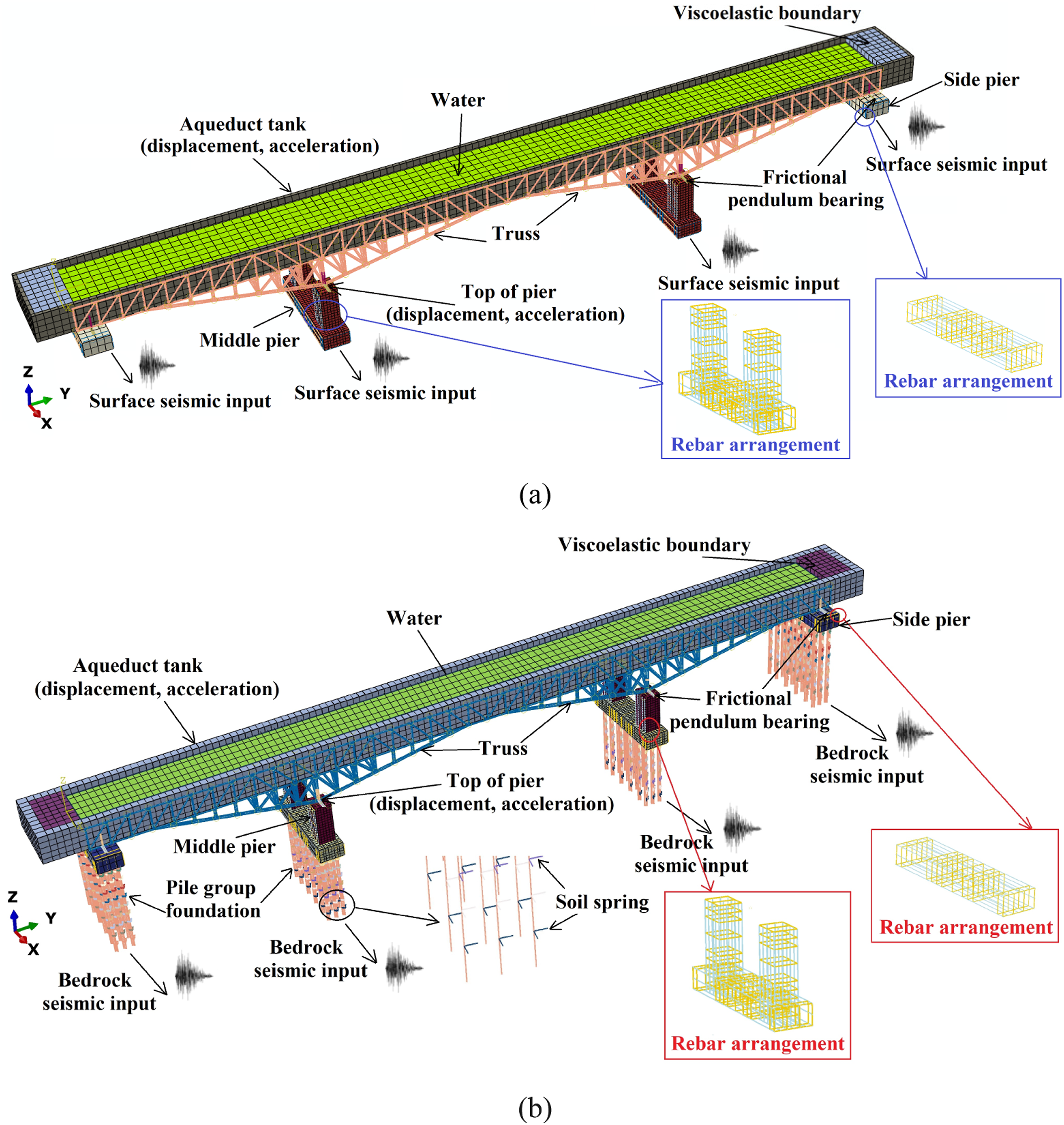

The model parameters of the aqueduct tank, pier, bearing platform, rebar, truss and beam are shown in Table 2. The cross-sectional area of the trusses was 0.12 m × 0.12 m, and the diameters of rebars and piles were 16 mm and 2 m, respectively. The model parameters of the water and the viscoelastic artificial boundary were the same as those in Sections 2.1 and 2.4, respectively. The depth of water was 5 m, which represented the full water condition. For the frictional pendulum bearing, the length of simple pendulum was 4 m, the cross-sectional area of the non-linear spring was 0.05 m², and the friction coefficient was 0.05. The eight bearings were subjected to an upper load of approximately 40,000 t, so the yield strength of the non-linear spring was 50,000 kPa.

Table 2.

Aqueduct model parameters.

Parts	Element type	Material	Density (kg/m³)	Elastic model
Parts	Element type	Material	Density (kg/m³)	Elastic modulus (GPa)	Poisson's ratio
Aqueduct tank	Solid	Steel	7850	210	0.3
Pier	Solid	C40 concrete	2400	33	0.2
Bearing platform	Solid	C50 concrete	2400	35	0.2
Longitudinal rebar	Truss	HRB400	7850	200	0.3
Transverse rebar	Truss	HPB300	7850	210	0.3
Truss	Beam	Steel	7850	210	0.3
Pile	Beam	C50 concrete	2400	35	0.2

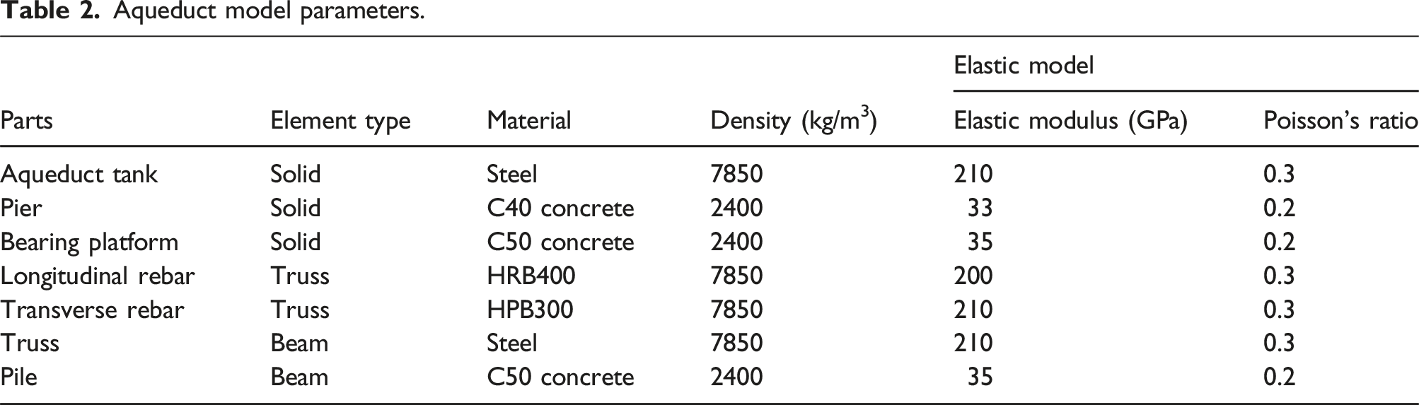
In this study, six seismic conditions were imposed on three types of models, i.e., two types of seismic motion (E1 and E2) with peak seismic accelerations of 0.24 g, 0.124 g, and 0.037 g, and the input seismic motions were introduced in the next subsection.

Input seismic motion

The two types of input seismic motion (E1 and E2) used in this paper were the horizontal ground motion perpendicular to the aqueduct direction at the bedrock, which were obtained from the seismic safety evaluation report of the Yangtze River–Huai River Water Diversion Project, as shown in Figure 6. The seismic motions with the peak seismic accelerations of 0.24 g, 0.124 g, and 0.037 g obtained by scaling from the original seismic motions were used to represent strong, moderate, and small earthquakes, respectively.

Figure 6.

Acceleration time histories of bedrock ground motion: (a) E1, and (b) E2.

For Model No. 2, the bedrock ground motion was directly imposed on the bottom of the piles. However, the pile–soil interactions were not considered in Model No. 1 and Model No. 3, and thus, the bedrock ground motion needed to be converted to ground surface motion and imposed on the bottom of the piers. In addition, it is worth noting that the ground surface motions at the middle and side piers were different due to the different thicknesses of the soil layers. The ground surface motions were obtained by one-dimensional seismic response analysis. The one-dimensional seismic response analysis involved the dynamic parameters of the soil layers which need to be determined first. Based on the engineering geological investigation report of the Pi River main canal aqueduct in the Yangtze River–Huai River Water Diversion Project, the properties of the soil layers at the aqueduct site were obtained, as shown in Table 3. The portion below soil layer No. 5 was bedrock.

Table 3.

Properties of soil layers.

Soil layer number	Soil type	Middle pier		Side pier		Density (kg/m³)
Soil layer number	Soil type	Thickness (m)	Shear wave speed (m/s)	Thickness (m)	Shear wave speed (m/s)	Density (kg/m³)
No. 1	Miscellaneous fill	3	140	3	148	1910
No. 2	Clay No. 1	3	233	9	257	2010
No. 3	Clay No. 2	6	266	9	295	2070
No. 4	Silty clay	3	276	0	—	2000
No. 5	Strongly weathered argillaceous sandstone	9	353	9	388	2050

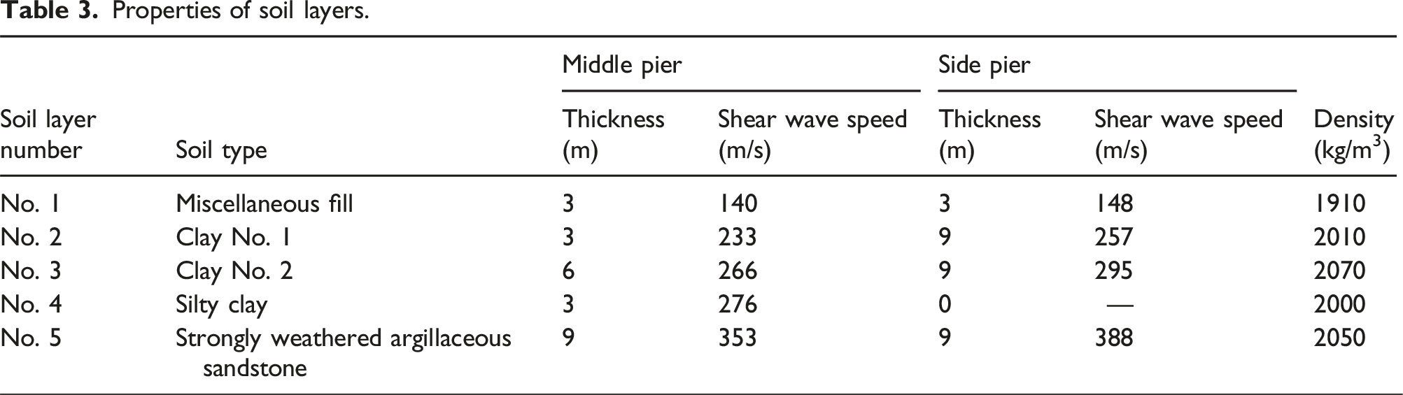
The Davidenkov model (Martin and Seed, 1982) was then employed to describe the dynamic stress–strain relationship in this study, which consisted of six parameters: the maximum shear modulus G_max, the maximum shear strain γ_max, Poisson’s ratio υ, and three model constants related to the soil dynamic properties, A, B, and γ₀. The G/G_max–γ and λ_d–γ relationships of five soil layers are shown in Figure 7. In addition, since the Davidenkov model was not available in ABAQUS, a subroutine of VUMAT-Davidenkov was compiled as a user-defined material function in ABAQUS to implement this model (Zhuang et al., 2007). The dynamic stress–strain relationship of the Davidenkov model is described as follows:

τ (γ) = G \cdot γ = G_{\max} \cdot γ \cdot [1 - H (γ)],

(8)

\frac{G}{G_{\max}} = 1 - H (γ) = 1 - {\frac{{(γ / γ_{0})}^{2 B}}{1 + {(γ / γ_{0})}^{2 B}}}^{A},

(9)

G_{\max} = {C_{s}}^{2} \cdot ρ_{s},

(10)

where C_s is the shear wave speed of the soil, and ρ_s is the density of soil. The parameters of A, B, and γ₀ were obtained from Figure 7, and the maximum shear strain γ_max was taken as 0.003 in this study. The Davidenkov model parameters of the five soil layers are shown in Table 4.

Figure 7.

Determination of soil dynamic parameters: (a) G/G_max–γ, and (b) λ_d–γ.

Table 4.

Davidenkov model parameters of soil layers.

Soil layer number	Thickness (m)		G_max (kPa)		υ	A	B	γ₀ (10⁻⁴)	γ _max
Soil layer number	Middle pier	Side pier	Middle pier	Side pier	υ	A	B	γ₀ (10⁻⁴)	γ _max
No. 1	3	3	37,436	41,837	0.35	4.17	0.32	0.15	0.003
No. 2	3	9	109,121	117,714	0.3	1.00	0.50	19.15	0.003
No. 3	6	9	158,829	168,136	0.3	1.00	0.50	19.55	0.003
No. 4	3	0	152,352	—	0.25	1.00	0.50	24.09	0.003
No. 5	9	9	296,020	280,645	0.2	1.00	0.50	19.67	0.003

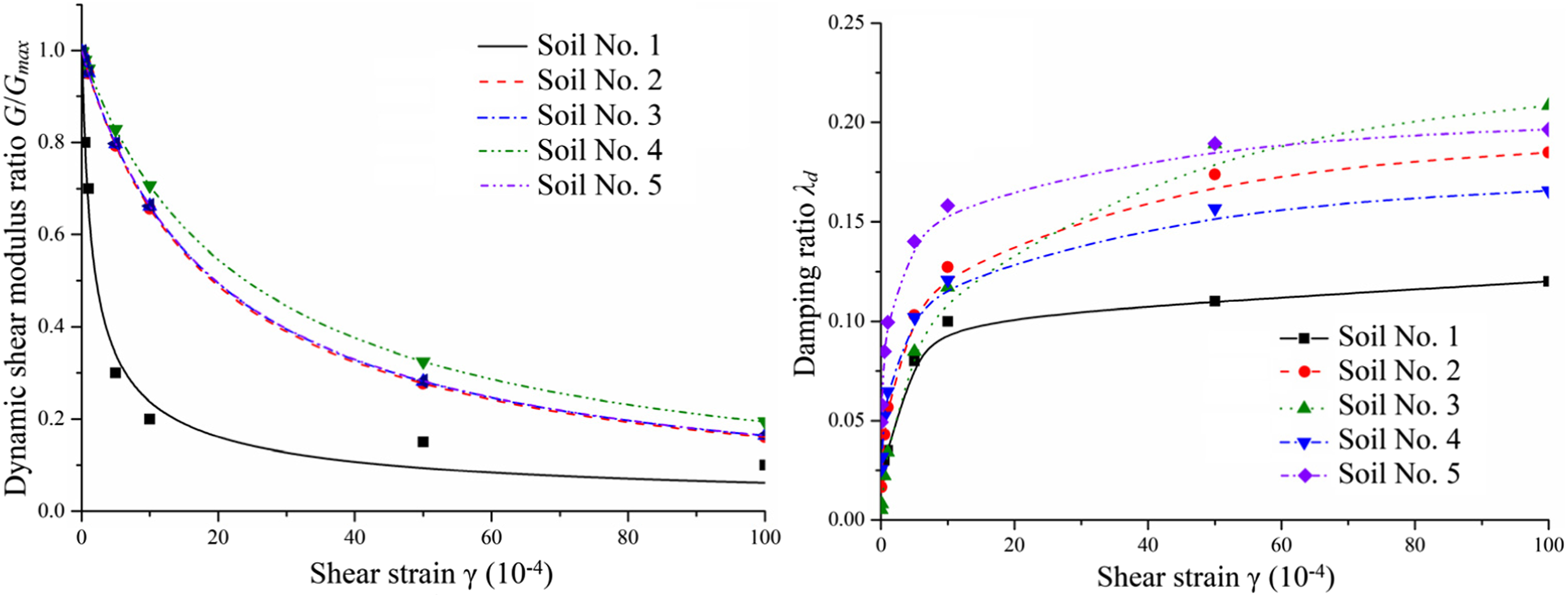
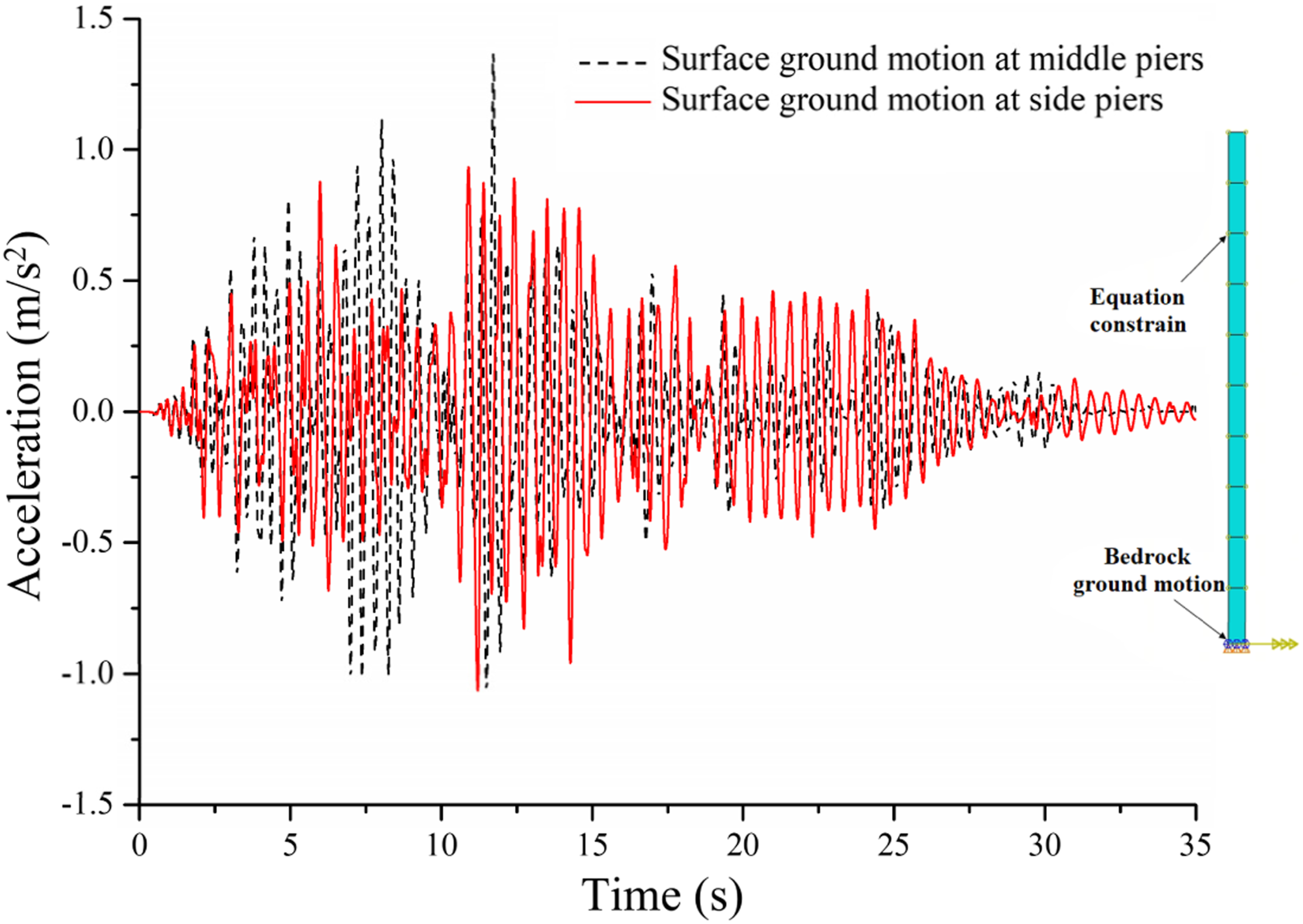
After obtaining the dynamic parameters of the soil layers, the dynamic shear strain and damping factors of the soil column needed to be determined. The side pier is discussed as an example to introduce the method in detail. First, the one-dimensional Davidenkov soil column model was established, and the dynamic parameters in Table 4 were assigned to the corresponding soil layers, as shown in Figure 8. The equation constraints were then added to the nodes of the soil layers to ensure that the nodes were always at the same level for each soil layer, and the acceleration time history of the bedrock ground motion was imposed at the bottom of the soil column. Finally, the time history of the horizontal relative displacement between the top and bottom nodes was exported, the ratio of the peak horizontal relative displacement to the soil layer thickness was taken as the maximum dynamic shear strain, and 0.65 times the maximum shear strain was taken as the equivalent shear strain. Based on the equivalent linearization model, the damping ratios of each soil layer were calculated by the following equations:

G = \frac{G_{\max}}{1 + γ / γ_{r}} \to \frac{G_{\max}}{G} = \frac{1}{γ_{r}} γ + 1,

(11)

λ = λ_{\max} {(1 - \frac{G}{G_{\max}})}^{M} \to \ln λ = M \ln (1 - \frac{G}{G_{\max}}) + \ln λ_{\max} .

(12)

Figure 8.

Acceleration time histories of ground surface motion.

The mass damping factor α and the stiffness damping factor β could be calculated by the following equations:

T = \sum \frac{4 L_{i}}{C_{s i}},

(13)

ω = \frac{2 π}{T},

(14)

α = 2 λ ω, β = \frac{2 λ}{ω},

(15)

where T is the first-order natural vibration period of the soil column, L_i is the thickness of ith soil layer, C_si is the shear wave speed of the ith soil layer, and ω is the first-order natural vibration frequency of the soil column.

The corresponding damping factors were assigned to the soils, and dynamic calculations were conducted on the soil column. The horizontal acceleration time histories at the top nodes of the soil column were exported as the ground surface motion at the side pier, and the ground surface motion at the middle pier was determined by a similar method. The acceleration time histories of the ground surface motions at the middle and side piers corresponding to the bedrock ground motion E1 with an amplitude of 0.037 g are shown in Figure 8.

Pile–soil interaction model parameters

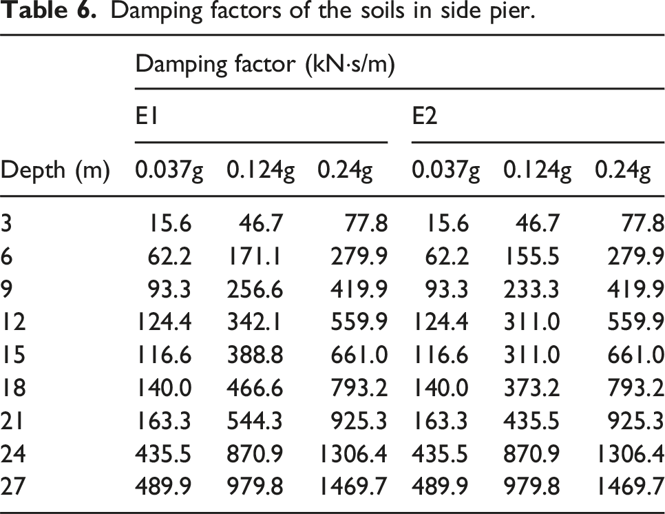
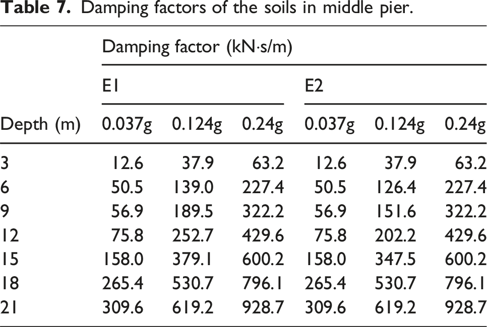
The pile–soil dynamic interactions were considered in Model No. 2, and the model parameters consist of three parts: the input displacements at the free end of the spring, elastic constant of the soil springs and damping factor of the soils. The input displacements at the free end of the spring were the time histories of the horizontal displacements at each soil layer node obtained from the one-dimensional seismic response analysis in the previous subsection.

The soil springs were modelled using truss elements, and the elastic constant k of the soil springs could be expressed as follows:

k = M y d_{0} l = 0.9 M y (d + l) l,

(16)

where M is the proportional coefficient of horizontal resistance with a value of 30,000 kN/m⁴ (JTG D63-2007, 2007), y is the embedded depth of the soil springs, d₀ [= 0.9(d + l)] is the representative value of the pile diameter, d is the diameter of the pile with a value of 2 m, and l is the length of the pile represented by the soil spring, which was 3 m in this study. The elastic constants of the soil springs at different depths can be found in Table 5.

Table 5.

Elastic constants of the soil springs.

Depth (m)		3	6	9	12	15	18	21	24	27
Elastic constant (kN/m)	Side pier	7776	15,552	23,328	31,104	38,880	46,656	54,432	62,208	69,984
Elastic constant (kN/m)	Middle pier	6318	12,636	18,954	25,272	31,590	37,908	44,226	—	—

The damping factor of the soil layers was the product of the spring constant and the stiffness damping factor β, and the acquisitions of the stiffness damping factors of soil layers have been introduced in the previous subsection. The damping factors of the soils in side and middle piers are shown in Tables 6 and 7.

Table 6.

Damping factors of the soils in side pier.

Depth (m)	Damping factor (kN·s/m)
	E1			E2
	0.037g	0.124g	0.24g	0.037g	0.124g	0.24g
3	15.6	46.7	77.8	15.6	46.7	77.8
6	62.2	171.1	279.9	62.2	155.5	279.9
9	93.3	256.6	419.9	93.3	233.3	419.9
12	124.4	342.1	559.9	124.4	311.0	559.9
15	116.6	388.8	661.0	116.6	311.0	661.0
18	140.0	466.6	793.2	140.0	373.2	793.2
21	163.3	544.3	925.3	163.3	435.5	925.3
24	435.5	870.9	1306.4	435.5	870.9	1306.4
27	489.9	979.8	1469.7	489.9	979.8	1469.7

Table 7.

Damping factors of the soils in middle pier.

Depth (m)	Damping factor (kN·s/m)
	E1			E2
	0.037g	0.124g	0.24g	0.037g	0.124g	0.24g
3	12.6	37.9	63.2	12.6	37.9	63.2
6	50.5	139.0	227.4	50.5	126.4	227.4
9	56.9	189.5	322.2	56.9	151.6	322.2
12	75.8	252.7	429.6	75.8	202.2	429.6
15	158.0	379.1	600.2	158.0	347.5	600.2
18	265.4	530.7	796.1	265.4	530.7	796.1
21	309.6	619.2	928.7	309.6	619.2	928.7

Numerical results

The simulation results are discussed in this section. Due to space restrictions, some results under seismic wave E2 that were similar to the results under seismic wave E1 are not presented.

Isolation effect of frictional pendulum bearings

In this study, the seismic isolation coefficient C_i was defined as the ratio of the peak horizontal accelerations of the superstructure and substructure connected to the bearing. The seismic isolation coefficients of the bearings at different positions under different seismic conditions are shown in Figure 9. The frictional pendulum bearings still provided a good seismic isolation effect despite the presence of water in the aqueduct tank. The seismic isolation effect of the bearing increased with increasing peak seismic acceleration and was better at the middle piers than at the side piers. In addition, the seismic isolation coefficients in the models without pile–soil interactions (Model No. 1 and Model No. 3) were smaller than those in the model with pile–soil interactions (Model No. 2), which means that the seismic isolation effect of frictional pendulum bearings may be overestimated if pile–soil interactions are not considered in finite element simulations.

Figure 9.

Seismic isolation coefficient under different seismic conditions.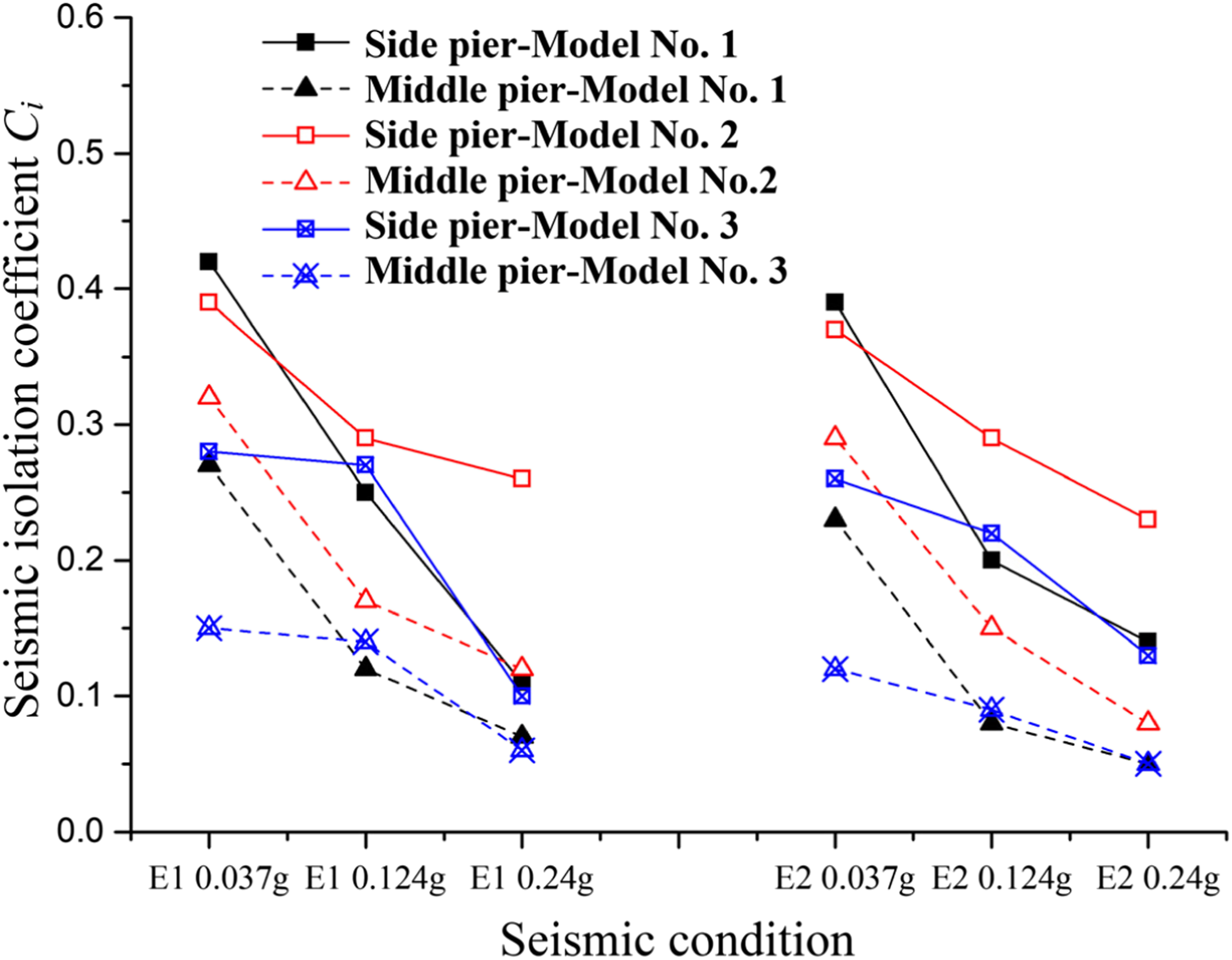

Horizontal deformation of frictional pendulum bearings

There may exist two damage modes for the aqueduct. One is the damage of the aqueduct tank due to excessive horizontal deflection at the mid-span location. The other is the damage of the frictional pendulum bearing due to excessive relative displacement between the aqueduct tank and the piers. The relative slip between the aqueduct tank and the piers and the deformation of the aqueduct tank at the mid-span are shown in Figure 10(a) and (b), respectively. It can be found that the horizontal deflection of the aqueduct tank at the mid-span was small due to the restraint of the main trusses, and the relative displacement between the aqueduct tank and the piers was relatively large, which could lead to large deformation of the friction pendulum bearing and an additional internal force response in the piers.

Figure 10.

Deformation diagram of the aqueduct: (a) relative slip between aqueduct tank and piers (magnification 20 times), and (b) deformation of aqueduct tank at mid-span (magnification 100 times).

Figure 11 shows the horizontal deformation time histories of bearings under seismic wave E1. The responses of the bearings at middle and side piers in Model No. 1 were similar due to the uniform seismic excitation. As shown in Figure 11(a)–(c), the bearing deformations at the middle pier in Model No. 1 and Model No. 2 were similar, but the bearing deformation at the side pier in Model No. 1 was smaller than that in Model No. 2. This means that the horizontal deformation of the frictional pendulum bearing at the side pier may be underestimated if pile–soil interactions are not considered in the finite element simulation.

Figure 11.

Horizontal deformation time histories of bearings: (a) middle pier of Model No. 1, (b) middle pier of Model No. 2, (c) side pier of Model No. 2, and (d) Model No. 3.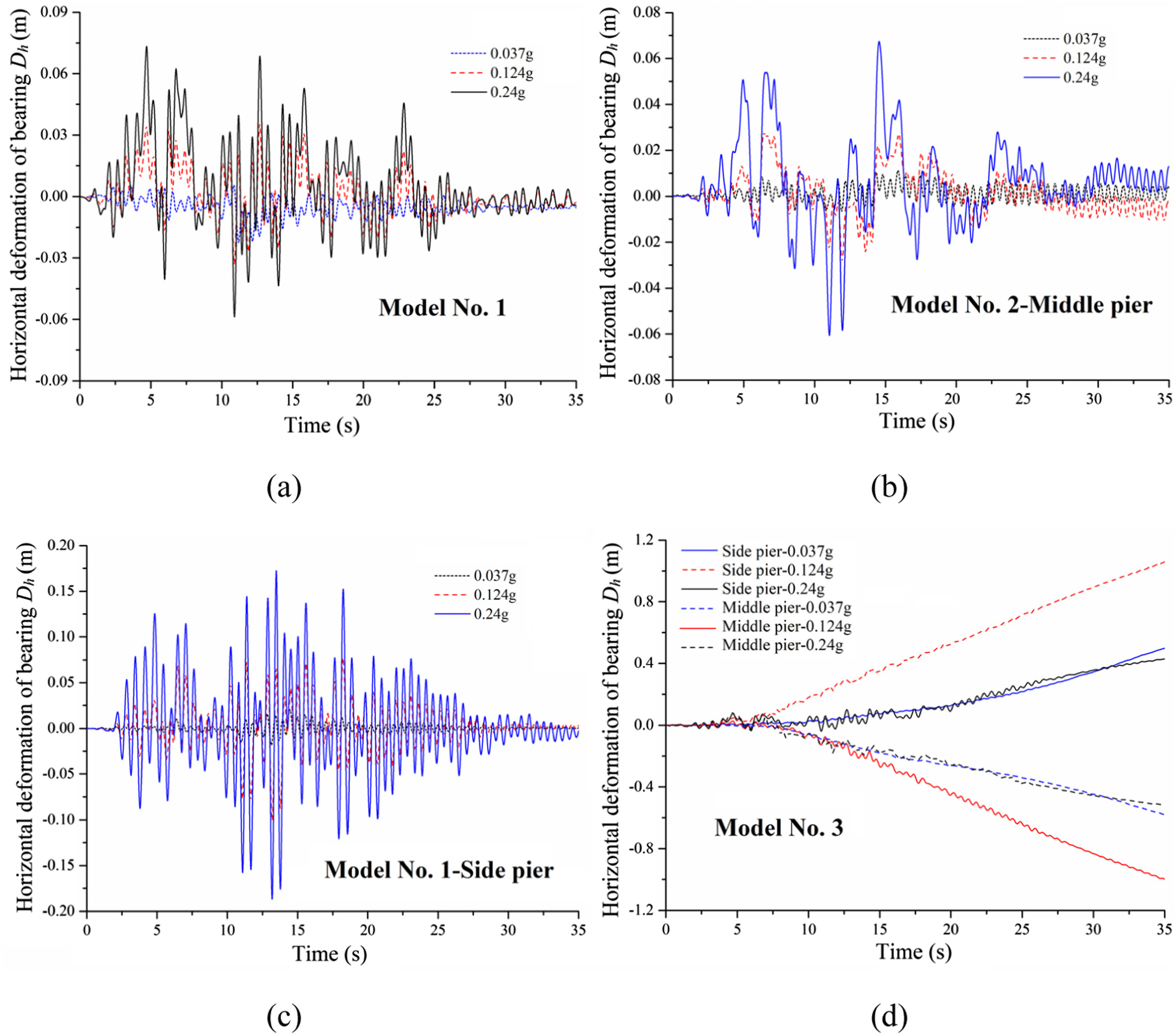

In addition, Figure 11(d) shows that the bearing deformations in Model No. 3 were extremely large and increased significantly with time. However, it is impossible for the bearings to deform this much in practice, which means that the non-uniform seismic excitation model (Model No. 3) is not suitable for analysing the seismic responses of large-scale aqueducts.

Relative horizontal displacement and stress distribution of middle piers

Figure 12 shows the peak horizontal relative displacement between the top and bottom of the middle pier under different seismic conditions. It can be found that the peak horizontal relative displacement increased with increasing peak seismic acceleration. The uniform seismic excitation model (Model No. 1) may have underestimated the peak horizontal relative displacement due to the lack of consideration of the non-uniformity of the seismic waves imposed on the piers, and the non-uniform seismic excitation model (Model No. 3) may have overestimated the peak horizontal relative displacement due to the lack of consideration of the restraint effect of the piles and soil on the superstructure.

Figure 12.

Peak horizontal relative displacements of middle piers.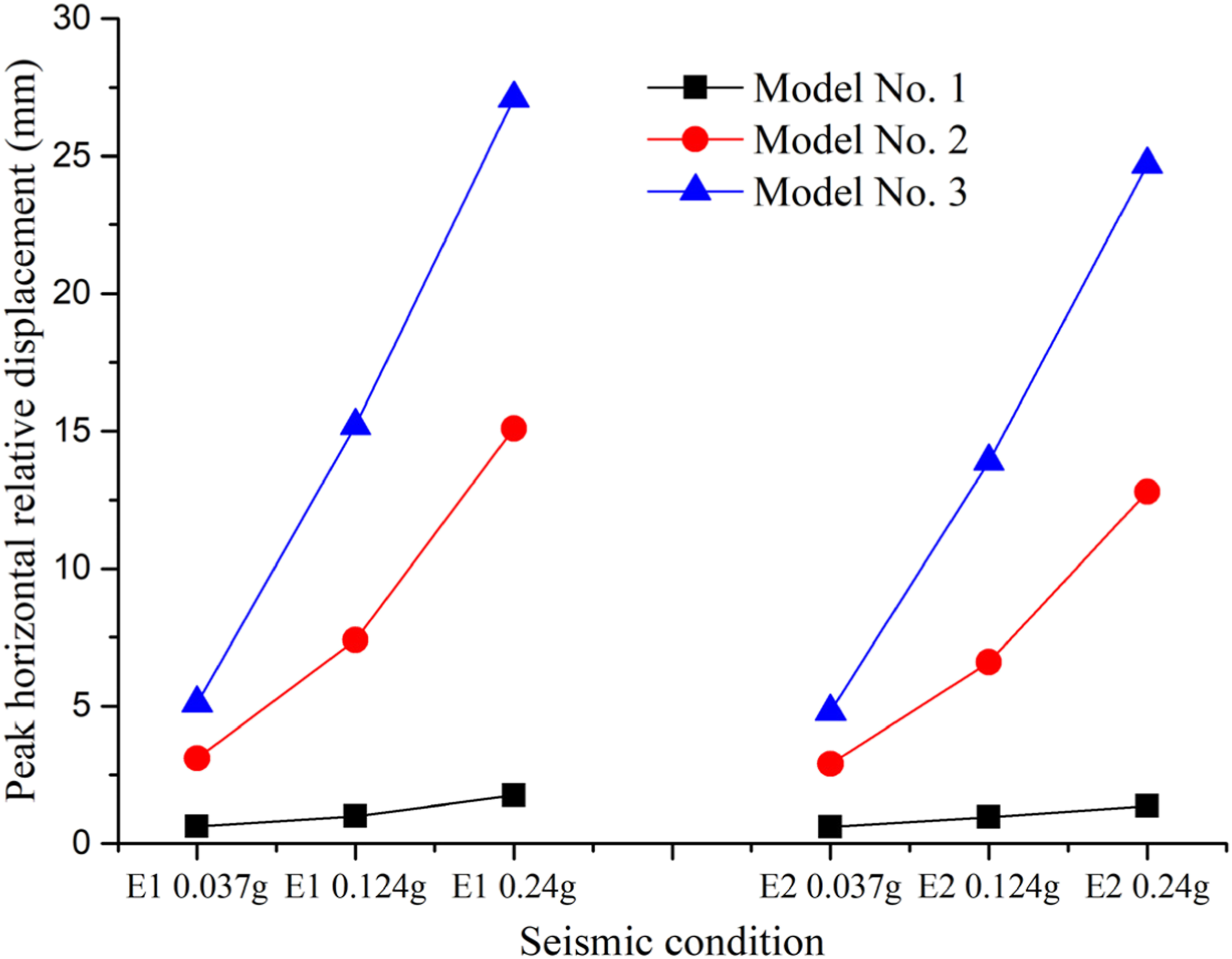

Figure 13 shows the stress cloud diagrams of the middle piers under the most dangerous condition. It can be found that the maximum tensile, compressive, and shear stresses were mainly distributed in the corners of the middle piers, and Model No. 1 and Model No. 3 also underestimated and overestimated the maximum stresses of the middle piers, respectively, due to reasons similar to those mentioned above.

Figure 13.

Stress cloud diagrams of the middle piers.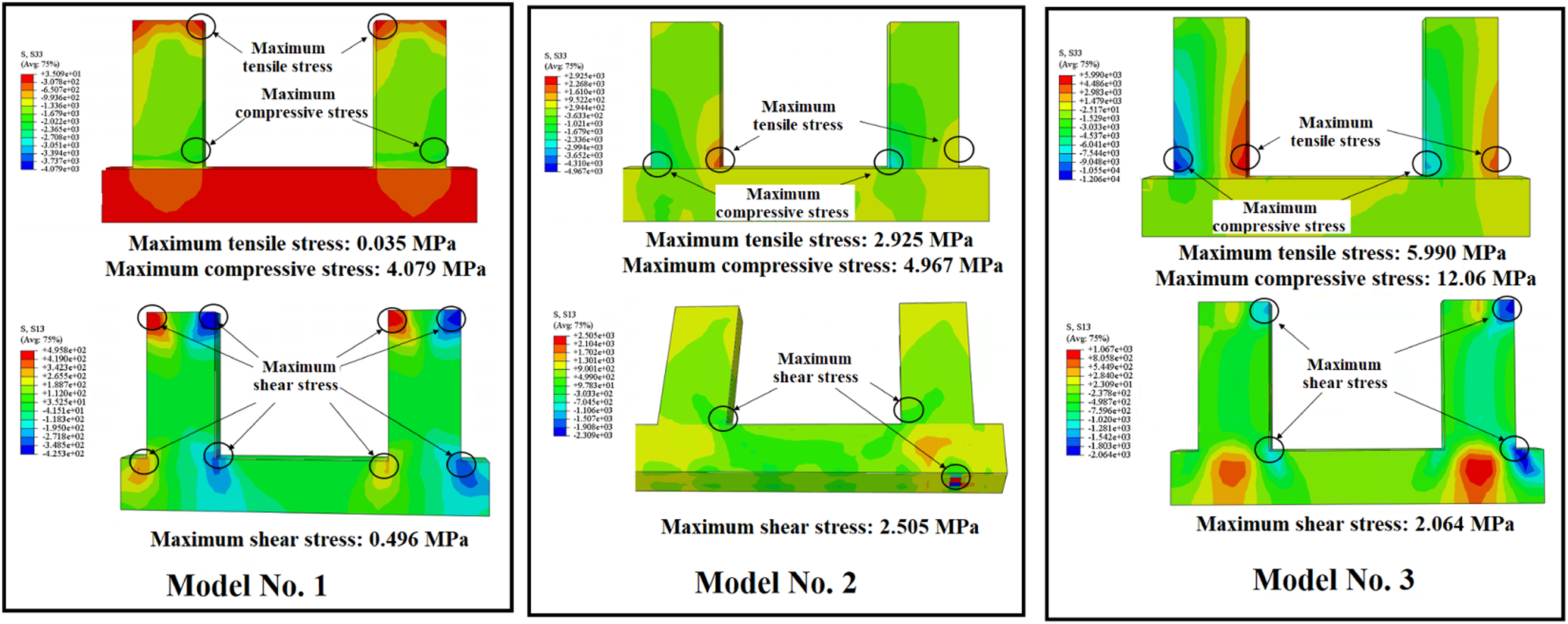

The maximum compressive and shear stresses of the middle pier in Model No. 2 were 5.0 and 2.51 MPa, respectively, which were smaller than the compressive strength (26.8 MPa) and shear strength (3.5 MPa) of concrete. However, the maximum tensile stress of the middle pier in Model No. 2 was 2.925 MPa, which was slightly larger than the tensile strength (2.39 MPa) of concrete. Therefore, the tensile strength of concrete at the pier corners needed to be enhanced to ensure the safety of the whole aqueduct.

Water sloshing

Figure 14 shows the vertical displacement time history of water at the mid-span under seismic wave E1. The water sloshing was relatively stable with good consistency along the aqueduct direction. The amplitude increased, but the frequency was basically unchanged with increasing peak seismic acceleration. In addition, the trends of water sloshing in Model No. 1 and Model No. 2 were basically the same, with only slightly larger amplitudes in Model No. 2.

Figure 14.

Vertical displacement time history of water at mid-span: (a) Model No. 1, and (b) Model No. 2.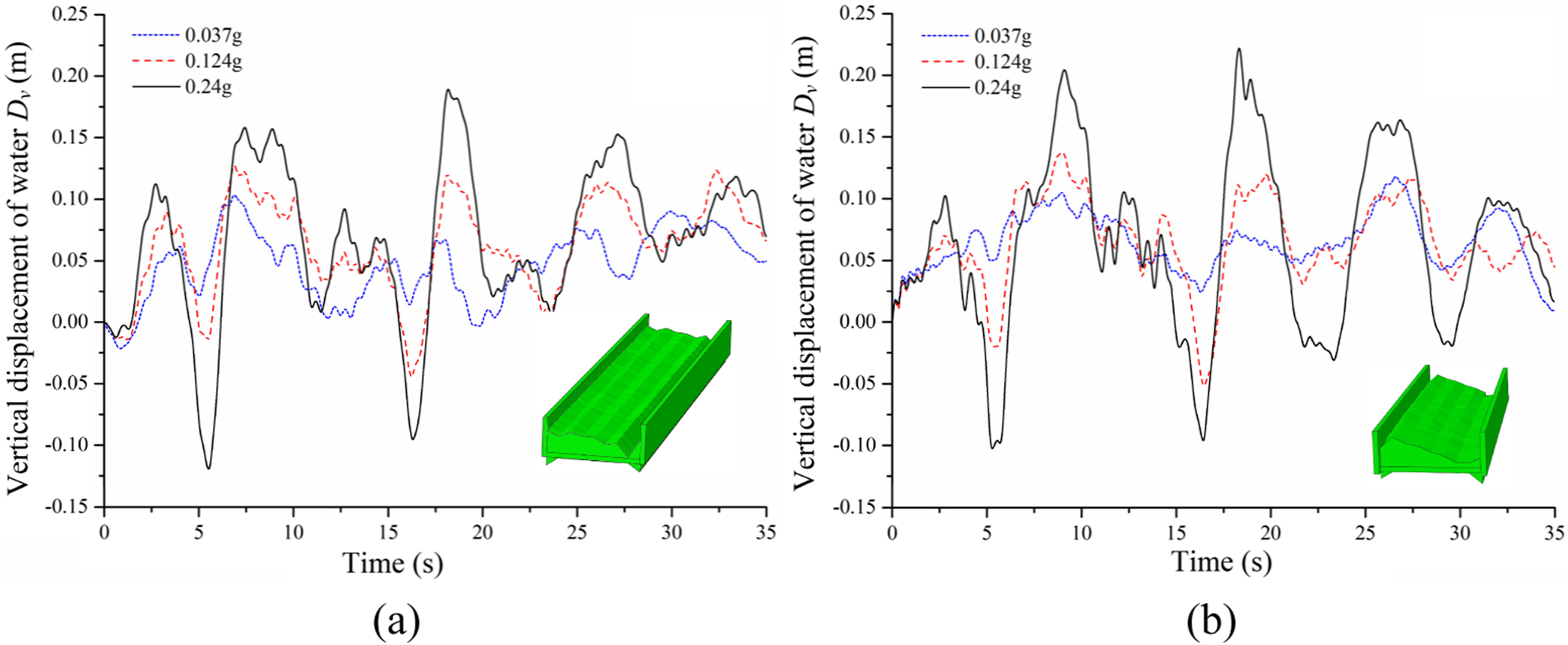

Figure 15 shows the maximum water pressure at the bottom of aqueduct sidewall under seismic conditions, including hydrostatic and hydrodynamic pressure. It can be found that the maximum water pressure increased with increasing peak seismic acceleration, and was larger in Model No. 2 than in Model No. 1.

Figure 15.

Maximum water pressure at the bottom of aqueduct sidewall.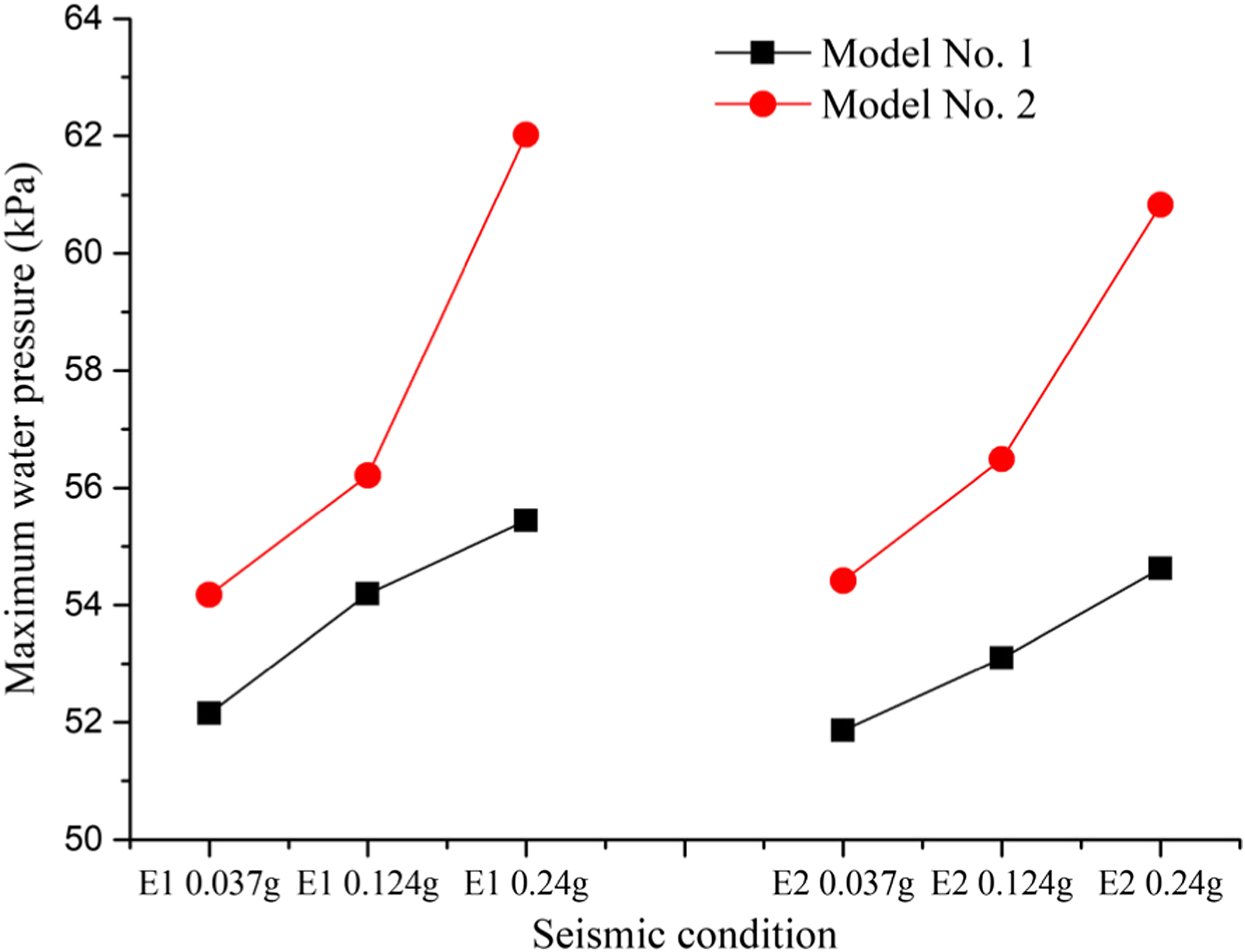

In summary, since the non-uniformity of the seismic waves imposed on the piers was not considered, the uniform seismic excitation model (Model No. 1) overestimated the seismic isolation effect of the frictional pendulum bearing and underestimated the horizontal deformation of the frictional pendulum bearing, the peak horizontal relative displacement and maximum stresses of the middle pier, and the amplitude of water sloshing. Furthermore, although the non-uniform seismic excitation model (Model No. 3) could reflect the non-uniformity of the seismic waves imposed on the piers due to the field effect, the simulation results were unrealistic due to the lack of consideration of the restraint effect of the pile and soil on the superstructure. Therefore, it is necessary to consider the pile–soil dynamic interactions in the seismic response analysis of large-scale aqueducts.

Conclusions

In this study, large-scale aqueduct models with and without the consideration of pile–soil dynamic interactions were established, and the differences in the dynamic responses of these models under earthquake loading were compared. Based on the numerical results, the major findings are summarized as follows:

(1) The uniform seismic input analysis without considering the pile–soil dynamic interactions might result in a small dynamic response, while a non-uniform seismic excitation directly imposed to the piers might result in an unrealistic dynamic response. Therefore, it is necessary to consider the dynamic interactions of the pile–soil–aqueduct structure in the seismic analysis of large-scale aqueducts.

(2) The frictional pendulum bearings still provided a good seismic isolation effect despite the presence of water in the aqueduct tank. The seismic isolation effect of the bearing increased with increasing peak seismic acceleration and was better at the middle piers than at the side piers.

(3) The maximum tensile, compressive, and shear stresses of the middle piers were mainly distributed in the corners, and there was a risk of tensile damage to the middle piers under earthquake loads. Therefore, it is necessary to enhance the tensile strength of concrete at the pier corners to ensure the safety of aqueducts.

To improve the computational efficiency of the model, an elastic model was adopted to simulate the concrete behaviour, the soil was simplified as springs and dashpots, and the frictional pendulum bearings were simplified as simple pendulums and springs in this study, which may have reduced the simulation accuracy. More reliable results may be obtained by using the concrete damage plasticity model and by modelling the soil and bearings as solid elements.

Footnotes

Author contributions

Yuting Zhang: Conceptualization, Writing – review & editing. Yinjie Peng: Software, Writing – original draft. Shusheng Qu: Writing – review & editing. Huabei Liu: Supervision, Validation, Writing – review & editing. Kaifeng Zeng: Visualization, Writing – original draft, Writing – review & editing.

Declaration of conflicting interests

The authors declared no potential conflicts of interest with respect to the research, authorship, and/or publication of this article.

Funding

The authors disclosed receipt of the following financial support for the research, authorship, and/or publication of this article: This study was supported by the Fundamental Research Funds for the Central Public Welfare Research Institutes (No. TKS20240401), which is gratefully acknowledged.

ORCID iD

Kaifeng Zeng

Data Availability Statement

All the data, model or code data employed in the study can be available on reasonable request from the corresponding author.*

References

Chen

Jiang

Tao

, et al. (2012) Seismic response analysis of high-speed vehicle-bridge considering soil-structure interaction. Rock and Soil Mechanics 33(10): 3162–3170, (in Chinese).

Dassault Systemes Simulia Corp. (DSS) (2014) ABAQUS 6.14 online documentation.

Gazetas

Makris

(1991) Dynamic pile-soil-pile interaction. Part I: analysis of axial vibration. Earthquake Engineering and Structural Dynamics 20(2): 115–132.

Gazetas

Fan

Kaynia

(1993) Dynamic response of pile groups with different configurations. Soil Dynamics and Earthquake Engineering 12(4): 239–257.

GB51247-2018 (2018) Standard for Seismic Design of Hydraulic Structures. Beijing: China Planning Press. (in Chinese).

Hirt

Amsden

Cook

(1974) An arbitrary Lagrangian-Eulerian computing method for all flow speeds. Journal of Computational Physics 14: 227–253.

Housner

(1957) Dynamic pressures on accelerated fluid containers. Bulletin of the Seismological Society of America 47(1): 15–35.

JTG D63-2007 (2007) Specifications for Design of Ground Base and Foundation of Highway Bridges and Culverts. Beijing: China Communication Press. (in Chinese).

Kildashti

M Dolatshahi

Mirghaderi

(2016) A case study on the soil–pile–structure interaction of a long span arched structure. Structure and Infrastructure Engineering 12(12): 1614–1633.

10.

Kim

Chang

Yun

(2002) Fluid-structure-soil interaction analysis of cylindrical liquid storage tanks subjected to horizontal earthquake loading. Structural Engineering and Mechanics 13(6): 615–638.

11.

Lou

Pan

(2003) Evaluation of vertical seismic response for a large-scale beam‐supported aqueduct. Earthquake Engineering & Structural Dynamics 32(1): 1–14.

12.

Wan

Zhao

, et al. (2021) Three-Dimensional analysis of nonlinear pile-soil interaction responses using 3D pile element model. International Journal of Geomechanics 21(8): 04021129.

13.

Liu

, et al. (2006) 3D viscous-spring artificial boundary in time domain. Earthquake Engineering and Engineering Vibration 5(1): 93–102.

14.

Luo

Yang

Zhan

, et al. (2016) Nonlinear 3D finite element analysis of soil-pile-structure interaction system subjected to horizontal earthquake excitation. Soil Dynamics and Earthquake Engineering 84: 145–156.

15.

Maheshwari

Truman

El Naggar

, et al. (2004) Three-dimensional nonlinear analysis for seismic soil–pile-structure interaction. Soil Dynamics and Earthquake Engineering 24(4): 343–356.

16.

Makris

Gazetas

(1992) Dynamic pile-soil-pile interaction. Part II: lateral and seismic response. Earthquake Engineering and Structural Dynamic 21(2): 145–162.

17.

Martin

Seed

(1982) One-dimensional dynamic ground response analyses. Journal of the Geotechnical Engineering Division 108(7): 935–952.

18.

Nakayama

Washizu

(1981) The boundary element method applied to the analysis of two-dimensional non-linear sloshing problems. International Journal for Numerical Methods in Engineering 17(11): 1631–1646.

19.

Novak

(1974) Dynamic stiffness and damping of piles. Journal of Canadian Geotechnical 11(4): 574–598.

20.

Novak

Aboul-Ella

Nogami

(1978) Dynamic soil reactions for plane strain case. Journal of the Engineering Mechanics Division 104(4): 953–959.

21.

Reese

(1965) Non-dimensional solution for laterally loaded piles with soil modulus assumed proportional to depth. Austin, TX, USA: The University of Texas.

22.

Soneji

Jangid

(2008) Influence of soil–structure interaction on the response of seismically isolated cable-stayed bridge. Soil Dynamics and Earthquake Engineering 28(4): 245–257.

23.

Song

Yang

Jia

, et al. (2023) Seismic response and instability analysis of the liquefiable soil-piles-superstructure interaction system. Structures 54: 134–152.

24.

Valeti

Ray-Chaudhuri

Raychowdhury

(2016) Seismic response of an elevated aqueduct considering hydrodynamic and soil-structure interactions. International Journal of Advanced Structural Engineering 8: 53–71.

25.

Wang

Feng

(2018) A simplified simulation method of friction pendulum bearings. Journal of Southeast University 34(4): 480–487.

26.

Westergarrd

(1933) Water pressures on dams during earthquakes. Transactions of American Society of Civil Engineering 98: 418–433.

27.

Zhang

, et al. (2023) Overall seismic reliability analysis of aqueduct structure based on different levels under random earthquake. Structures 58: 105469.

28.

Xiao

Yang

Zhuang

, et al. (2021) A numerical and theoretical analysis of the structural performance for a new type of steel-concrete composite aqueduct. Engineering Structures 245: 112839.

29.

Liu

Jiang

, et al. (2021) Dynamic damage mechanism and seismic fragility analysis of an aqueduct structure. Applied Sciences 11(24): 11709.

30.

Zayas

Mahin

(1987) The FPS Earthquake Resisting System Experimental Report. Berkeley, CA: Earthquake Engineering Research Center.

31.

Zhang

Sun

Liu

, et al. (2013a) Resonance mechanism of wind-induced isolated aqueduct-water coupling system. Engineering Structures 57: 73–86.

32.

Zhang

Liu

Dong

, et al. (2013b) Analysis of wind-induced vibration of fluid–structure interaction system for isolated aqueduct bridge. Engineering Structures 46: 28–37.

33.

Zhang

Qian

, et al. (2022a) Seismic reliability analysis of random parameter aqueduct structure under random earthquake. Soil Dynamics and Earthquake Engineering 153: 107083.

34.

Zhang

Wang

, et al. (2022b) Fragility analysis of high-span aqueduct structure under near-fault and far-field ground motions. Structures 46: 681–697.

35.

Zhuang

Chen

Liang

, et al. (2007) A developed dynamic viscoelastic constitutive relations of soil and implemented by ABAQUS software. Rock and Soil Mechanics 28(3): 436–442, (in Chinese).

Seismic response of a large,isolated aqueduct considering fluid–structure and soil–structure interactions

Abstract

Keywords

Introduction

Description of numerical approach

Arbitrary Lagrangian–Eulerian (ALE) fluid–structure interaction model

Simplified model of frictional pendulum bearing

Pile–soil dynamic interaction model

Viscoelastic artificial boundary

Numerical model

Aqueduct model

Input seismic motion

Pile–soil interaction model parameters

Numerical results

Isolation effect of frictional pendulum bearings

Horizontal deformation of frictional pendulum bearings

Relative horizontal displacement and stress distribution of middle piers

Water sloshing

Conclusions

Footnotes

Author contributions

Declaration of conflicting interests

Funding

ORCID iD

Data Availability Statement

References