Numerical calculation of bridge temperature considering all-weather conditions

Abstract

Temperature is one of the critical environmental factors affecting bridges’ performance. Accurate temperature distribution is essential for reliable structural condition assessment. Existing studies have predominantly focused on the most adverse thermal conditions under clear skies, but seldom considered the cloudy or rainy conditions, which may not reflect the actual scenario of the bridges in real-time structural monitoring. This study develops a numerical method to calculate the bridge temperature distribution under all-weather conditions, including sunny, cloudy, rainy, and snowy scenarios. According to the illuminance and cloud cover, real-time solar radiation correction models are employed to quantify the shielding effect of clouds on solar radiation during cloudy or rainy weather. These models, combined with other meteorological parameters such as air temperature and wind speed, enable accurate determination of thermal boundary conditions for refined heat-transfer analysis. An automatic computational framework is strategically developed for weather scenario classification, boundary condition determination, and heat-transfer analysis. The proposed framework is applied to three scenarios: An experimental reinforced concrete slab, a practical steel box girder suspension bridge, and a real concrete box girder continuous bridge. Results demonstrate that the proposed correction models significantly enhance the heat-transfer analysis accuracy under various weather conditions. A good agreement has been achieved between simulated and measured temperatures across girder sections with different materials and geometries, thereby verifying the effectiveness of the proposed method. This study establishes a theoretical foundation and practical framework for investigating bridge temperature behaviors under complex weather conditions.

Keywords

temperature field heat-transfer analysis numerical simulation cloud condition bridge structure

Introduction

Exposed to natural environments, bridges are subjected to corrosion, temperature variation, rain, and wind loads. Among these, temperature variation has been widely recognized as one of the most significant environmental actions on bridges (Fu et al., 2025; Jing et al., 2024; Zhou et al., 2020). Variations in temperature can induce substantial changes in a bridge’s stress and displacement, potentially resulting in component cracks or expansion joint damage (Lei et al., 2023; Li et al., 2023; Zhou et al., 2024a). Several studies have indicated that the influence of temperature effects on structural responses may surpass that of external traffic loads and structural damages (Li et al., 2022; Zhu et al., 2023). Therefore, an accurate evaluation of temperature effects is essential for the health monitoring and condition assessment of bridges (Gong et al., 2024; Manconi et al., 2025; Niu and Guo, 2023; Xia et al., 2020a). In this context, obtaining a precise temperature field of the bridge structure is the first and most crucial step. Generally, structural temperature distribution can be attained through two approaches, namely, field monitoring and numerical simulation.

Field monitoring of bridge temperature distribution began in the 1950s (Naruoka et al., 1957). Zuk (1965) conducted a comprehensive analysis of monitoring data from composite bridges and identified air temperature, solar radiation, wind, humidity, and material type as the primary environmental factors influencing temperature distribution. Early investigations into the temperature field of bridges mainly relied on short-term measurements. Since the 1990s, the structural health monitoring (SHM) technology has experienced significant growth, driven by advances in sensor technologies and signal processing techniques (Chang et al., 2003). Consequently, an increasing number of SHM systems have been installed on long-span bridges to record long-term environmental conditions and structural responses (Al-Khateeb et al., 2018; Ou and Li, 2005; Sun and Sun, 2018). Thermometers are among the various sensors integrated into SHM systems, serving to monitor either ambient air temperatures or structural temperatures. Numerous major bridges worldwide have been deployed with thermometers, including the Confederation Bridge (Canada), Akashi Kaikyō Bridge (Japan), Zhanjiang Bay Bridge (China), Great Belt East Bridge (Denmark), Sunshine Skyway Bridge (America), Skarnsundet Cable-Stayed Bridge (Norway), and Tsing Ma Bridge (Fujino et al., 2000; Gilliland and Dilger, 1997; Shahawy and Arockiasamy, 1996; Xu and Xia, 2012). Massive continuous temperature data collected from SHM systems demonstrate high reliability and accuracy, contributing to the real-time investigation of temperature behavior in bridges. However, due to the limited number of sensors, a complete temperature distribution across the entire bridge structure cannot be fully obtained.

Since the 1970s, numerical simulation approaches for calculating full-field temperature distributions in bridge structures have been developed, grounded in heat transfer theory and physical modeling. These methods employ simplified 1D, 2D, and 3D finite element models (FEMs) to simulate temperature fields under different assumptions. Early foundational work by Emerson (1973) established that 1D FEMs could effectively capture temperature distributions by considering only vertical thermal gradients, while Elbadry and Ghali (1983) demonstrated that 2D FEMs adequately modeled cross-sectional temperature variations, assuming longitudinal gradients negligible. Recent advances include the development of comprehensive 3D FEMs, such as that by Shan et al. (2023) , which simulated 3D global thermal fields of an entire cable-stayed bridge while confirmed a minimal longitudinal temperature variation in the girder. Empirical evidence suggests that 2D FEMs generally provide sufficient accuracy for thermal analysis of most bridge components. Due to their high applicability and reliability, FEM-based approaches have been widely adopted in bridge temperature studies (Abid et al., 2022; Hajializadeh, 2023; Lin et al., 2020; Meng et al., 2025; Tayşi and Abid, 2015; Wang et al., 2024; Zhou et al., 2023, 2024b).

Although significant progress has been achieved in numerical simulations of bridge temperatures, current analyses mainly focus on the most adverse thermal conditions under clear skies, while conditions during cloudy and rainy weather are left unconsidered. One main reason lies in that most studies adopted theoretical solar radiation for the heat-transfer analysis (Wang et al., 2016; Xia et al., 2013, 2020b), since real-time solar radiation measurements were often not available with few bridges equipped with pyranometers. Under sunny weather, the theoretical values deviate the least from actual conditions. As the main source of heat accumulation in the bridge structure, solar radiation has a substantial effect on its temperature distribution. Several studies improved solar radiation modeling by incorporating shadow effects through view factors (Xia et al., 2022) or computer graphics (Wang et al., 2021). However, the investigation into the influence of weather conditions on solar radiation is rather limited, which highlights a critical research gap in developing comprehensive temperature calculation methods capable of addressing all-weather scenarios. Given that the temperature effect is a continuous factor affecting bridges, the development of a weather-adaptive heat-transfer analysis methodology becomes imperative. Such an advance would significantly enhance the accuracy of real-time SHM and condition assessment for bridges under diverse climatic conditions.

This study develops a numerical method to calculate bridge temperatures under various weather conditions by integrating illuminance and cloud cover into the heat-transfer analysis. Solar radiation correction models are established utilizing real-time illuminance and cloud cover measurements to quantitatively characterize the attenuation effects of cloud shielding. The refined solar radiation estimates, together with air temperature and wind speed, enable accurate determination of thermal boundary conditions for comprehensive heat-transfer analyses across various weather scenarios, which are all embedded into an automatic computational framework. To validate the proposed methodology, three representative case studies are implemented: an experimental reinforced concrete (RC) slab, a steel box girder suspension bridge, and a concrete box girder continuous bridge. By facilitating precise and efficient simulation of bridge temperature fields under varying cloud cover conditions, this work provides a theoretical foundation and technical framework for investigating the temperature behavior of bridges in complex weather environments, thereby enhancing the accuracy of structural performance assessments.

Methodology

Heat-transfer analysis

The temperature distribution in bridge structures can be determined by solving the heat-transfer differential equation and incorporating appropriate initial conditions and thermal boundary conditions. These boundary conditions, influenced by various meteorological factors, quantitatively describe the heat exchange between the structure surfaces and the external environment. Consequently, establishing accurate heat-transfer boundary conditions that realistically represent the actual thermal exchange process is a critical step in obtaining accurate bridge temperature distributions. Previous studies mainly focus on the heat-transfer analysis under clear sky conditions, leaving cloudy, rainy, or snowy weather unconsidered. This section comprehensively proposes the calculation methods for heat-transfer analysis under all-weather conditions.

Sunny weather

The temperature field of a structure at time t can be expressed by a governing differential equation in Cartesian coordinates expressed as follows:

ρ c \frac{\partial T}{\partial t} = λ (\frac{\partial^{2} T}{\partial x^{2}} + \frac{\partial^{2} T}{\partial y^{2}} + \frac{\partial^{2} T}{\partial z^{2}}) + θ

(1)

where ρ is the density, c is the specific heat capacity, λ is the thermal conductivity, and θ is the rate of heat generated per unit volume.

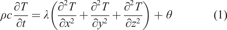
To solve this differential equation, initial conditions and boundary conditions need to be determined. At the thermal boundary, the heat flux is expressed as:

λ \frac{\partial T}{\partial n} = h (T_{a} - T_{v}) + q

(2)

where n is the normal to the surface, h is the convection coefficient, T_a is the ambient air temperature, T_v is the structural surface temperature, and q is the boundary heat flux.

For a bridge surface, the boundary heat flux q is the difference between emitted structural irradiation Gv and absorbed surrounding radiation I, which is expressed as follows:

q = I - G_{v}

(3)

The emitting structural radiation is estimated by:

G_{v} = C_{s} ε_{v} {T_{v}}^{4}

(4)

where C_s is the Stefan–Boltzmann constant, and ε_v is the emissivity coefficient of the structural surface.

The absorbed surrounding radiation is calculated as:

I = α I_{0}

(5)

where α is the absorptivity coefficient of the surface material and I₀ is the total radiation imposed on the surface, which includes direct, diffuse, and reflected solar radiation from the sun as well as atmospheric and ground radiation from the environment. During sunny weather, the radiation can be calculated based on theoretical equations.

The direct solar radiation I_s on a structural surface can be expressed by:

I_{s} = I_{s 0} \cos θ

(6)

I_{s 0} = 0 . 9^{t_{u} k_{a} m} I_{SC}

(7)

where I_s0 is the direct solar radiation on a horizontal plane, θ is the solar incidence angle to the structural surface, I_SC is the solar constant, t_u is the turbidity factor denoting the attenuation of radiation in different atmospheric conditions, k_a is the ratio of atmospheric pressure to pressure at sea level, and m is the air mass factor which equals 1/sinψ with ψ being the solar altitude angle.

The diffuse solar radiation I_i on a structural surface can be estimated using the Berlage formula (Berlage, 1959):

I_{i} = 0.5 (1 + \cos β) I_{i 0}

(8)

I_{i 0} = 0.5 I_{SC} \sin ψ \frac{1 - P^{m}}{1 - 1.4 \ln P}

(9)

P = 0 . 9^{t_{u} k_{a}}

(10)

where I_i0 is the diffuse solar radiation on a horizontal plane, P is the composite atmospheric transparency coefficient, and β denotes the tilt angle between the structural surface and horizontal plane.

The reflected solar radiation I_r on a structural surface can be calculated as:

I_{r} = 0.5 r_{e} (1 - \cos β) (I_{s 0} + I_{i 0})

(11)

where r_e is the reflection coefficient.

The atmospheric radiation is expressed as:

G_{a} = 0.5 ε_{a} C_{s} {(T_{k} + T_{a})}^{4} (1 - \cos β)

(12)

where ε_a is the atmospheric radiation coefficient, and T_k equals 273.15 K which is used for the conversion of degrees Celsius to absolute temperature.

The ground radiation G_g is calculated as:

G_{g} = 0.5 ε_{g} C_{s} {(T_{k} + T_{a})}^{4} (1 + \cos β)

(13)

where ε_g is the surface ground radiation coefficient.

The theoretical framework presented precedingly are primarily applicable to clear sky and cloudless conditions. However, under cloudy, rainy, or snowy weather scenarios, the actual solar radiation reaching the structure is significantly reduced due to cloud cover attenuation. This necessitates corresponding adjustment of the solar radiation intensity to accurately approximate the actual thermal boundary conditions.

Cloudy weather

Cloud conditions represent one of the most significant meteorological factors affecting solar radiation intensity. The attenuation of incoming solar radiation varies considerably depending on cloud characteristics. To quantitatively assess these effects, two key parameters are employed: illuminance and cloud cover. To obtain these parameters, a comprehensive environmental monitoring system is implemented in this study to collect continuous, long-term meteorological data. Integrating theoretical analysis and empirical data processing, we will develop three models: (1) an illuminance-based direct solar radiation correction model, (2) a cloud cover-based direct solar radiation correction model, and (3) a cloud cover-based diffuse solar radiation correction model. These models collectively provide a robust framework for comprehensive solar radiation quantification under diverse climatic conditions.

Design and implementation of the monitoring system

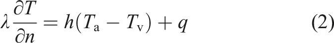
A compact automated meteorological monitoring station was strategically installed at an unobstructed open site in the Tianhe Campus of South China University of Technology to conduct continuous long-term environmental observations. The station systematically records multiple atmospheric parameters, including ambient temperature, relative humidity, wind direction and speed, various solar radiation components (direct, diffuse, and global), precipitation, and dew point temperature. A 170° wide-angle camera was installed at the monitoring site to capture sky images at one-minute intervals. These images were subsequently processed to extract grayscale values, which provide a quantitative metric for assessing the illuminance. The complete configuration of the monitoring system is illustrated in Figure 1.

Figure 1.

The layout of the monitoring system at the campus.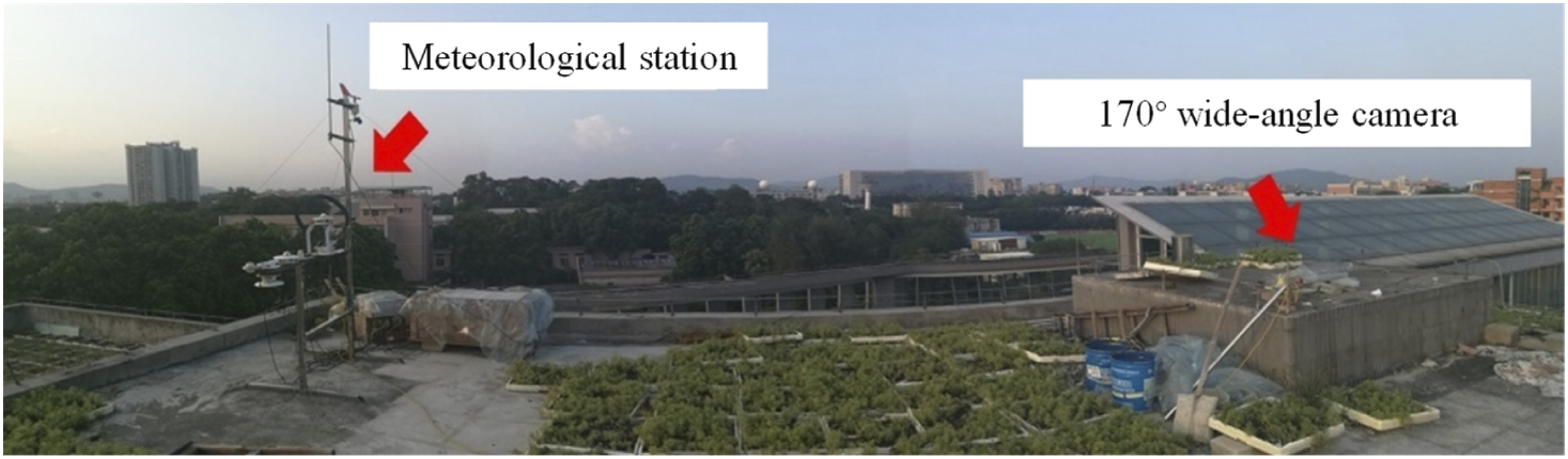

Illuminance-based direct solar radiation correction model

Continuous meteorological measurements were systematically acquired from June through August 2017 at the experimental site, resulting in 3455 valid datasets for solar radiation-illuminance correlation analysis. To facilitate robust comparative evaluation and parameter weighting across different measurements, the direct solar radiation correction coefficient is introduced, which is calculated as the ratio between the measured and theoretical direct solar radiation. Besides, the illuminance data are standardized as follows:

X = \frac{X_{0} - μ}{σ}

(14)

where X represents standardized illuminance data, X₀ denotes raw illuminance data with the unit of lux, and μ and σ are the mean and standard deviation of all samples, respectively.

The relationship between the direct solar radiation correction coefficient (Y_s) and measured standardized illuminance (X) at the monitoring site is illustrated in Figure 2. The results demonstrate a positive linear correlation between the correction coefficient and standardized illuminance, with a correlation coefficient of 0.837. Using the least-squares fitting method, the regression coefficients and confidence intervals were determined. The fitted regression line is also presented in the figure.

Figure 2.

Relation between direct solar radiation correction coefficient and illuminance.

The corresponding linear regression model is expressed as:

Y_{s} = 0.315 X + 0.149

(15)

Cloud cover-based direct and diffuse solar radiation correction models

Due to the practical challenges in measuring the localized cloud cover at the experimental site, this investigation uses cloud cover data from the Guangzhou Baiyun International Airport’s weather monitoring station, which is located approximately 20 km from the experimental site. The selected dataset comprises continuous recordings from June through August 2017, providing 136 valid cloud cover measurements for comprehensive correlation analysis.

When the cloud cover is 0%, the solar radiation correction coefficient is taken as 1. For cloud cover below 50%, the sky is classified as being under thin cloud conditions, where the correlation between cloud cover and actual solar radiation is weak. In contrast, when cloud cover exceeds 50%, obvious associations between cloud cover and both radiation correction coefficients are observed. The relationships between the cloud cover (C ≥0.5) and the direct (Y_s) and diffuse (Y_i) solar radiation correction coefficients are shown in Figure 3. Statistical analysis reveals notable linear relationships, with the correlation coefficients of 0.668 and 0.739 for Y_s and Y_i, respectively. The fitted regression line is also plotted in the figure.

Figure 3.

Relation between correction coefficients of solar radiations and cloud cover.

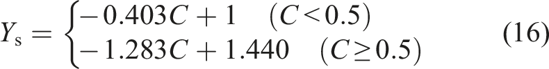
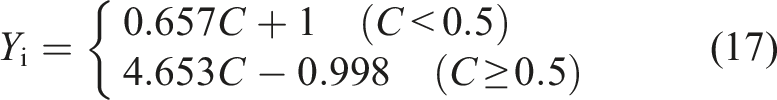
The corresponding linear regression models are expressed as two-stage piecewise linear functions. For cloud cover exceeding 50%, the relationships are derived from regression analysis, whereas for cloud cover below 50%, the values are determined by endpoint interpolation. The final cloud cover-based correction models for direct (Y_s) and diffuse (Y_i) solar radiation are expressed as follows:

Y_{s} = {\begin{cases} - 0.403 C + 1 (C < 0.5) \\ - 1.283 C + 1.440 (C \geq 0.5) \end{cases}

(16)

Y_{i} = {\begin{cases} 0.657 C + 1 (C < 0.5) \\ 4.653 C - 0.998 (C \geq 0.5) \end{cases}

(17)

Rainy and snowy weathers

In the rainy weather, besides solar radiation attenuation, structural surfaces require different thermal analyses according to the exposure conditions. In the rainy weather, the effective heat-transfer coefficient of the rain-exposed surfaces is determined as 12.7 W/(m²·K), with the rainwater temperature being the ambient air temperature. On other surfaces, thermal boundary conditions are consistent with those of the cloudy scenario. Additionally, the ground surface reflection coefficient needs to decrease correspondingly to account for the wetting effect.

In the snow weather, pure solid-solid conductive heat transfer is applied at the snow-structure interface, neglecting convective heat exchange. The snow temperature is conservatively maintained at 0°C. On other surfaces, thermal boundary conditions are consistent with those in cloudy weather. Meanwhile, the ground surface reflection coefficient should increase accordingly to account for the snow accumulation effect.

Computational framework under all-weather conditions

This study employs MATLAB as the central computational platform for configuring geographical environment parameters and analytical options. The weather condition is first autonomously classified as snowy, rainy, cloudy, or sunny scenarios according to meteorological monitoring data, including ambient temperature and precipitation. It should be noted that the sunny condition is categorized under the same scenario as the cloudy condition but with a specified solar radiation correction coefficient of 1. Then, the thermal boundary conditions are refined correspondingly by modifying solar radiation correction coefficients, specifying heat-transfer coefficients, or adjusting ground reflection coefficients. These parameters are subsequently exported to ANSYS for finite element analysis to calculate the structural temperature.

The proposed method achieves significant improvements in computational efficiency and accuracy by centralizing all parameter configurations within MATLAB, thereby enabling real-time, continuous high-performance analysis of bridge temperature distribution. The integrated computational framework is schematically illustrated in Figure 4.

Figure 4.

Computational framework for temperature calculation under all-weather conditions.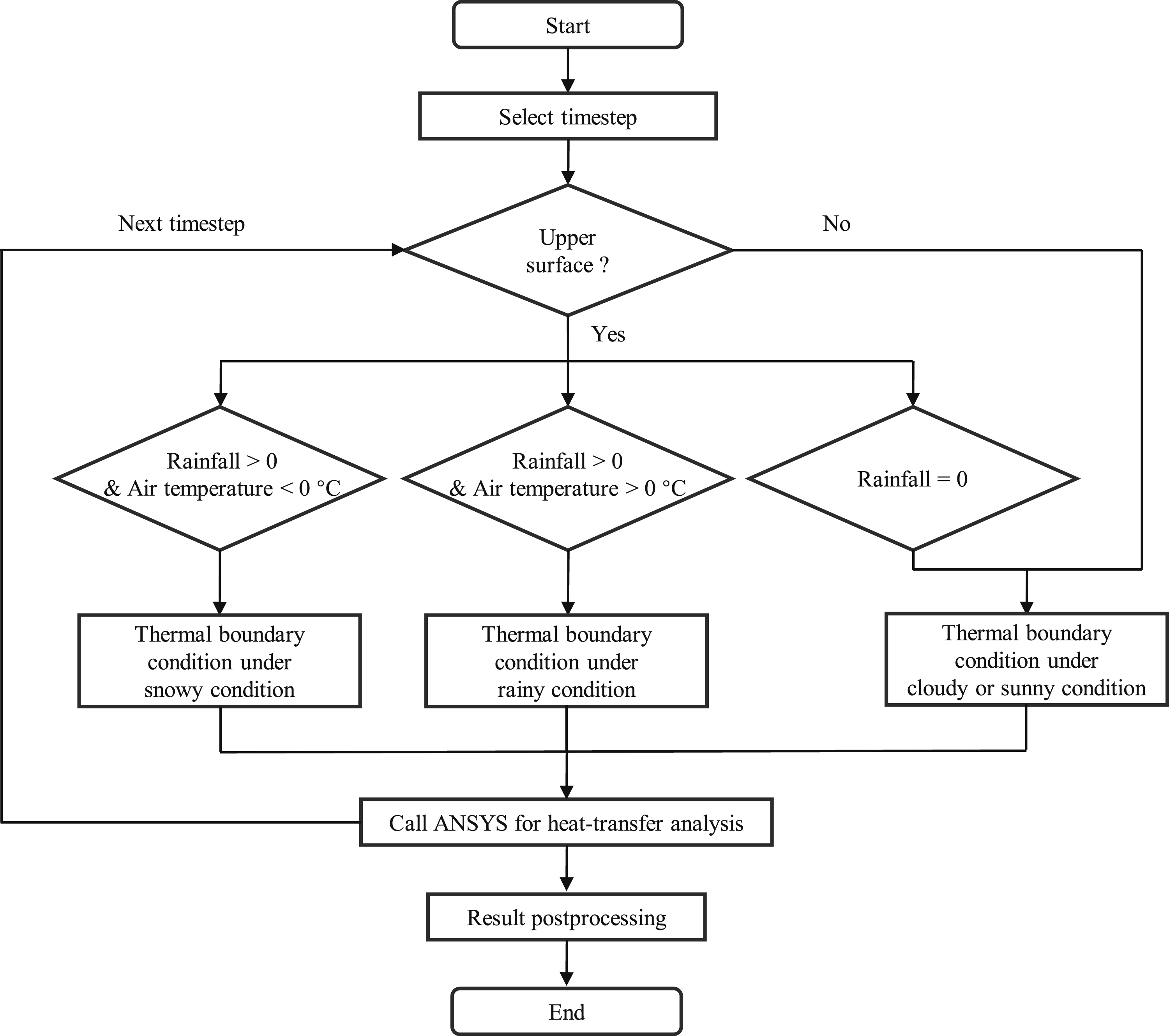

Case studies

To validate the effectiveness of the proposed methodology, three representative case studies are conducted on various girder sections with different materials and geometries: (1) an experimental RC slab, (2) a steel box girder suspension bridge, and (3) a concrete box girder continuous bridge.

Case study 1: An experimental RC slab

The RC slab specimen and test setup

The first case study involves an experimental investigation of an RC slab located at the same site as the meteorological monitoring station discussed in Section 2.1.2, with the test setup illustrated in Figure 5. An RC slab was placed on an insulated chamber and exposed to the ambient environment on the top. A small electric fan was placed within the chamber to facilitate air circulation. A predetermined quantity of ice was put into the chamber at 10:00 on the test day to induce a controlled temperature gradient in the vertical direction of the slab. Illuminance was measured using a 170° wide-angle camera, wind speeds with an anemometer, and ambient air temperature and relative humidity with a compact automatic weather station. T-type thermocouples were employed to monitor both the internal air temperature within the insulated chamber and the temperature distribution across the concrete slab. The dimensions of the slab and layout of thermocouples are shown in Figure 5(c). Four thermocouples were attached on the upper and lower surfaces at the same position, and three thermocouples were arranged at different depths to measure the temperature gradient.

Figure 5.

The RC slab specimen and test system.

Environmental conditions

November 9, 2017, characterized by relatively high solar radiation, low wind speed, and intermittent cloud cover, was selected for the heat-transfer analysis. Figure 6 presents the diurnal variations in temperature, illuminance, and wind speed on the day. In Figure 6(a), the temperature within the box exhibited a sharp decrease at 10:00 following the introduction of ice, which was intended to induce a prescribed temperature gradient between the upper and lower surfaces of the RC slab. By 12:00, the temperature within the chamber reached a minimum value of 14°C. Subsequently, as the ice melted, the temperature gradually increased, eventually approaching the ambient temperature by evening. Figure 6(b) depicts significant fluctuations in illuminance throughout the day, which were attributed to the dynamic cloud cover conditions. Figure 6(c) shows that the maximum wind speed recorded on that day did not exceed 3 m/s, indicating relatively low wind conditions.

Figure 6.

The environmental conditions on November 9, 2017.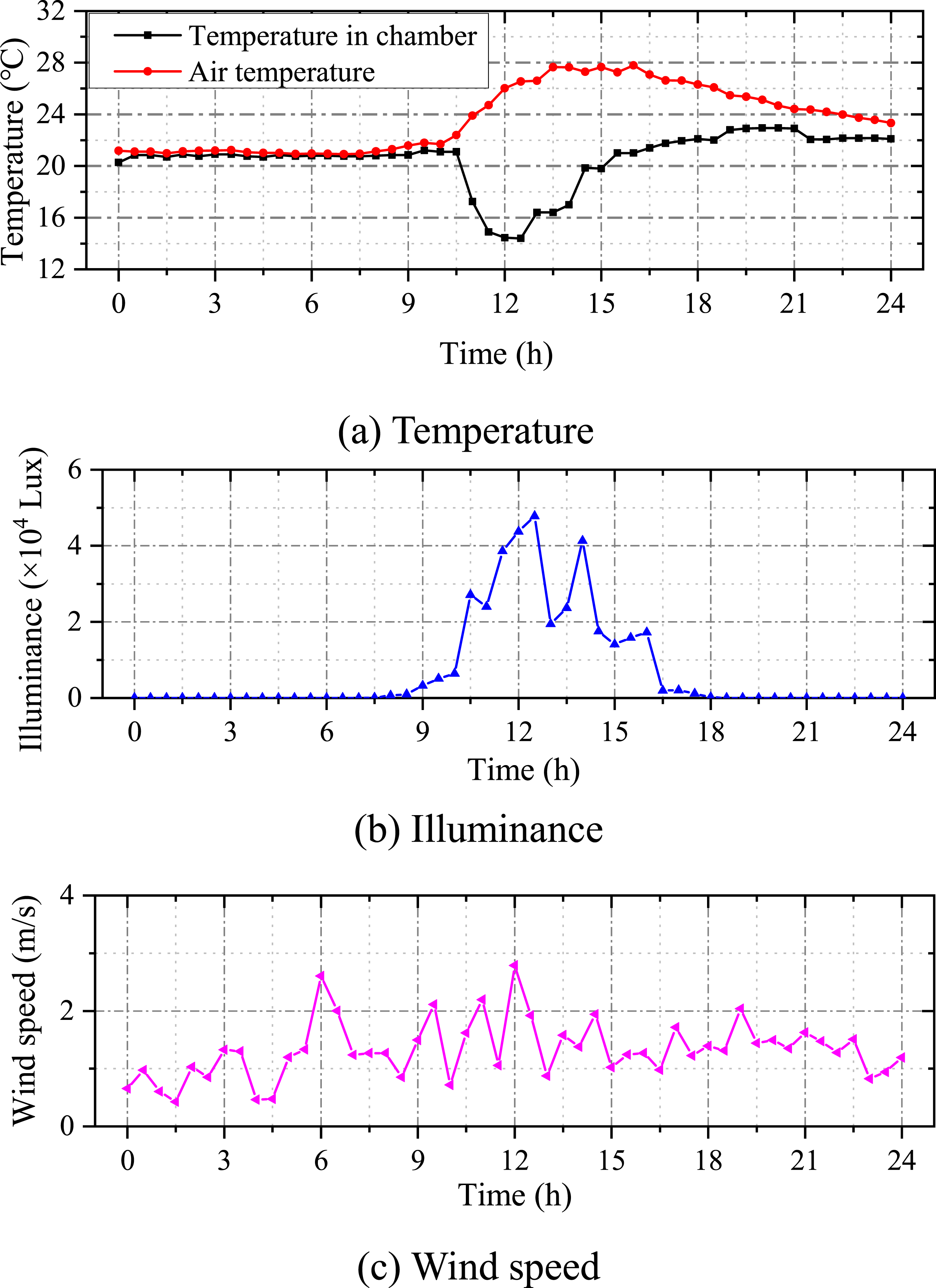

FEM of the RC slab

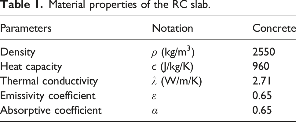
The FEM of the RC slab is established using SOLID70 elements in ANSYS (ANSYS 16.1), as shown in Figure 7. The material properties used in the heat-transfer analysis are listed in Table 1.

Figure 7.

FEM of the RC slab.

Table 1.

Material properties of the RC slab.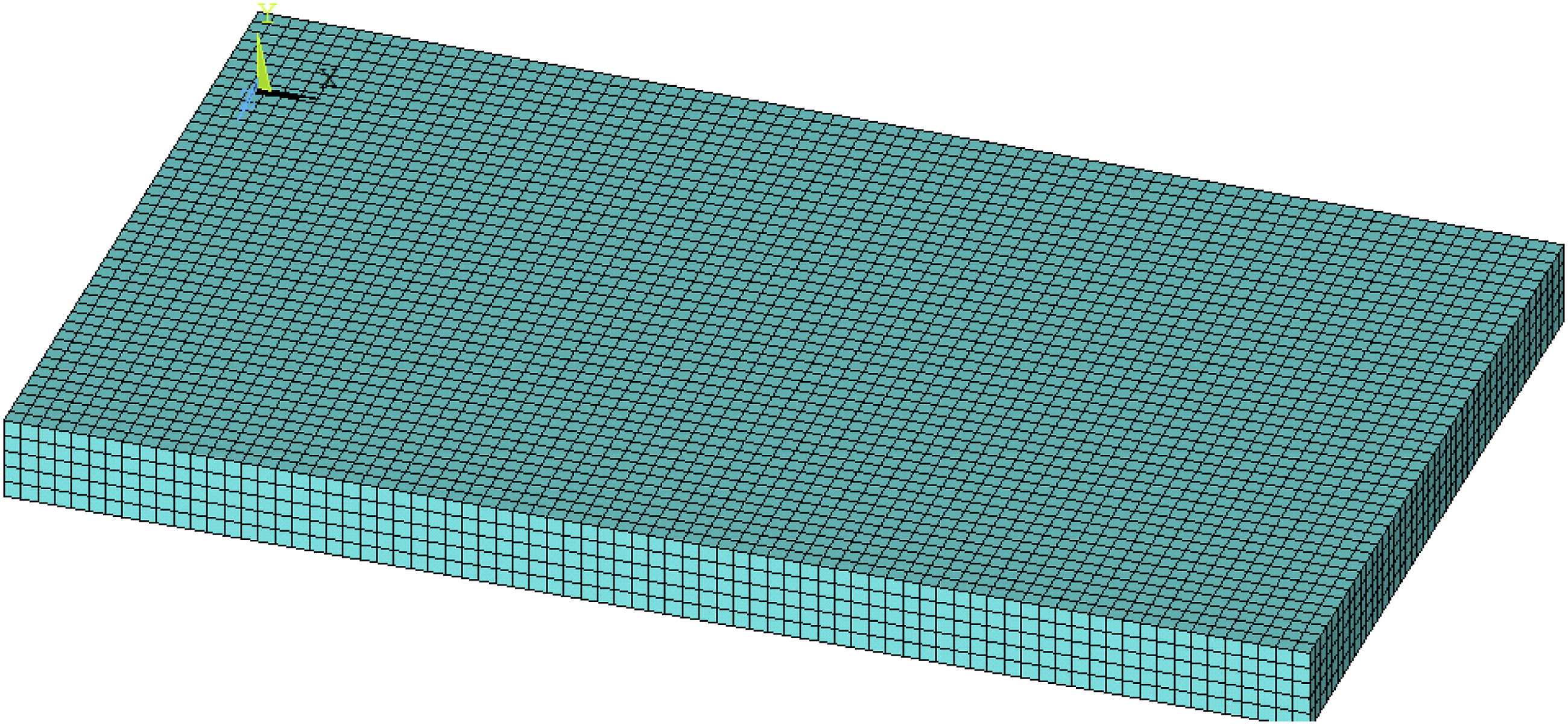

Parameters	Notation	Concrete
Density	ρ (kg/m³)	2550
Heat capacity	c (J/kg/K)	960
Thermal conductivity	λ (W/m/K)	2.71
Emissivity coefficient	ε	0.65
Absorptive coefficient	α	0.65

Temperature field of the RC slab

According to the environmental conditions, including the adjusted solar radiation, the thermal boundary conditions are calculated and applied to the FEM for the transient heat-transfer analysis. To establish a non-uniform initial equilibrium, a pre-analysis was conducted for the day preceding November 9, 2017 to mitigate the adverse effects of uncertain original conditions. In this pre-analysis, the air temperature was assigned as the initial temperature of the structure.

After the heat-transfer analysis, the temperature variations of the RC slab on November 9, 2017 are obtained and compared with the corresponding measurements in Figure 8. In the early morning, the air temperature remained lower than the temperature inside the chamber, resulting in the bottom of the concrete slab being slightly warmer than the top. As the sun rose, the temperature of the top surface increased rapidly, exceeding that of the bottom surface. At noon, the temperature difference between the top and bottom of the concrete slabs reached 6°C, which was accentuated by the strategic placement of ice within the chamber intended to enforce a controlled thermal gradient. During nighttime, diminished solar radiation and melted ice caused the temperature of the interior of the chamber to exceed the exterior. This induced heat transfer from the bottom of the slab to the top, resulting in a negative temperature differential. The numerical simulation effectively captures the thermal behavior of concrete slabs under cloudy conditions. The good agreement between the simulated and measured temperatures demonstrates the effectiveness of the heat-transfer analysis method proposed in this study.

Figure 8.

Measured and simulated temperatures of the RC slab on November 9, 2017.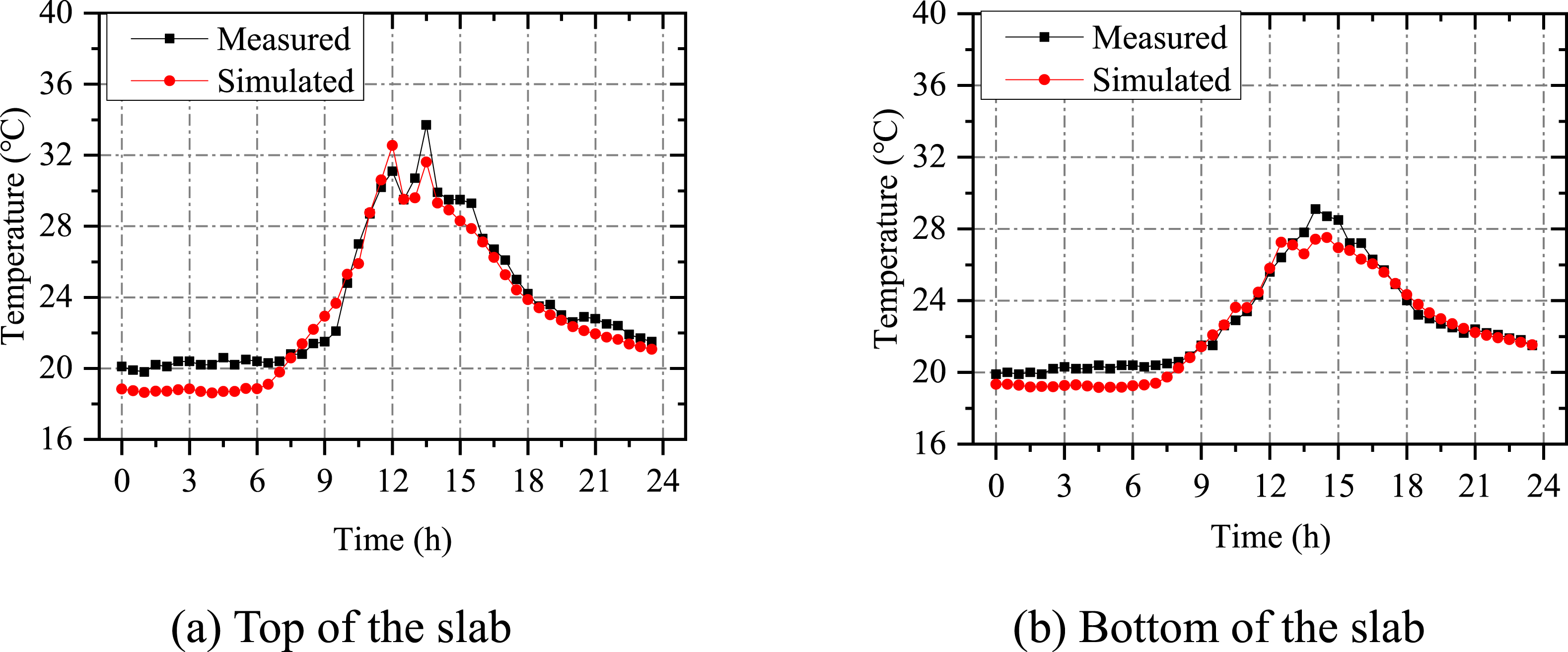

Case study 2: A steel box girder suspension bridge

The steel box girder suspension bridge and its temperature measurements

The second case study examines the Humber Bridge, a steel box-girder suspension bridge located in the UK. With a total length of 2220 m, the structure comprises a 280-m northern side span, a 1410-m central span, and a 530-m southern side span, as depicted in Figure 9. The main girder features a stiffened steel box configuration with a width of 22 m and a depth of 4.5 m, surfaced with a 41-mm-thick asphalt layer.

Figure 9.

The steel box girder suspension bridge.

Six thermometers were positioned at the mid-span girder section, as depicted in Figure 10. The measurement points are identified as follows: T_s—surface temperature of the asphalt pavement, T_g—temperature at the interface between the steel box and the asphalt pavement, T_t—temperature of the top plate of the steel box, T_b—temperature of the bottom plate of the steel box, T_e—temperature of the upper web on the east side, and T_w—temperature of the upper web on the west side.

Figure 10.

Layout of temperature sensors on the Humber Bridge.

Environmental conditions

A representative rainy day, April 17, 2012, characterized by relatively low solar radiation, persistent cloud cover, and intermittent rainfalls, is selected for analysis. Meteorological data, including ambient temperature, precipitation duration, wind speed, and cloud cover, are acquired from Humberside Airport’s monitoring station through the National Oceanic and Atmospheric Administration database (NOAA, 2025) and shown in Figure 11. As depicted in Figure 11(a), the ambient temperature experienced a pronounced decrease starting at 3:30 due to rainfall, ultimately reaching the minimum of 3°C at 5:30. Subsequent to precipitation cessation at 09:30 and increasing solar radiation, the temperature started to increase. The ambient temperature experienced another two slight decreases at 11:30 and 15:00 due to intermittent showers. It should be noted that the meteorological station’s recorded precipitation events may differ from the actual conditions at the bridge site.

Figure 11.

The environmental conditions on April 17, 2012.

FEM of the steel box girder section

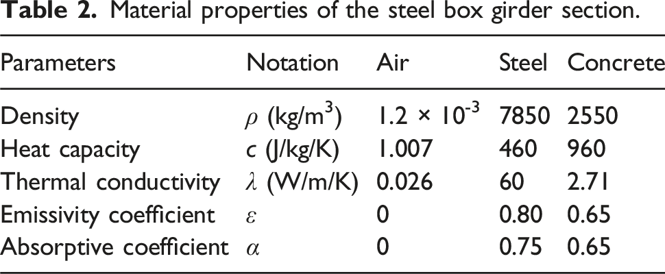
The FEM of the steel box girder section, consisting of 38,620 elements, is shown in Figure 12. The model employs PLANE55 elements to simulate the steel stiffened plate, asphalt layer, and internal air (ANSYS 16.1). The material properties of the steel box girder section used in the heat-transfer analysis are presented in Table 2.

Figure 12.

FEM of the steel box girder section.

Table 2.

Material properties of the steel box girder section.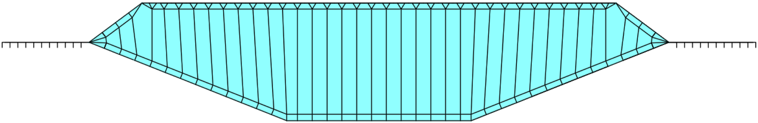

Parameters	Notation	Air	Steel	Concrete
Density	ρ (kg/m³)	1.2 × 10^-3	7850	2550
Heat capacity	c (J/kg/K)	1.007	460	960
Thermal conductivity	λ (W/m/K)	0.026	60	2.71
Emissivity coefficient	ε	0	0.80	0.65
Absorptive coefficient	α	0	0.75	0.65

Temperature field of the steel box girder section

The temperature variations of the steel box girder on April 17, 2012 are calculated by integrating the cloud cover-based solar radiation correction models into the heat-transfer analysis. The simulated temperature distributions are subsequently compared with field measurements in Figure 13. Between 4:00 and 10:00, the temperature of the box girder remained relatively low due to the rainfall. Once the rain ceased, the temperature of the box girder increased rapidly due to solar radiation, with the temperature of the top asphalt reaching 21°C. Although the bottom plate was not exposed to direct solar radiation, it experienced gradual temperature increases due to rising ambient temperatures and indirect radiative heat transfer. The simulated temperatures exhibit a good alignment with the measured results, with discrepancies mainly attributed to the environmental differences between the meteorological station and the bridge site.

Figure 13.

Measured and simulated temperatures of the steel box girder section on April 17, 2012.

Case study 3: A concrete box girder continuous bridge

The concrete box girder continuous bridge and its temperature measurements

The third case study is a prestressed concrete box girder continuous bridge in Tangshan, China (Zhang, 2017). The studied bridge has a total length of 1015.3 m, as illustrated in Figure 14. The deck is paved with an 8-cm-thick layer of reinforced concrete and a 10-cm-thick layer of asphalt.

Figure 14.

The prestressed continuous box girder bridge.

Figure 15 illustrates the layout of six thermocouples installed on the prestressed continuous box girder bridge to measure its temperature distribution. The measurement points are identified as follows: T₁—temperature of the top surface of the top plate, T₂—temperature of the bottom surface of the top plate, B₁—temperature of the top surface of the bottom plate, B₂—temperature of the bottom surface of the bottom plate, W₁—temperature of the east web, and W₂—temperature of the west web.

Figure 15.

Layout of temperature sensors on the prestressed continuous box girder bridge.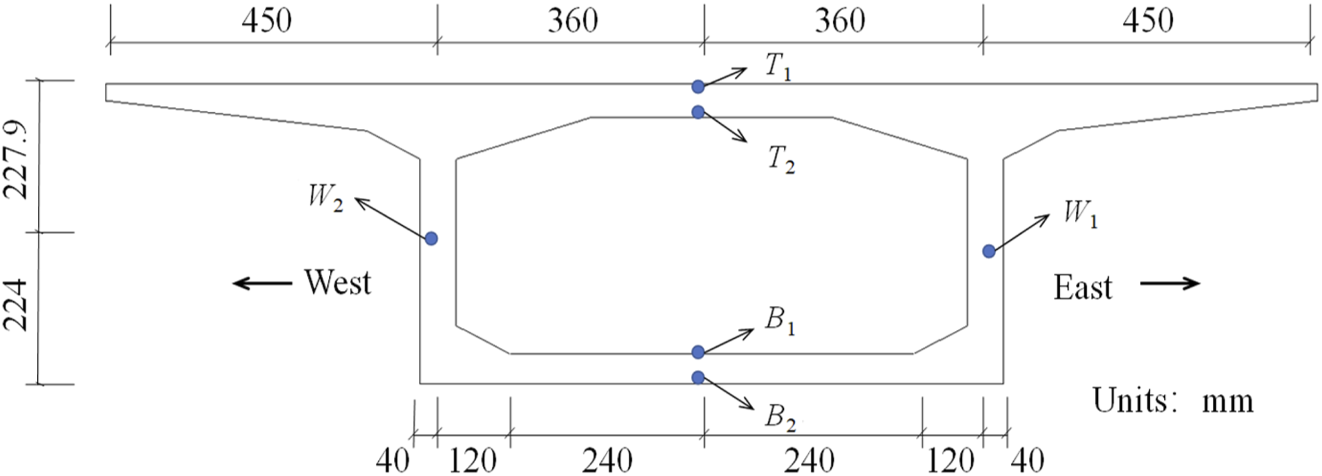

Environmental conditions

August 7, 2016, a cloudy day characterized by relatively low solar radiation, is selected for analysis. Figure 16 shows the air temperature, wind speed, and cloud cover measurements at the Tangshan Sannuhe Airport obtained from the National Oceanic and Atmospheric Administration website (NOAA, 2025).

Figure 16.

The environmental conditions on August 7, 2016.

FEM of the concrete box girder section

The FEM of the steel box girder section, consisting of 2418 elements, is shown in Figure 17. The model adopts PLANE55 elements to simulate the concrete box and the internal air (ANSYS 16.1). The material properties are the same as those listed in Table 2.

Figure 17.

FEM of the concrete box girder section.

Temperature field of the concrete box girder section

By integrating the cloud cover-based solar radiation correction models into the heat-transfer analysis, the temperature variations of the concrete box girder under cloudy weather on August 7, 2016 are calculated. Since Zhang (2017) only contains measurement data from 6:00 to 19:00 on the day, the results during this period are compared in Figure 18. The simulated and measured temperatures have a good agreement. The top plate experienced a significant temperature increase of 10°C due to direct solar radiation during the day and reached a maximum of 38°C at 14:00. The bottom surface of the bottom plate was subjected to a minor temperature increase of 4°C on account of the reflected solar radiation. The inner surfaces of the box girder show a relatively lower temperature variation. Meanwhile, the temperatures of the webs remained almost unchanged, which is attributed to the insufficient diffuse solar radiation under the cloudy weather.

Figure 18.

Measured and simulated temperatures of the concrete box girder section on August 7, 2016.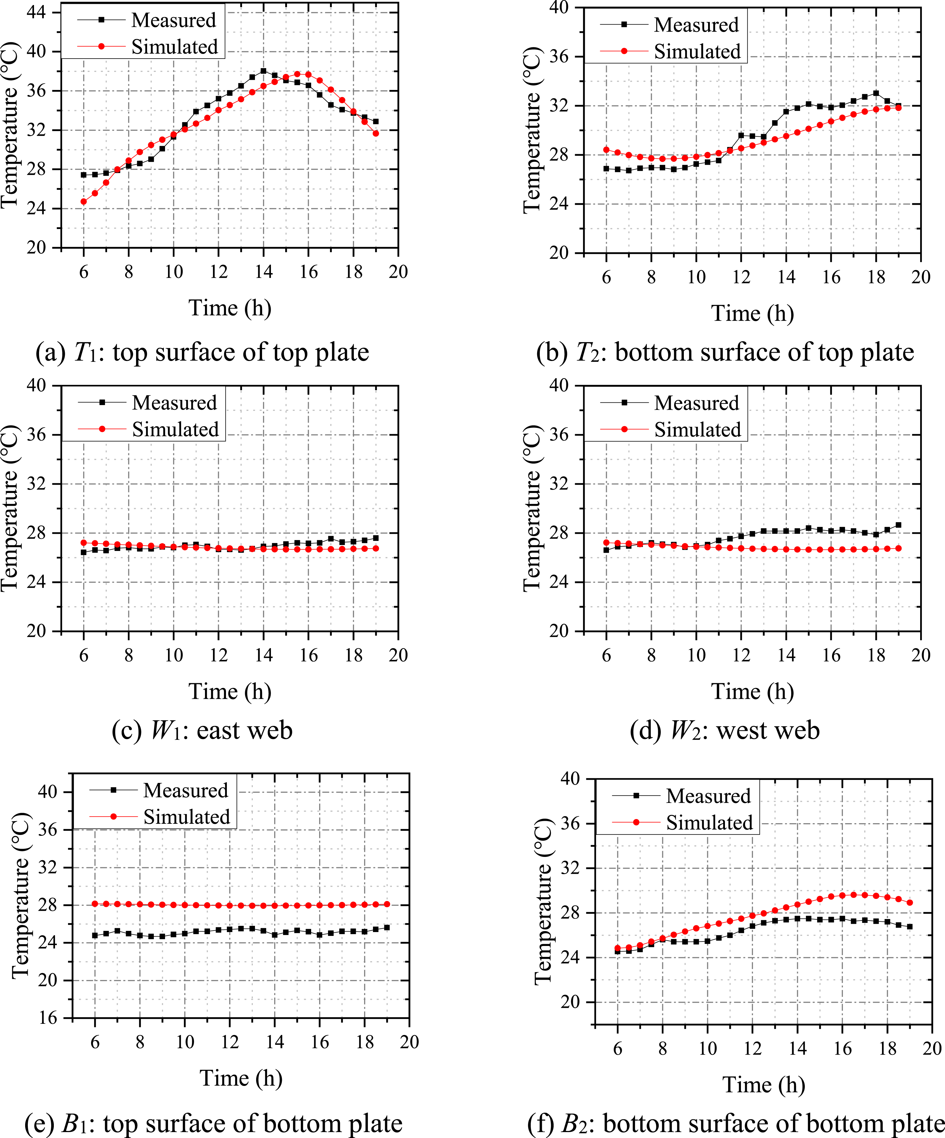

Conclusions

A numerical method for calculating bridge temperature under different weather conditions has been developed by integrating illuminance and cloud cover parameters into the heat-transfer analysis. According to real-time data of illuminance and cloud cover, the shielding effect of clouds on solar radiation is quantified using solar radiation correction models. The thermal boundary conditions are then determined with other meteorological parameters, including air temperature and wind speed. A computational framework has been developed for automatic weather scenario classification, boundary condition determination, and heat-transfer analysis. After the refined heat-transfer analysis, the temperature distribution of bridge structures under different weather conditions can be accurately obtained. The proposed method has been validated through three case studies, including an experimental RC slab, a steel box girder suspension bridge and a concrete box girder continuous bridge with a field monitoring system. The following conclusions can be drawn:

(1) The three proposed correction models—namely, the illuminance-based direct solar radiation correction model, the cloud cover-based direct solar radiation correction model, and the cloud cover-based diffuse solar radiation correction model—effectively enhance the heat-transfer analysis accuracy under various weather conditions.

(2) In the experimental case study on the RC slab under cloudy weather, illumination data are used to adjust the theoretical solar radiation. The good agreement between the simulated temperatures and field measurements verifies the effectiveness of the proposed illuminance-based direct solar radiation correction model in heat-transfer analysis across diverse weather conditions.

(3) In the two real bridges with SHM systems—a steel box girder suspension bridge and a concrete box girder continuous bridge—cloud cover data are employed to adjust the theoretical solar radiation. The close alignment between simulated and measured temperatures further validates the effectiveness of the proposed cloud cover-based direct and diffuse solar radiation correction models in heat-transfer analysis under varying weather conditions.

Footnotes

ORCID iDs

Linren Zhou

Shiping Huang

Yushi Shan

Funding

The authors disclosed receipt of the following financial support for the research, authorship, and/or publication of this article: This research was supported by the National Natural Science Foundation of China (Project No. 52078220), the International Science & Technology Cooperation Program of Guangdong Province (Project No. 2023A0505050155), and PolyU Internal Project (Project No. CDKL). Sincere gratitude also goes to Professor Brownjohn and his team for their invaluable support in providing data for this study.

Declaration of conflicting interests

The authors declared no potential conflicts of interest with respect to the research, authorship, and/or publication of this article.

References

Abid

Xue

Liu

, et al. (2022) Temperatures and gradients in concrete bridges: experimental, finite element analysis and design. Structures 37: 960–976.

Al-Khateeb

Shenton

Chajes

(2018) Computing continuous load rating factors for bridges using structural health monitoring data. Journal of Civil Structural Health Monitoring 8: 721–735.

ANSYS 16.1. Southpointe, PA, USA. [Computer Software].

Berlage

(1959) The basic scheme of any planetary or satellite system corrected and reanalyzed. Proceedings of the Koninklijke Nederlandse Akademie, B 62: 63–83.

Chang

Flatau

Liu

(2003) Health monitoring of civil infrastructure. Structural Health Monitoring 2(3): 257–267.

Elbadry

Ghali

(1983) Temperature variations in concrete bridges. Journal of Structural Engineering 109(10): 2355–2374.

Emerson

(1973) The calculation of the distribution of temperature in bridges. In: TRRL Rep. No. LR561. Crowtowne, U.K: Department of the Environment.

Liu

Lao

(2025) Assessing temperature-induced deflections in cable-stayed bridges during construction: an elastic foundation beam model approach. Journal of Bridge Engineering 30(1): 04024104.

Fujino

Murata

Okano

, et al. (2000) Monitoring system of the Akashi Kaikyo Bridge and displacement measurement using GPS. Nondestructive Evaluation of Highways, Utilities, and Pipelines IV(3995): 229–236.

10.

Gilliland

Dilger

(1997) Monitoring concrete temperature during construction of the confederation bridge. Canadian Journal of Civil Engineering 24(6): 941–950.

11.

Gong

Sun

Chen

(2024) Analysis of coupled thermo-mechanical response and damage behaviour of curved ramp bridge deck pavement using a 3D multiscale method. Road Materials and Pavement Design 25(11): 2335–2357.

12.

Hajializadeh

(2023) Deep learning-based indirect bridge damage identification system. Structural Health Monitoring 22(2): 897–912.

13.

Jing

Shan

Zhang

, et al.. (2024) Typhoon-and temperature-induced responses of a cable-stayed bridge. Advances in Structural Engineering 27(16): 2773–2789.

14.

Lei

Siringoringo

Sun

, et al. (2023) Displacement response estimation of a cable-stayed bridge subjected to various loading conditions with one-dimensional residual convolutional autoencoder method. Structural Health Monitoring 22(3): 1790–1806.

15.

Zhang

, et al. (2022) Automatic uncoupling of massive dynamic strains induced by vehicle-and temperature-loads for monitoring of operating bridges. Mechanical Systems and Signal Processing 166: 108332.

16.

Chen

Zhou

, et al. (2023) Thermal behaviors of bridges—A literature review. Advances in Structural Engineering 26(6): 985–1010.

17.

Lin

Briseghella

Xue

, et al. (2020) Temperature monitoring and response of deck-extension side-by-side box girder bridges. Journal of Performance of Constructed Facilities 34(2): 04019122.

18.

Manconi

Shahmirzaloo

Moonen

SPGF

(2025) Thermo-mechanical analysis of extreme thermal loads on a flax fiber composite sandwich footbridge. Composites Part B: Engineering 292: 112084.

19.

Meng

Sun

Dang

, et al. (2025) Deep learning-based minute-scale digital prediction model for temperature induced deflection of a multi-tower double-layer steel truss bridge. Advances in Structural Engineering 28(1): 4–22.

20.

Naruoka

Hirai

Yamaguti

(1957) The measurement of the temperature of the interior of the reinforced concrete slab of the Shigita Bridge and presumption of thermal stresses. In: Symposium on the Stress Measurements for Bridge and Structure, pp. 106–115.

21.

Niu

Guo

(2023) Application of a thermodynamic model in durability analysis of bridge structures under climatic variability. International Journal of Heat & Technology 41(4).

22.

NOAA (2025) “National Oceanic and Atmospheric Administration.”. Available from. https://www.noaa.gov/

23.

(2005) The state-of-the-art and practice of structural health monitoring for civil infrastructures in the mainland of China. Proceedings of the Second International Conference on Structural Health Monitoring and Intelligent Infrastructure. Shenzhen, China, 1, 69–93.

24.

Shahawy

Arockiasamy

(1996) Field instrumentation to study the time-dependent behavior in sunshine skyway bridge. Journal of Bridge Engineering 1(2): 76–86.

25.

Shan

Xia

, et al. (2023) Temperature behavior of cable-stayed bridges. Part I—global 3D temperature distribution by integrating heat-transfer analysis and field monitoring data. Advances in Structural Engineering 26(9): 1579–1599.

26.

Sun

(2018) Jiangyin bridge: an example of integrating structural health monitoring with bridge maintenance. Structural Engineering International 28(3): 353–356.

27.

Tayşi

Abid

(2015) Temperature distributions and variations in concrete box-girder bridges: experimental and finite element parametric studies. Advances in Structural Engineering 18(4): 469–486.

28.

Wang

Zhan

Zhao

(2016) Analysis of thermal behavior on concrete box-girder arch bridges under convection and solar radiation. Advances in Structural Engineering 19(7): 1043–1059.

29.

Wang

Zhang

Lei

, et al. (2021) All-weather thermal simulation methods for concrete maglev bridge based on structural and meteorological monitoring data. Sensors 21(17): 5789.

30.

Wang

Zhang

Wang

, et al. (2024) Investigation of temperature effects on wide steel box girder of suspension bridge based on long-term monitoring data. Scientific Reports 14(1): 9691.

31.

Xia

Chen

Zhou

, et al. (2013) Field monitoring and numerical analysis of Tsing Ma suspension bridge temperature behavior. Structural Control and Health Monitoring 20(4): 560–575.

32.

Xia

Liu

Zhang

(2020b) Temperature analysis of a long-span suspension bridge based on a time-varying solar radiation model. Smart Structures and Systems. An International Journal 25(1): 23–35.

33.

Xia

, et al. (2022) Temperature behaviors of an arch bridge through integration of field monitoring and unified numerical simulation. Advances in Structural Engineering 25(16): 3492–3509.

34.

Xia

Wan

, et al. (2020a) Condition analysis of expansion joints of a long‐span suspension bridge through metamodel‐based model updating considering thermal effect. Structural Control and Health Monitoring 27(5): e2521.

35.

Xia

(2012) Structural Health Monitoring of Long-Span Suspension Bridges. CRC Press.

36.

Zhang

(2017) The Most Unfavorable Solar Temperature Field and Thermal Stress of long-span Concrete Box Girder. Southwest Jiaotong University.

37.

Zhou

Xia

Chen

, et al. (2020) Analytical solution to temperature-induced deformation of suspension bridges. Mechanical Systems and Signal Processing 139: 106568.

38.

Zhou

Zheng

Hao

, et al. (2023) A temperature effect prediction method for long-span bridges based on meteorological big data. Journal of Hunan University 15: 1–13.

39.

Zhou

Wang

Chen

(2024a) Bridge temperature prediction method based on long short-term memory neural networks and shared meteorological data. Advances in Structural Engineering 27(8): 1349–1360.

40.

Zhou

Wanyan

(2024b) Review on convective and radiation heat transfer between bridges and external environments. Advances in Structural Engineering 27(8): 1285–1302.

41.

Zhu

Meng

Shi

, et al. (2023) Long-term deformation analysis of prestressed concrete bridges under ambient thermal and vehicle loads. Structure and Infrastructure Engineering 19(11): 1656–1675.

42.

Zuk

(1965) Thermal behaviour of composite bridges-insulated and uninsulated. Highway Research Record 76(1): 231–253.