Axle-information-free identification of vehicle moving forces from bridge displacement using U-Net

Abstract

Traffic loads are the main source of live loads on bridge structures, and accurately identifying the dynamic axle load of vehicles is of great importance for Bridge Structural Health Monitoring (BSHM). Most of the past research established the relationship between moving forces and structures through analytical or finite element methods to estimate axle loads, which was proved to be ill-conditioned and inefficient. In this paper, a Moving Force Identification (MFI) method based on U-shaped Network (U-Net) is proposed, which does not require axle position information as a prior knowledge, but is completely based on monitoring data. Firstly, the dynamic response of the finite element model under traffic load is used to establish a data set. In this process, a large number of random traffic flows with different axle loads, axle spacings and vehicle speeds are generated to simulate the operation process of real bridges. Then, the deep learning model is trained with dynamic displacement data as input and dynamic axial load as output. The accuracy of the model is verified by numerical simulation and the robustness of the model is tested. Finally, the practicality of the proposed method is tested by the actual bridge experiment. The results of the actual bridge test show that the mean error of the axle force identification of the proposed method is 6.28 %, indicating that the proposed method has certain application prospects in practical engineering.

Keywords

moving force identification dynamic axle load identification U-Net deep learning bridge structural health monitoring

Introduction

As a critical component of road infrastructure, bridges play an essential role in transportation networks, and their safety depends on both structural performance and external loads. Among these, traffic loads constitute the primary live load during bridge operation. Accurate identification of vehicle–bridge interaction forces is therefore of great importance for bridge design, assessment, and maintenance.

Various methods have been developed to monitor traffic loads on bridges, which can be broadly classified into direct and indirect approaches. Direct measurement methods, commonly referred to as Weigh-in-Motion (WIM) systems (Richardson and Jones, 2014), employ sensors embedded in the road surface to measure tire-induced dynamic pressures, enabling the estimation of axle loads, axle counts, and vehicle speeds (Sujon and Dai, 2021). Although WIM systems can operate without interrupting traffic, they typically suffer from short service life and high installation and maintenance costs. Their installation often requires lane closures and may cause damage to the bridge deck (Yu et al., 2016). Moreover, since traffic loads vary in both time and space, WIM systems cannot directly capture the time-history distribution of vehicle loads acting on the entire bridge (Burnos and Gajda, 2016). Consequently, indirect measurement techniques, which are more cost-effective and less intrusive, have attracted increasing research attention.

Indirect measurement techniques, commonly referred to as Moving Force Identification (MFI), model traffic loads as moving forces acting on the bridge. By exploiting measured structural responses and the relationship between these responses and vehicle loads, MFI enables the back-calculation of axle loads and total vehicle weight, yielding the time history of the moving force. As an important research topic in Structural Health Monitoring (SHM), MFI has been extensively investigated over the past decades (Yi et al., 2017). Based on different calculation methods, MFI algorithms can be divided into analytical methods (Zuo et al., 2019) and finite element methods (Hao et al., 2019). Analytical methods require a mathematical model to obtain the dynamic response of the bridge and solve an optimization problem where the contact force is the variable of the objective function. This optimization minimizes the difference between the analytical response and the sensor measurements. Analytical methods include the time domain method (Law et al., 1997), time-frequency domain method (Yu and Chan, 2003), interpretation method (Chan et al., 1999), state-space method (Zhu et al., 2006), moment method (Yu et al., 2008), and influence line method (Jian et al., 2019; Wang et al., 2025).

Finite element methods, on the other hand, establish a finite element model of the bridge to derive the relationship between the moving force and a particular component. Since the MFI problem is a typical inverse problem, its solution is highly sensitive to noise, road roughness and initial conditions, and it may encounter significant errors when the moving forces are near the structural boundaries (Cao, 2025; Pan et al., 2017). To mitigate these issues, regularization methods are often incorporated into the MFI solution process (Jian et al., 2022). Common regularization methods include Tikhonov regularization (Zhu and Law, 2002), basis function expansion method (Qiao et al., 2015), sparse regularization method (Pan et al., 2018), Bayesian inference regularization (Feng et al., 2015), truncated singular value decomposition (Chen and Chan, 2017) and so on. For instance, Tang et al. (Tang et al., 2022) introduced a load identification method based on the transmissibility of power spectral density and adaptive multiplicative regularization. Their approach can localize random loads without prior knowledge of the excitation position and significantly reduces the iteration cost. Despite these advances, the iterative solution of dynamic equilibrium equations still imposes a considerable computational cost, making it difficult to achieve real-time performance. Moreover, most existing MFI methods require additional measurements, such as vehicle speed, axle spacing, and axle number, obtained from camera systems or auxiliary sensors (Jian et al., 2024; Wang and Li, 2025; Zhang et al., 2021), which further complicates practical implementation.

In recent years, advances in computational power and artificial intelligence have motivated the application of deep learning techniques to moving force identification. Owing to their strong nonlinear modeling capability, neural networks can learn the complex mapping between structural responses and vehicle loads, thereby avoiding the explicit solution of time-consuming inverse problems. (Kim et al., 2009) employed artificial neural networks to identify vehicle weight, speed, and axle information from strain measurements, demonstrating accuracy comparable to traditional influence-line methods on a cable-stayed bridge. (Chang et al., 2025) proposed a low-complexity real-time detection Transformer (LC-RTDETR) that improves vehicle localization accuracy under dynamic scenes while reducing computational cost. (Kawakatsu et al., 2019) used deep neural networks with a single strain sensor to estimate vehicle speed, trajectory, and wheel position, aided by temporary camera-based calibration. (Zeng et al., 2024) proposed a Moving Force Neural Identifier incorporating a dynamic moving force correction block to estimate dynamic axle loads without explicit vehicle speed or axle information. However, this approach considers only a limited set of predefined vehicle configurations, and its applicability to real bridge scenarios requires further validation.

In summary, although MFI techniques have achieved significant progress, they still face challenges such as sensitivity to noise, high computational cost, and reliance on additional information including vehicle speed, axle spacing, and axle count. Developing MFI methods that satisfy real-time requirements while relying solely on structural response data remains a major challenge. Deep learning–based MFI approaches offer the potential to implicitly extract axle-related information from monitoring data, thereby eliminating the need for dedicated axle detection equipment. However, existing studies are still at an early stage, with most investigations limited to numerical simulations or laboratory-scale experiments, and often focused on static or quasi-static axle load estimation. Consequently, there is a strong demand for efficient methods capable of accurately identifying dynamic axle loads. Motivated by these challenges, this study proposes a U-Net–based vehicle dynamic load identification method that fully exploits structural response data. The proposed approach enables accurate estimation of dynamic axle loads without requiring prior information such as axle count or axle spacing.

This paper is organized as follows: Section 2 introduces the framework of MFI and the simplified vehicle-bridge interaction system. Section 3 presents the results of numerical simulation verification and model robustness analysis. Section 4 evaluates the feasibility of the proposed method for engineering applications through vehicle testing on a real bridge. Finally, the conclusion is given in Section 5.

To assist readers unfamiliar with the notation used in moving force identification, the main variables and their corresponding units are summarized in Table 1.

Table 1.

Nomenclature of main variables used in the paper.

Symbol	Description	Unit
$t$	Time	s
$F_{l o a d} (t)$	Axle force time history acting on the bridge	kN
$F_{s t a t i c} (t)$	Static component of $F_{l o a d} (t)$	kN
$F_{d y n a m i c} (t)$	Dynamic component of $F_{l o a d} (t)$	kN
$A_{i}$	Amplitude of the i-th dynamic load component	-
$ω_{i}$	Angular frequency of the i-th dynamic load component	rad/s
$F_{w h i t e n o i s e} (t)$	Additive white noise term representing random fluctuations in $F_{l o a d} (t)$	kN
$W$	Total axle weight of the vehicle	t
$R$	Front axle weight ratio	-
$b_{x}$	Front and rear axle spacing	m
$b_{y}$	Left and right wheel spacing	m
$v$	Speed	km/h
RPE	Relative percentage error	%

Methodology

Figure 1 illustrates the proposed moving force identification framework. First, a finite element model of the bridge is established based on design documents and calibrated using field monitoring data. The updated model is then used to generate simulation datasets for training the U-Net. Finally, the trained network is applied to displacement measurements from the real bridge to identify the time-history of vehicle loads.

Figure 1.

Framework of the proposed MFI method.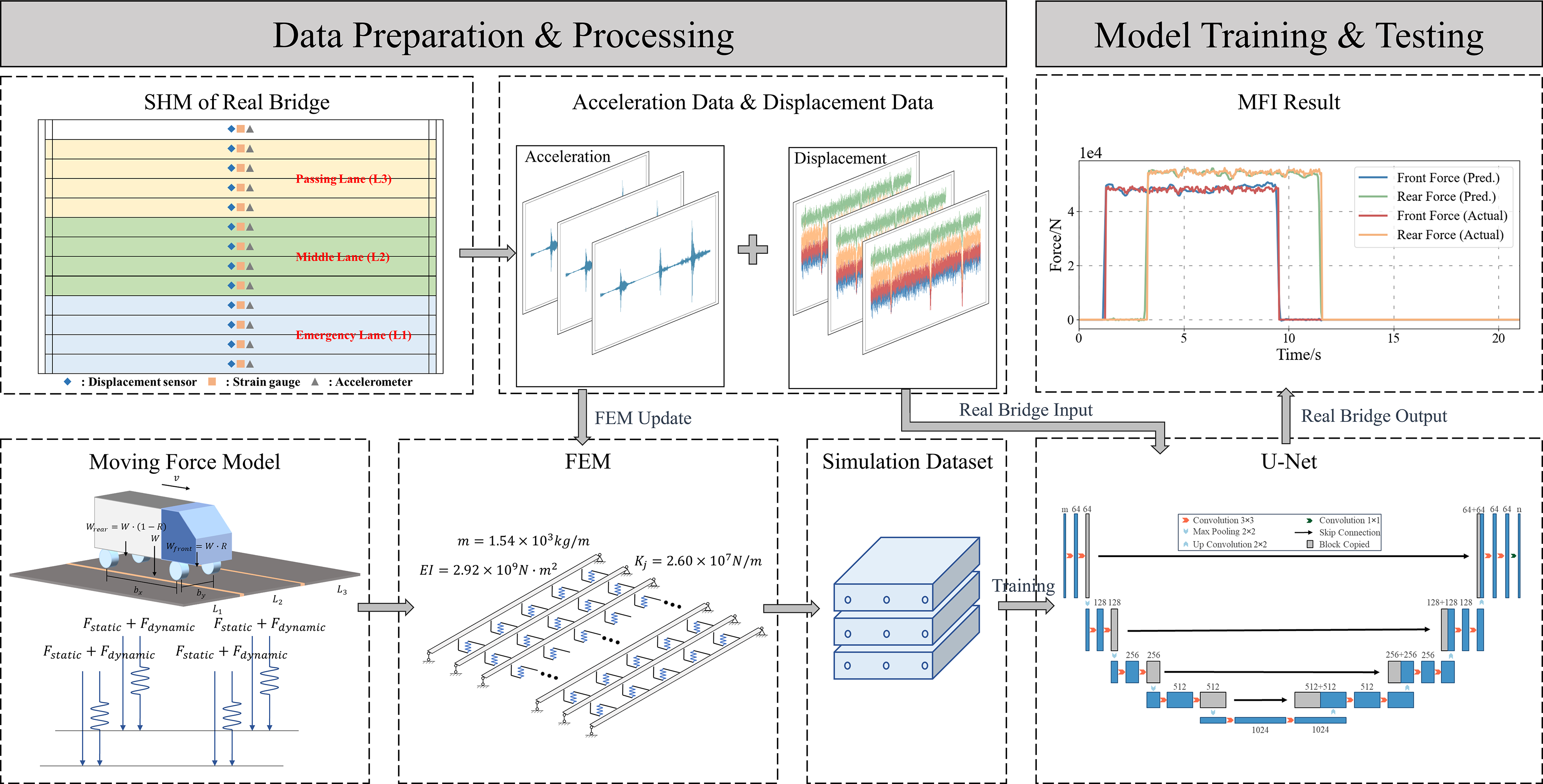

U-shaped network

The purpose of this study is to identify the time-history of moving vehicle forces, which include both global static components and localized dynamic fluctuations. Therefore, a model is required that can capture global trends while preserving fine-scale temporal variations. U-Net is well suited for this task due to its ability to combine deep semantic features with shallow structural information.

U-Net is a convolution-based encoder–decoder architecture widely used in computer vision and time-series mapping tasks. Its characteristic “U” shape consists of a contracting path for feature extraction and an expansive path for resolution recovery. The encoder progressively reduces the feature-map size while increasing channel depth, enabling the extraction of high-level representations and suppression of noise. The decoder restores temporal resolution through up-sampling while incorporating detailed features from earlier layers via skip connections (Fan et al., 2021).

The U-Net structure used in this paper is illustrated in Figure 2. The encoder contains four down-sampling stages, each composed of two 3 × 3 convolutions followed by a 2 × 2 max-pooling layer. The number of channels increases with depth as 64 → 128 → 256 → 512 → 1024. The decoder mirrors this structure, using 2 × 2 transposed convolutions for up-sampling. After each up-sampling step, the corresponding encoder features are concatenated through skip connections, followed by two 3 × 3 convolutions that refine the fused representation. A final 1 × 1 convolution maps the decoded features to the output channel(s). All convolution layers use ReLU activation. This configuration ensures that the network can simultaneously learn long-range temporal dependencies and localized dynamic features, making it suitable for mapping bridge displacement signals to axle-force time histories.

Figure 2.

U-Net structure used in this study.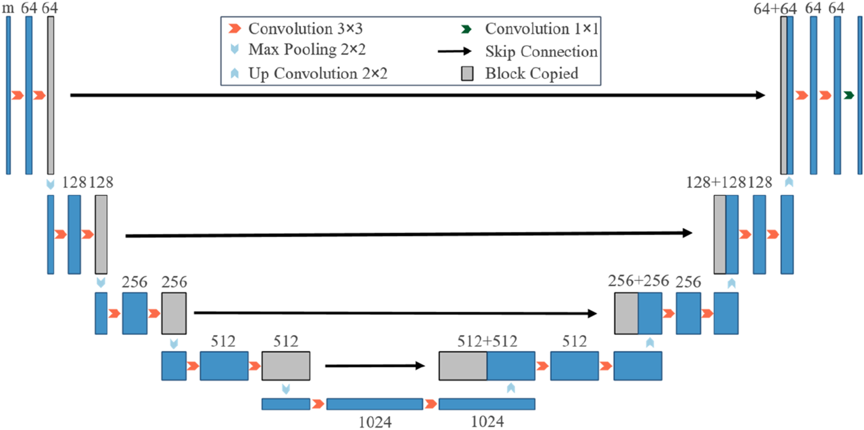

Simulation dataset generation

The training of deep learning models requires large datasets, and it is not realistic to obtain moving force identification samples from real data, so this study generates training datasets through finite element model simulation.

As illustrated in Figure 3, to simplify the interaction between the vehicle and the bridge while closely approximating real-world conditions, this study simulates the moving force load applied to the bridge during vehicle travel by adding random noise to a constant axle load, as expressed in equation (1):

F_{l o a d} (t) = F_{s t a t i c} (t) + F_{d y n a m i c} (t)

(1)

Where

F_{l o a d} (t)

represents the force applied by the vehicle to the bridge in real-time;

F_{s t a t i c} (t)

represents the static component of

F_{l o a d} (t)

, which is equal to the axle load of the vehicle; and

F_{d y n a m i c} (t)

represents the dynamic component of

F_{l o a d} (t)

, which depends on factors such as the vehicle’s axle load, road roughness, and vehicle damping characteristics. In this study, the dynamic component is simplified as a combination of multiple sine waves and random white noise, as expressed in equation (2):

F_{d y n a m i c} (t) = F_{s t a t i c} \cdot \sum_{i = 1}^{n} A_{i} \sin (ω_{i} t) + F_{w h i t e n o i s e} (t)

(2)

Where

F_{s t a t i c} \cdot \sum_{i = 1}^{n} A_{i} \sin (ω_{i} t)

represents the main part of the dynamic component. The amplitude

A_{i}

reflects the magnitude of the dynamic variation relative to the static axle load, which reflects the road surface roughness. Since detailed road-roughness data of the test bridge are not available,

A_{i}

is selected within

[0.01, 0.15]

based on engineering judgement so that the resulting dynamic-to-static load ratio is consistent with typical dynamic load coefficients reported for truck axles in the literature (Buhari et al., 2013). The angular frequency

ω_{i}

is strongly related to the vehicle’s natural vertical vibration characteristics. In this study,

ω_{i}

is set within

[2 π, 10 π]

rad/s (

[1, 5]

Hz), which covers the typical sprung-mass body-bounce and ride frequencies of road vehicles (generally 1–3 Hz) (Aye et al., 2024). Higher-frequency engine or tire vibrations are not modeled explicitly because their contribution to bridge deflection is negligible. The number of sinusoidal terms

n

is typically set between three and 5, which is sufficient to represent the low-frequency content of vehicle-induced loads while maintaining computational simplicity. Finally,

F_{w h i t e n o i s e} (t)

denotes the added white noise that simulates random fluctuations in the vehicle load.

Figure 3.

Refined axle force calculation model and Simplified axle force calculation model.

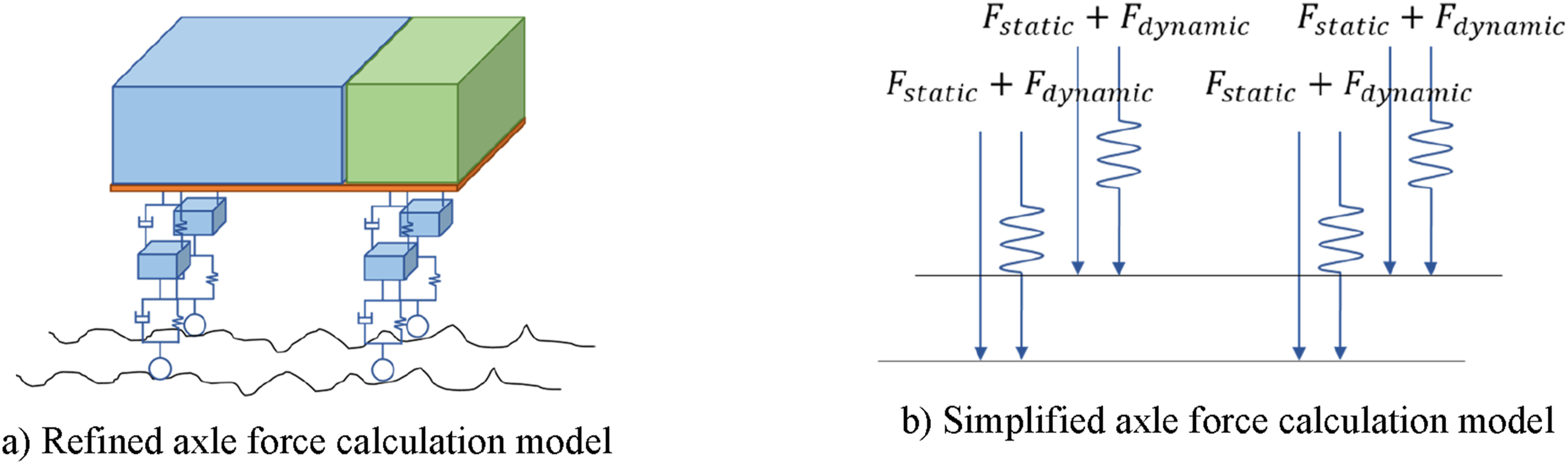
In order to simulate the various vehicle loads that the bridge may be subjected to during operation, this study considers random traffic flow under different combinations of axle load, axle spacing, vehicle width and vehicle speed, and simulates the travel of these vehicles on different lanes. For simplification, all vehicles are modeled as two-axle vehicles. The Newmark method is used to calculate the response of the bridge under random traffic flow with a time step of 0.02 s. The vertical displacement at the mid-span location of the bridge is extracted to generate the dataset.

Model training and evaluation strategy

The design of effective model training and evaluation strategies is essential to ensure the performance and generalization capability of the proposed moving vehicle load identification model. This section describes the input–output configuration, data preprocessing, and training strategy of the U-Net.

The input and output settings of the U-Net are defined as follows:

1) Input: The network input consists exclusively of structural response data, namely the mid-span vertical displacement time histories of 13 girders, resulting in 13 input channels. Each channel corresponds to one girder. For the simulation dataset, each input sequence is extracted from a time window that starts 10–40 time steps before the vehicle-induced response becomes dominant, ensuring consistent sample alignment during training. The input length is fixed at 448 samples with a uniform time interval of 0.02 s, which satisfies the architectural requirements of the U-Net and fully covers the vehicle–bridge interaction process.

2) Output: Two output configurations are considered:

A single channel representing the total axle force;

Two channels representing the front and rear axle forces.

The output length is 448 samples for both configurations. Although vehicle loads are generated using four-wheel forces in the numerical simulations for higher fidelity, it is common practice in moving force identification to simplify them into front and rear axle forces, or a single total axle force, to reduce problem complexity while meeting engineering requirements.

To mitigate the influence of scale differences and ensure stable training, both input displacement data and output force data are normalized to an appropriate numerical range.

It should be emphasized that the proposed method does not require axle position, axle spacing, or axle configuration after the vehicle enters the bridge. Unlike conventional MFI approaches that rely on external detection systems to obtain real-time axle information, the proposed method only needs an input window that includes the transition from ambient vibration to vehicle-induced response. In practical deployment, this window can be initiated using a simple threshold-based trigger that detects when the bridge response exceeds the background vibration level, without knowing the exact axle-entry time. The reference timing used in the simulation is solely for generating uniformly aligned training samples and is not required in real applications.

To mitigate the impact of differences in data magnitude on the training process, all data are normalized to align their scales.

The Adam optimizer is used during training, with an initial learning rate of 0.001. Adaptive learning rate scheduling is applied, reducing the learning rate by half if the validation set performance does not significantly improve over eight consecutive epochs. This strategy enhances training efficiency, stability, and final model performance. The optimization objective is the mean square error (MSE), which is defined as equation (3).

l o s s = \frac{1}{B} {‖ [Y] - [Y_{t r u e}] ‖}_{2}^{2}

(3)

Where,

[Y]

represents the output tensor, whose shape is

B \times C \times L

, consistent with the shape of the real value

[Y_{t r u e}]

;

B

represents the batch size of training, where it takes the value of 64;

C

represents the number of channels;

L

represents the length of the data, which takes the value of 448, with a time interval of 0.02s between neighboring points; and

{‖ \cdot ‖}_{2}

represents the

L_{2}

norm.

The dataset is randomly divided into training set, validation set, and test set in the ratio of 7:2:1. The samples in the training set were used to train the U-Net after disrupting the order. During the training process, after traversing all the training samples each time and completing one round of iterations, the validation set is input into the network. The generalizability of the network is evaluated by calculating the loss on the validation set, and an early stopping mechanism is employed to prevent the model from overfitting.

Numerical analysis

Bridge modeling

In order to verify the feasibility of the proposed moving force identification method, a finite element model is developed for numerical simulation and analysis in this study. The structural form of the finite element model is a simply supported girder bridge, which consists of 13 girders, each with a length of 20 m, $E I = 2.92 \times 10^{9} N \cdot m^{2}$ , $m = 1.54 \times 10^{3} k g / m$ , and the girders are connected by spring-simulated hinges with the stiffness of the hinges set to $2.60 \times 10^{7} N / m$ . Each girder is divided into 50 nodes, and the girder stiffnesses and masses are uniformly distributed along the longitudinal direction of the bridge. The finite element model is shown in Figure 4(a). The damping of the bridge structure is simulated by Rayleigh damping and the first order damping ratio is set to 2%. The mid-span displacement data of each girder is extracted for moving force identification.

Figure 4.

Finite element model and schematic illustration of random traffic flow vehicle parameters.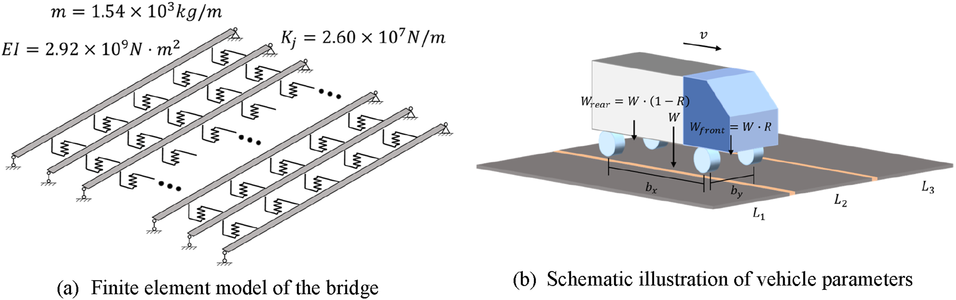

According to the simplified axle force calculation method described in Section 2.2, this study simulates random traffic flow by considering vehicles of different types traveling at various speeds and lanes. The vehicle parameters involved include the total axle weight

W

, the front axle weight ratio

R

, the front and rear axle spacing

b_{x}

, the left and right wheel spacing

b_{y}

, the vehicle speed

v

, and the driving lane

L

. A schematic illustration of these vehicle parameters in random traffic flow is shown in Figure 4(b). The front axle weight ratio

R

controls the distribution of the vehicle weight between the front and rear axles and is introduced to simulate different axle load configurations. Since common trucks generally have heavier rear axles, the value of

R

is limited to no greater than 0.5. In the numerical simulations, vehicle passages on the different driving lane were generated with equal probability to ensure a balanced distribution across lanes. Based on random combinations of these parameters, a total of 27,000 simulation samples were generated. The corresponding parameter ranges adopted in the dataset construction are summarized in Table 2.

Table 2.

Ranges of parameters used for generating random traffic flow.

Total axle weight $W$ (t)	Front axle weight ratio $R$	Front and rear axle spacing $b_{x}$ (m)	Left and right wheel spacing $b_{y}$ (m)	Speed $v$ (km/h)	Driving lane $L$
$[10, 35]$	$[0.3, 0.5]$	$[4, 7.5]$	$[2.3, 2.5]$	$[15, 65]$	${1, 2, 3}$

The actual bridge is always subject to random environmental excitation and traffic excitation, so in order to simulate the initial vibration state of the vehicles before they enter the bridge, each vehicle is first allowed to drive over the bridge with an excitation vehicle before going on the bridge, and the target vehicle passes over the bridge after the excitation vehicle has exited. The excitation vehicle’s passage is set at time 0 seconds, while the target vehicle’s passage occurs at 6.5 seconds. The wheel force time curve and the response time curve recorded in a case study are shown in Figure 5.

Figure 5.

Wheel force and response time history curve.

U-Net training and evaluation

The displacement responses and corresponding moving force time histories during each simulated vehicle passage are extracted to construct the dataset for training the U-Net. The model is trained for 100 epochs, and the loss curves for the two output configurations are shown in Figure 6. The training loss converges to a low level, indicating effective model fitting. Although the validation loss exhibits noticeable fluctuations during the early training stage, it gradually stabilizes and approaches the training loss after approximately 50 epochs, suggesting satisfactory generalization performance. To ensure optimal generalization, the model corresponding to the minimum validation loss is selected for subsequent analysis.

Figure 6.

Loss curves during training under different output conditions.

All model training was performed offline using the PyTorch framework on a workstation equipped with a single NVIDIA RTX 4070 Ti Super GPU. For the numerical simulation dataset consisting of approximately 27,000 samples, the U-Net model converged in about 100 training epochs with a batch size of 64, requiring approximately 114 minutes of training time. After training, the trained model is applied to new displacement response data in a feed-forward manner, and the inference time required to process a single vehicle passage is on the order of milliseconds, indicating that near real-time application is feasible.

Numerical simulation results

The model after training is used to test 2700 samples in the test set, and the Relative Percentage Error (RPE) RPE index is used to evaluate the accuracy of the axle force. The formula for calculating the RPE index is as follows:

RPE = \frac{{‖ F_{t r u e} - F_{i d e n t i f i e d} ‖}_{2}}{{‖ F_{t r u e} ‖}_{2}} \times 100 %

(4)

where

F_{t r u e}

represents the real-time force vector,

F_{i d e n t i f i e d}

represents the identified-time force vector, and

{‖ \cdot ‖}_{2}

is the

L_{2}

. norm.

The average loss and RPE on the test set for the two output configurations are summarized in Table 3, indicating that the proposed model achieves satisfactory identification accuracy in both cases. For both metrics, the total axle force output yields lower loss and RPE values than the front–rear axle force output, reflecting the higher difficulty associated with simultaneously identifying individual axle forces. Representative identification results are shown in Figure 7, demonstrating that the model can accurately capture vehicle entry and exit events as well as track the time-varying force evolution during bridge traversal.

Table 3.

Performance of the model on the test set.

Different cases	Mean loss	Mean RPE(%)
Outputs are total axial forces	0.369	9.170
Outputs are front and rear axle forces	0.413	10.58

Figure 7.

Identification results under different output conditions.

Sensitivity analysis

Influenced by environmental factors, monitoring data often contain varying levels of noise. Consequently, it is crucial to assess the model’s robustness to noise interference. Without altering the training and validation sets, this study introduces varying levels of noise into the inputs of the test set to evaluate the model’s sensitivity to noise.

Taking the total axle weight output as an example, white noise at levels of 0%, 2%, 5%, and 10% was added to the test set inputs to examine the model’s response to noise interference, while keeping the training and validation sets unchanged. The performance of the model is summarized in Table 4. The results indicate that as the noise level increases, both the mean identification error and the dispersion of the identification error rise. When the noise level reaches 10%, the mean loss and mean RPE are 0.703 and 12.763%, respectively.

Table 4.

Performance of the model under different measurement noise levels.

Case	Noise level(%)	Mean loss	Mean RPE(%)
N1	0	0.369	9.170
N2	2	0.391	9.460
N3	5	0.493	10.612
N4	10	0.703	12.763

In addition to noise sensitivity, the robustness of the model to sensor malfunction was also examined. In practice, missing channels are common in SHM systems due to intermittent failures. Therefore, numerical tests were conducted by removing selected displacement channels and retraining the model using reduced input dimensions. Three cases were evaluated: all 13 sensors available (baseline), 11 sensors available (removing channels 6 and 13), and 9 sensors available (removing channels 1, 5, 9, and 13). The results are summarized in Table 5.

Table 5.

Performance of the model under different sensor availability conditions.

Case	Available sensors	Missing sensors	Mean loss	Mean RPE(%)
S1	1–13	None	0.369	9.170
S2	1–5, 7–12	6, 13	0.377	9.253
S3	2–4, 6–8, 10–12	1, 5, 9, 13	0.384	9.298

The results show that the identification accuracy decreases only slightly when up to four sensors are removed, with the mean RPE increasing by less than 0.13 percentage points. This indicates that the proposed method is not highly sensitive to partial sensor loss and remains effective as long as a minimum number of displacement channels are available.

Real-world bridge verification

Bridge description

This study validates the applicability of the proposed method through a full-scale vehicle experiment on a real bridge. Figure 8 shows the side view and cross-sectional design of the test bridge. The bridge is an eight-span simply supported girder bridge, and the first span is selected as the test section. It consists of 13 precast hollow slab beams, each 20 m long, with a width of 1.0 m and a height of 0.85 m. The total bridge width is 13.5 m, accommodating three traffic lanes (passing lane, middle lane, and emergency lane). Photoelectric deflectometer targets are installed at the mid-span of each beam to measure displacement, with a sampling frequency of 33 Hz. In addition, accelerometers and strain gauges are installed at the mid-span locations.

Figure 8.

Overview of the test bridge and sensor deployment.

Vehicle experiment and data analysis

Experimental design

The vehicles used in the field experiment include three different trucks: Truck A (two axles), Truck B (three axles), and Truck C (four axles). Their vehicle profiles and axle spacings are shown in Figure 9. For Trucks B and C, the spacing between the first two axles and between the last two axles is relatively small. As discussed in Section 2.3, accurately identifying the dynamic load of each individual axle is generally challenging. To simplify the identification task, the first two axles and the last two axles are each treated as a single equivalent force, whose magnitude is taken as the sum of the corresponding axle loads and whose position is defined as the midpoint between the axles. The front axle load, rear axle load, and total axle load were measured separately, and the corresponding data are summarized in Table 6.

Figure 9.

Trucks used in the experiment.

Table 6.

Properties of the truck.

Truck ID	Weight (t)			Axle spacing (m)
Truck ID	Front axle weight	Rear axle weight	Total axle weight	Axle spacing (m)
Truck A	5.335	10.150	15.485	5.35
Truck B	11.790	13.395	25.185	5.7
Truck C	10.720	20.020	30.740	6.275

The experiment consisted of 12 rounds of truck tests, involving different types of trucks traveling at varying speeds on different lanes. The design of the truck experiment is shown in the Figure 10.

Figure 10.

Design of truck test schemes for each round.

Monitoring data analysis

The bridge is instrumented with photoelectric deflection gauges to measure mid-span displacement. The gauges have a measurement range of 0–600 mm and a sampling interval of 0.03 s. The measurement accuracy is ± 0.1 mm within 30 m and ±0.2 mm within 50 m. The displacement responses recorded during the truck tests are shown in Figure 11. As can be observed, the raw displacement data contain considerable noise and exhibit baseline drift, resulting in noticeable deviations from the numerical simulation results.

Figure 11.

Raw displacement data from the truck test.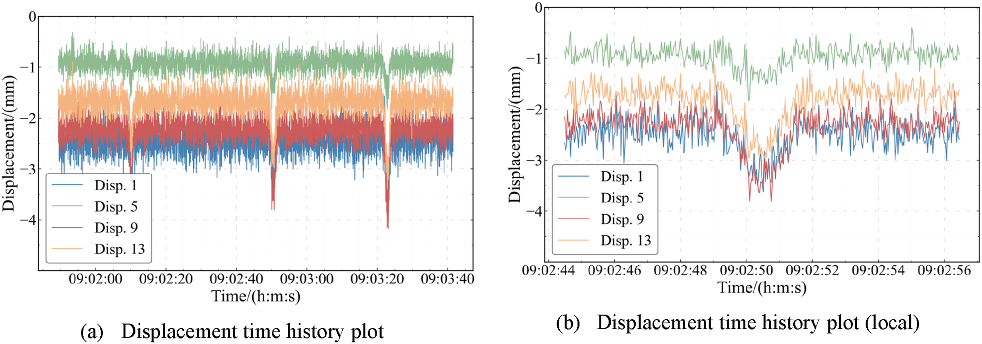

The bridge is also instrumented with accelerometers installed at the mid-span of each beam. The accelerometers operate at a sampling frequency of 50 Hz, with a measurement range of ±20 $m / s^{2}$ . The bridge natural frequencies and corresponding mode shapes identified using the FFT and FDD methods are shown in Figure 12. Notably, the identification of the bridge’s modes indicates that the peaks around 3 Hz in the power spectral density plot do not correspond to the first-order modes of the bridge. Instead, they represent the frequencies associated with traffic loads and other external influences.

Figure 12.

The natural frequency and mode of the bridge.

MFI of real bridge

Establishment and update of FEM

Based on the design documents of the bridge, the finite element model of the bridge is established. The specific parameters of the finite element are as follows: the modulus of elasticity of the beam $E = 3.45 \times 10^{10} N / m^{2}$ , the stiffness $E I = 2.92 \times 10^{9} N \cdot m^{2}$ , the material density is $2400 k g / m^{3}$ , the damping of the bridge structure is simulated by Rayleigh damping, and the first-order damping ratio is set to 2%. Each beam is divided into 50 nodes. Due to the small size of the hinge joint, it is assumed that the hinge transmits only shear force. This shear force transmission is modeled by placing springs between adjacent beams, which couple only the vertical degrees of freedom. The vertical, transverse and torsional degrees of freedom are constrained at one end of each beam, and the longitudinal axial degrees of freedom are constrained at the other end, thereby simulating simply supported boundary conditions. Since the stiffness of the hinge join cannot be obtained from the design file, it is optimized and updated based on the measured data. This optimization process involves adjusting the hinge stiffness to match the calculated natural frequencies of the model with the measured frequencies. The optimization procedure is expressed by equation (5):

K_{j} = argmin (F (K_{j})) = argmin (\sum_{i = 1}^{m} | f_{i}^{F E M} - f_{i}^{m} |)

(5)

where

K_{j}

represents the stiffness of the hinge obtained from the finite element update,

f_{i}^{F E M}

represents the

i - th

frequency of the finite element model, and

f_{i}^{m}

represents the

i - th

frequency calculated from the monitoring data.

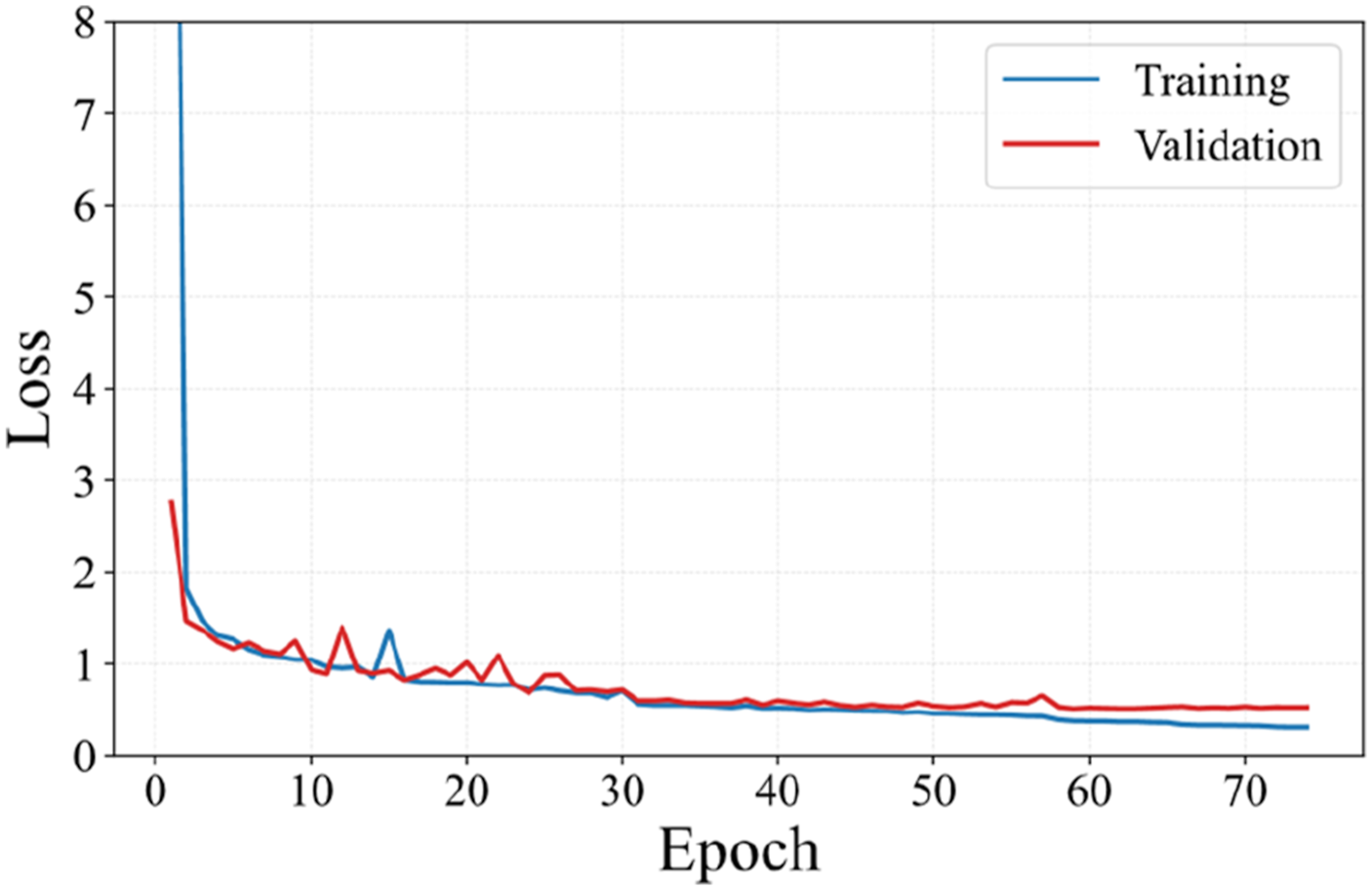
In the optimization process, the stiffness of each hinge is assumed to be the same, as all the hinges are designed with identical parameters and materials. The grid search method is employed to find the optimal hinge stiffness within a specified range, with the search range set to $[1, 4] \times 10^{7} N / m$ , and a value interval of $0.2 \times 10^{7} N / m$ . The search range is determined based on the calculated hinge stiffness of a hollow slab girder bridge similar to the test bridge structure, as reported in the literature (Gong et al., 2024). The final hinge stiffness, $K_{j}$ , is determined to be $2.6 \times 10^{7} N / m$ .

Subsequently, the method described in Section 2.2 was used to simulate random traffic flow and generate an MFI dataset corresponding to the real bridge, consisting of 27,000 samples. However, due to measurement noise and sensor errors, displacement data obtained from real bridges differ substantially from numerical simulation results. To improve the generalization performance of the model when applied to field data, noise is therefore introduced into the simulated displacement data, as expressed below:

\tilde{d} (t) = d (t) + \sum_{i = 1}^{n} B_{i} \sin (ϖ_{i} t + φ_{i}) + η (t)

(6)

Where:

\tilde{d} (t)

and

d (t)

represent the displacement data after and before processing, respectively,

\sum_{i = 1}^{n} B_{i} \sin (ϖ_{i} t + φ_{i})

and

η (t)

denote the added sine wave noise and white noise. The U-Net model is trained using the dataset with added noise, and the corresponding loss and accuracy curves during training and validation are shown in Figure 13. As observed, the model converges after 70 epochs.

Figure 13.

The loss and accuracy curves during training and validation.

Identification results

Since the sampling frequency of the displacement data collected from the real bridge test is 33.33 Hz, while the data from the numerical simulation has a sampling frequency of 50 Hz, and considering the significant noise in the raw displacement data, it is necessary to upsample and denoise the real bridge displacement data before using it for moving force identification. The noise reduction process uses the wavelet transform algorithm to remove the noise, and the basis function takes the db4 wavelet basis. Since the frequency range of the response data of research concern is roughly within 6 Hz, the number of decomposition layers is set to be $L = \log_{2} (f_{s} / f_{\min}) = \log_{2} (50 / 6) \approx 3$ . Additionally, a baseline correction algorithm based on a moving average filter is applied to remove low-frequency drift in the displacement data. Since the duration of vehicle passage is relatively short, temperature-induced or long-term environmental variations can be neglected within this time window, making the moving average approach sufficient for baseline removal.

After preprocessing, the input data sequence for each truck test is extracted starting from a short interval prior to the vehicle-induced response becoming distinguishable from background vibration. In practice, the beginning of the input window is determined directly from the measured displacement by detecting a noticeable increase above the ambient noise level, without using any axle-detection equipment or vehicle information. A fixed-length window of 448 time steps is then used as the model input for all tests.

Since the time-history axle forces of the test vehicles cannot be directly measured, static load values are used as references to evaluate the identification performance. The total vehicle weight measured by the weighbridge is taken as the ground truth (

g = 9.8 m / s^{2}

), while the mean value of the identified force time history is regarded as the identified axle force, and the sum of the identified axle forces is taken as the identified total force. The corresponding statistical results are summarized in Table 7. It should be noted that although the test design specified target vehicle speeds of 20 km/h, 40 km/h, and 60 km/h, the actual speeds could only be approximately controlled. For data analysis purposes, the vehicle speeds are therefore assumed to be equal to the specified target values.

Table 7.

Summary of identification results.

Rounds of truck tests	Truck ID	Lane ID	Speed (km/h)	Identified force(kN)	True force (kN)	RPE (%)
1	A	L2	20	165.714	151.753	9.20
	B	L2	20	246.295	246.813	0.21
	C	L2	20	285.256	301.252	5.31
2	A	L2	40	153.786	151.753	1.34
	B	L2	40	254.415	246.813	3.08
	C	L2	40	287.756	301.252	4.48
3	A	L2	60	167.323	151.753	10.26
	B	L2	60	277.270	246.813	12.34
	C	L2	60	288.479	301.252	4.24
4	A	L3	20	169.372	151.753	11.61
	B	L3	20	261.721	246.813	6.04
	C	L3	20	305.590	301.252	1.44
5	A	L3	40	133.634	151.753	11.94
	B	L3	40	225.513	246.813	8.63
	C	L3	40	360.147	301.252	19.55
6	A	L3	60	123.527	151.753	18.60
	B	L3	60	249.651	246.813	1.15
	C	L3	60	295.438	301.252	1.93
7	A	Cross L1-L2	20	148.824	151.753	1.93
	B	Cross L1-L2	20	254.045	246.813	2.93
	C	Cross L1-L2	20	299.746	301.252	0.50
8	A	Cross L1-L2	40	159.492	151.753	5.10
	B	Cross L1-L2	40	234.324	246.813	5.06
	C	Cross L1-L2	40	310.681	301.252	3.13
9	A	Cross L1-L2	60	151.996	151.753	0.16
	B	Cross L1-L2	60	261.005	246.813	5.75
	C	Cross L1-L2	60	284.894	301.252	5.43
10	A	Cross L2-L3	20	154.181	151.753	1.60
	B	Cross L2-L3	20	260.881	246.813	5.70
	C	Cross L2-L3	20	277.935	301.252	7.74
11	A	Cross L2-L3	40	170.388	151.753	12.28
	B	Cross L2-L3	40	258.709	246.813	4.82
	C	Cross L2-L3	40	284.141	301.252	5.68
12	A	Cross L2-L3	60	167.323	151.753	10.26
	B	Cross L2-L3	60	277.270	246.813	12.34
	C	Cross L2-L3	60	288.479	301.252	4.24

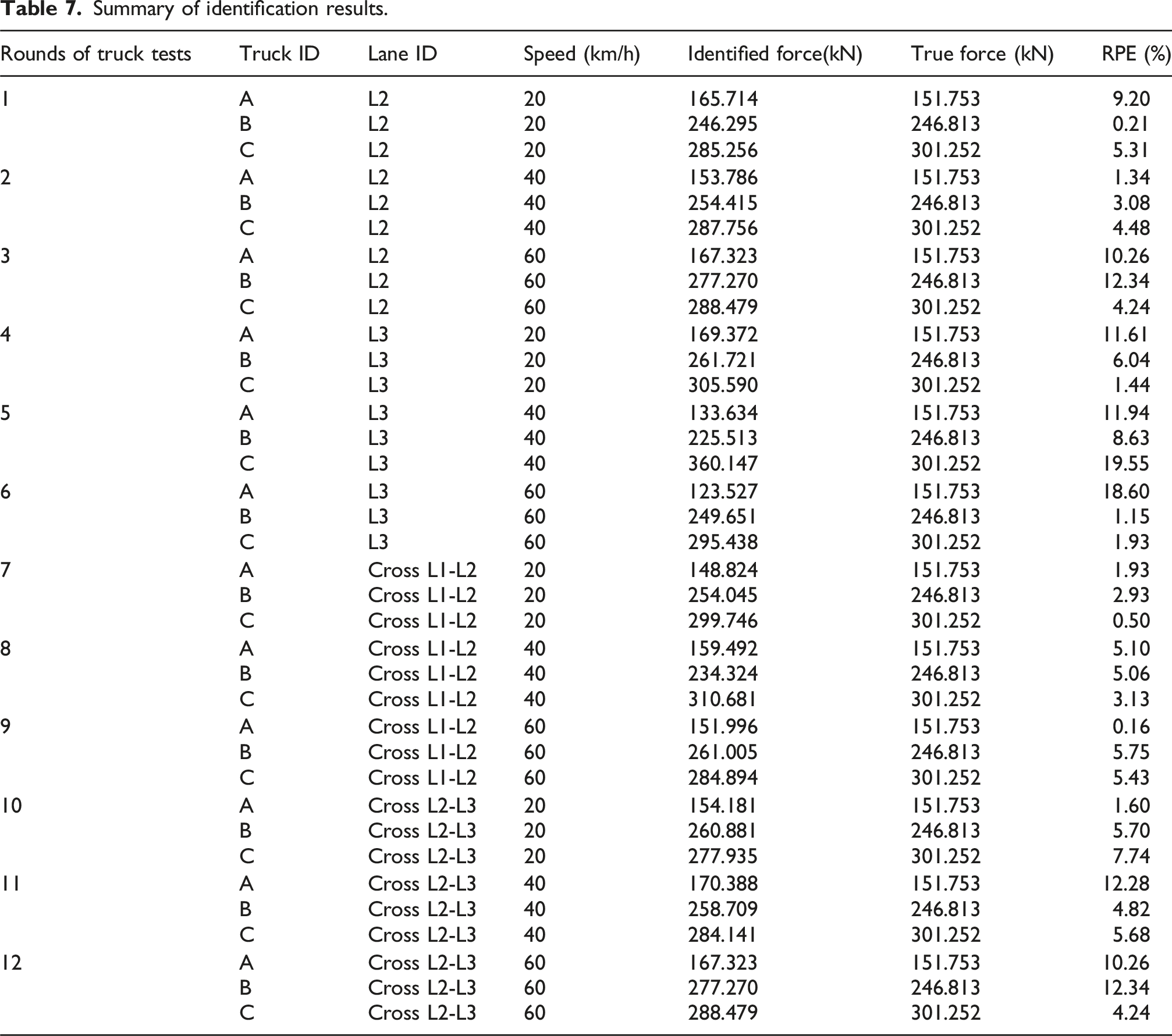
In a total of 36 tests, the mean RPE index of identified result is 6.28%. The box plots of RPE for trucks A, B and C are shown in Figure 14(a). As the axle force rises, the error of the identification tends to decrease. This can be attributed to the fact that a higher axle force leads to larger displacements in the bridge structure, making it easier for the model to identify the axle force. The box plots of the RPE at different speeds are shown in Figure 14(b). It can be observed that there is no significant difference in RPE as speed increases, indicating that the model is robust to changes in speed.

Figure 14.

Identification results for different conditions.

Representative time-history results of the MFI predictions are shown in Figure 15. The model accurately identifies the axle forces and detects the vehicle entry and exit events with good temporal precision. A transient force overshoot is observed when the front axle first enters the bridge, where the predicted force briefly exceeds the reference value before returning to a stable level. This behavior is likely caused by impact effects during vehicle entry, which can be induced by expansion joints or surface irregularities and may result in dynamic loads exceeding the static vehicle weight.

Figure 15.

Truck test identification results (total axle force).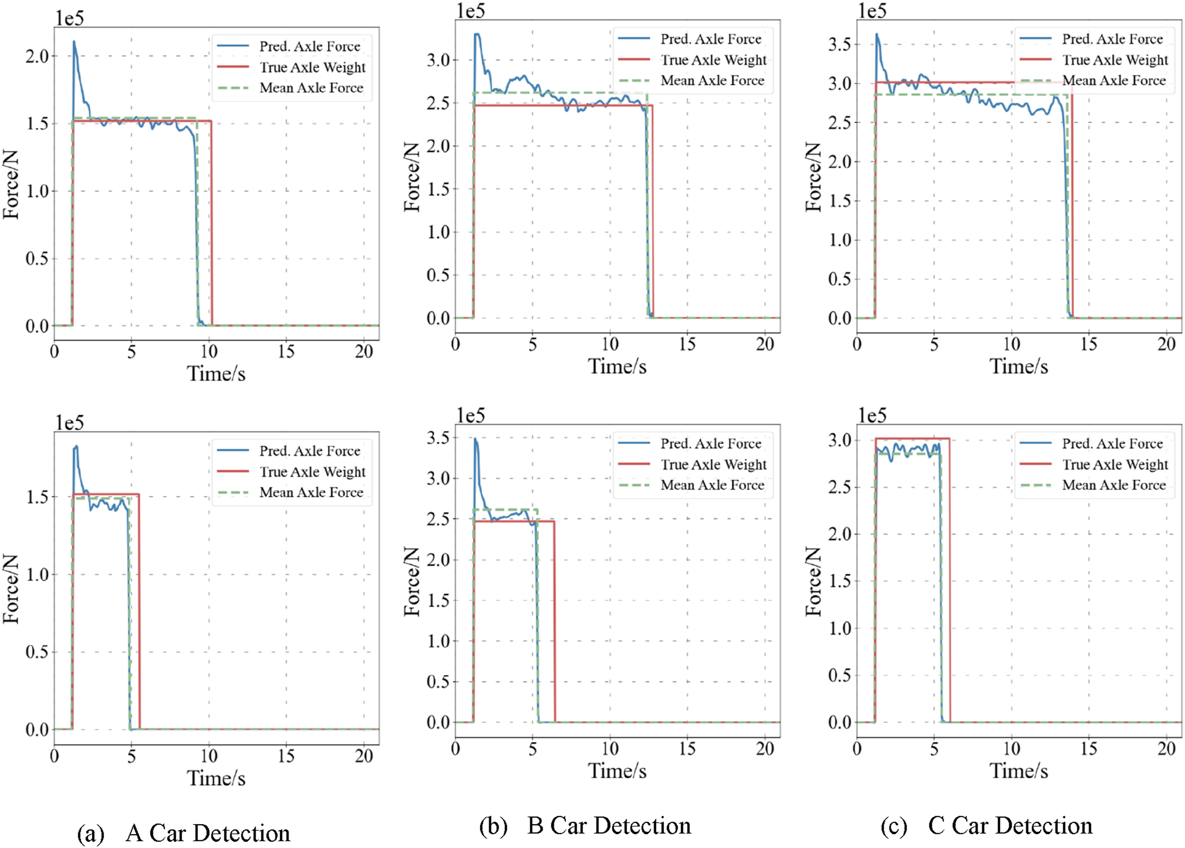

The performance of the model in identifying front and rear axle forces is further evaluated, with representative results shown in Figure 16. Compared with total axle force identification, individual axle force predictions exhibit larger errors and fluctuations. This is expected, as only a limited portion of the displacement response is dominated by a single axle, whereas the front and rear axles act simultaneously for most of the vehicle passage. Accurately separating individual axle forces from noisy measurements therefore remains a more challenging task.

Figure 16.

Truck test identification results (front and rear axle forces).

Conclusions

Based on a U-Net architecture, this paper proposes a moving force identification (MFI) method that relies solely on structural monitoring data and does not require prior knowledge of axle information, such as real-time axle positions or axle spacing. Bridge mid-span displacement responses are used as inputs to predict dynamic axle forces. The method is validated through numerical simulations covering a wide range of axle weights, axle spacings, and vehicle speeds to assess robustness. Furthermore, full-scale tests on a real bridge using three different trucks demonstrate the feasibility of the proposed approach for practical engineering applications.

The numerical results show that the U-Net model can accurately identify both total axle force and dynamic axle forces for the front and rear axles based on displacement data, even when axle information is unknown. The model demonstrates strong robustness against noise interference. The results of the actual bridge experiment show that the mean error of axle load identification is 6.28%. Even when the vehicle speed reaches up to 60 km/h, the proposed model is still able to identify dynamic axle loads with good accuracy.

However, there are some limitations in this study. First, the vehicle models considered are simplified to two-axle vehicles and single-vehicle loading scenarios, which may not fully reflect the complexity of real bridge operations under dense traffic conditions. Extending the proposed method to account for multi-vehicle loading scenarios will be an important topic of future research. In addition, although displacement data are used in this study, displacement responses can in principle be derived from acceleration measurements. Since acceleration sensors are generally lower in cost and easier to install than displacement sensors, developing a moving force identification method based entirely on acceleration data is another key direction for future work.

Footnotes

ORCID iDs

Cheng Pan

Fengzong Gong

Funding

The authors disclosed receipt of the following financial support for the research, authorship, and/or publication of this article: This study is supported by the National Natural Science Foundation of China (52411540031; 52278313), and the National Key Research and Development Program of China (2025YFF0519200).

Declaration of conflicting interests

The authors declared no potential conflicts of interest with respect to the research, authorship, and/or publication of this article.

References

Aye

Win

Swe

WWM

, et al. (2024) Vibration analysis of suspension System for 3DOF quarter car model with tire damping. International Journal of Mechanical Engineering and Robotics Research 13: 196–204. https://doi.org/10.18178/ijmerr.13.2.196-204

Buhari

Rohani

Abdullah

(2013) Dynamic load coefficient of Tyre forces from truck axles. Applied Mechanics and Materials 405-408: 1900–1911. https://doi.org/10.4028/www.scientific.net/amm.405-408.1900

Burnos

Gajda

(2016) Thermal property analysis of axle load sensors for weighing vehicles in weigh-in-motion System. Sensors 16: 11. https://doi.org/10.3390/s16122143

Cao

(2025) Overview of the construction scheme for the Jiasong Highway Bridge over the Huangpu River. Prestress Technology 3: 73–87. https://doi.org/10.59238/j.pt.2025.03.006

Chan

THT

Law

Yung

, et al. (1999) An interpretive method for moving force identification. Journal of Sound and Vibration 219: 503–524. https://doi.org/10.1006/jsvi.1998.1904

Chang

Tang

Xin

, et al. (2025) Low-complexity real-time detection Transformer for identifying bridge vehicle loads. Computer-Aided Civil and Infrastructure Engineering 40: 4485–4506. https://doi.org/10.1111/mice.70061

Chen

Chan

THT

(2017) A truncated generalized singular value decomposition algorithm for moving force identification with ill-posed problems. Journal of Sound and Vibration 401: 297–310. https://doi.org/10.1016/j.jsv.2017.05.004

Fan

Hao

(2021) Dynamic response reconstruction for structural health monitoring using densely connected convolutional networks. Structural Health Monitoring-an International Journal 20: 1373–1391. https://doi.org/10.1177/1475921720916881

Feng

Sun

Feng

(2015) Simultaneous identification of bridge structural parameters and vehicle loads. Computers & Structures 157: 76–88. https://doi.org/10.1016/j.compstruc.2015.05.017

10.

Gong

Lei

Xia

(2024) Real-time damage identification of hinge joints in multi-girder bridges using recursive least squares solution of the characteristic equation. Engineering Structures 300: 15. https://doi.org/10.1016/j.engstruct.2023.117147

11.

Hao

Xie

(2019) The identification technology of vehicle weight based on bridge strain time-history curve. Advances in Structural Engineering 22: 1606–1616. https://doi.org/10.1177/1369433218823487

12.

Jian

Xia

Lozano-Galant

, et al. (2019) Traffic sensing methodology combining influence line theory and computer vision techniques for girder bridges. Journal of Sensors 2019: 15. https://doi.org/10.1155/2019/3409525

13.

Jian

Lai

Xia

, et al. (2022) A robust bridge weigh-in-motion algorithm based on regularized total least squares with axle constraints. Structural Control and Health Monitoring 29: 21. https://doi.org/10.1002/stc.3014

14.

Jian

Xia

Chatzi

, et al. (2024) Bridge influence surface identification using a deep multilayer perceptron and computer vision techniques. Structural Health Monitoring-an International Journal 23: 1606–1626. https://doi.org/10.1177/14759217231190543

15.

Kawakatsu

Aihara

Takasu

, et al. (2019) Deep sensing approach to single-sensor vehicle weighing System on bridges. IEEE Sensors Journal 19: 243–256. https://doi.org/10.1109/jsen.2018.2872839

16.

Kim

Lee

Park

, et al. (2009) Vehicle signal analysis using artificial neural networks for a Bridge weigh-in-motion System. Sensors 9: 7943–7956. https://doi.org/10.3390/s91007943

17.

Law

Chan

THT

Zeng

(1997) Moving force identification: a time domain method. Journal of Sound and Vibration 201: 1–22. https://doi.org/10.1006/jsvi.1996.0774

18.

Pan

Liu

(2017) Identification of moving vehicle forces on bridge structures via moving average Tikhonov regularization. Smart Materials and Structures 26: 16. https://doi.org/10.1088/1361-665x/aa7a48

19.

Pan

Liu

, et al. (2018) Moving force identification based on redundant concatenated dictionary and weighted l₁-norm regularization. Mechanical Systems and Signal Processing 98: 32–49. https://doi.org/10.1016/j.ymssp.2017.04.032

20.

Qiao

Chen

Xue

, et al. (2015) The application of cubic B-spline collocation method in impact force identification. Mechanical Systems and Signal Processing 64-65: 413–427. https://doi.org/10.1016/j.ymssp.2015.04.009

21.

Richardson

Jones

Brown

, et al. (2014) On the use of bridge weigh-in-motion for overweight truck enforcement. International Journal of Heavy Vehicle Systems 21: 83–104. https://doi.org/10.1504/ijhvs.2014.061632

22.

Sujon

Dai

(2021) Application of weigh-in-motion technologies for pavement and bridge response monitoring: State-of-the-art review. Automation in Construction 130: 16. https://doi.org/10.1016/j.autcon.2021.103844

23.

Tang

Xin

Jiang

, et al. (2022) Fast identification of random loads using the transmissibility of power spectral density and improved adaptive multiplicative regularization. Journal of Sound and Vibration 534: 117033. https://doi.org/10.1016/j.jsv.2022.117033

24.

Wang

(2025) Investigation on the application of external prestressing technology in Bridge. Prestress Technology 4: 89–94. Available at: https://doi.org/10.59238/j.pt.2025.04.008

25.

Wang

Zhang

Pan

, et al. (2025) Deflection influence line identification under moving vehicle based on variational modal decomposition and B-spline basis function. Advances in Structural Engineering.

26.

Huang

(2017) Development of sensor validation methodologies for structural health monitoring: a comprehensive review. Measurement 109: 200–214. https://doi.org/10.1016/j.measurement.2017.05.064

27.

Chan

THT

(2003) Moving force identification based on the frequency-time domain method. Journal of Sound and Vibration 261: 329–349. https://doi.org/10.1016/s0022-460x(02)00991-4

28.

Chan

THT

Zhu

(2008) A MOM-based algorithm for moving force identification: part II - experiment and comparative studies. Structural Engineering & Mechanics 29: 155–169. https://doi.org/10.12989/sem.2008.29.2.155

29.

Cai

Deng

(2016) State-of-the-art review on bridge weigh-in-motion technology. Advances in Structural Engineering 19: 1514–1530. https://doi.org/10.1177/1369433216655922

30.

Zeng

Feng

, et al. (2024) Deep learning-based identification of vehicular moving forces for bridges without axle configurations. Engineering Structures 304: 16. https://doi.org/10.1016/j.engstruct.2024.117646

31.

Zhang

Xie

Peng

, et al. (2021) A deep neural network-based vehicle re-identification method for bridge load monitoring. Advances in Structural Engineering 24: 3691–3706. https://doi.org/10.1177/13694332211033956

32.

Zhu

Law

(2002) Moving loads identification through regularization. Journal of Engineering Mechanics-Asce 128: 989–1000. https://doi.org/10.1061/(asce)0733-9399(2002)128:9(989)

33.

Zhu

Law

(2006) A state space formulation for moving loads identification. Journal of Vibration and Acoustics-Transactions of the Asme 128: 509–520. https://doi.org/10.1115/1.2202149

34.

Zuo

Ren

(2019) Vehicle weight identification for a bridge with multi-T-girders based on load transverse distribution coefficient. Advances in Structural Engineering 22: 3435–3443. https://doi.org/10.1177/1369433219854548