Pipe failure prediction model based on periodic pipe wall thickness measurement using electromagnetic acoustic resonance

Abstract

This study proposes a numerical model to predict pipe failure based on periodic non-destructive inspections using electromagnetic acoustic resonance (EMAR). A total of 149 artificially corroded samples that simulated flow-assisted corrosion were prepared; 27 of them were plates, and others were from pipes of various dimensions. The samples were measured using EMAR, and the thicknesses of the samples were evaluated based on the fundamental resonance frequency. The results of the evaluations were compared with the actual thicknesses measured by a caliper gauge to quantify the uncertainty in pipe wall thickness evaluation. Numerical evaluations were performed to predict pipe failure probability in the future based on the results of periodic EMAR measurements. Three scenarios of pipe thickness reduction were considered, and each scenario assumed that pipe thickness measurements by EMAR were performed every five years. The actual pipe wall thickness, which is not necessarily the same as the EMAR evaluations, is estimated as a probability density function using the Bayesian approach proposed in an earlier study by the authors. Whereas this study considers only pipe rupture, the results of numerical simulations support the validity of the model especially when the corrosion rate is not constant.

Keywords

nondestructive testing and evaluation electromagnetic acoustic transducer flow assisted corrosion pipe wall thinning management wall thinning

Introduction

Pipe wall thinning is among the most important aging degradations in many industries. A pipe wall is gradually thinned due to the interaction with fluids it carries, which is known as flow-assisted or flow-accelerated corrosion (FAC). Thus, pipes need to be properly repaired or replaced to avoid failure or rupture. Many studies have been performed so far to reveal the mechanisms of FAC.^1,2,3 However, quantitatively estimating the corrosion rate is still challenging. While computational fluid dynamics, combined with other computational physics,^3,4,5 would enable to estimate corrosion rates, performing such simulations in a practical environment is not always feasible because it requires to know all influential parameters in advance. Several recent studies have proposed the use of machine learning for estimating corrosion rates.^6,7 However, sufficient data for training is only sometimes available, which hampers the application of machine-learning-based approaches. Thus, evaluating pipe wall thickness by applying periodic non-destructive tests to measure actual pipe wall thickness is necessary in practice to predict the remaining life of the pipe and take proper action.^8,9,10

Electromagnetic acoustic transducer (EMAT) is an effective method for the monitoring of pipe wall thickness as it can be operated remotely without couplant. It is a well-established technique; several commercial instruments are already available in the market. Several studies have reported that EMAT works well at high temperatures,^11,12,13 which would be a large advantage in monitoring pipes carrying high-temperature fluids. One of the recent major research directions of EMAT is to generate guided waves.^14,15 Using guided waves enables quick inspection of a long pipe. Another research direction is to enhance the signal-to-noise ratio because the accuracy of EMAT is not always as clear as that of an ultrasonic thickness gauge because of its low energy conversion ratio. One of the options to address this issue is to use the fact that signals of EMAT become very large when the thickness of the target is an integer multiple of half of the wavelength. Thus, confirming frequencies when signals are maximized provides information on the thickness of the target,^16,17 which is known presently as electromagnetic acoustic resonance (EMAR). Several groups have reported the applicability of EMAR to pipe wall thickness monitoring^18,19,20; earlier studies by the authors have demonstrated that properly analyzing the results of periodic pipe wall thickness measurements by EMAR enables quantitative prediction of when pipe wall thickness reaches a certain threshold.^21,22 In contrast, it is preferable that residual life be discussed based on the probability of pipe failure from the viewpoint of risk-based maintenance to allocate resources properly and reasonably.

On the basis of the background above, this study develops a probabilistic analysis model that can predict the probability of pipe failure taking the uncertainty of measurement and pipe material toughness into consideration based on periodic EMAR measurement results. This study prepared artificially corroded carbon steel samples and performed EMAR measurements to quantify the accuracy of EMAR. Subsequently, the model was applied to the analyses of virtual periodic EMAR evaluations of pipe wall thickness that gradually became thinner. The results of the analyses supported the effectiveness of the model, especially when corrosion rate was not constant.

Pipe wall thickness measurement using EMAR

Sample preparation

This study prepared 149 artificially corroded carbon steel samples that simulated flow-assisted corrosion of general carbon steel pipes carrying liquid. Table 1 summarizes the specifications of the samples. The “Type” of the samples indicates the specification of the samples following Japan Industrial Standards (JIS). Samples with various shapes were prepared to avoid results obtained from becoming specific to a particular pipe dimension. The sizes of the samples are sufficiently large compared to the size of the EMAR probe used in this study.

Table 1.

Sample specifications.

Type	Shape	Initial thickness	Outer diameter	Dimensions	Number of samples
SS400	Plate	6.0 mm	—	120 mm × 70 mm	27
STPG50A Sch80	1/3 pipe	5.5 mm	60.5 mm	120 mm × 120 deg.	25
STPG90A Sch20	1/4 pipe	4.5 mm	101.6 mm	120 mm × 90 deg.	13
STPG90A Sch40	1/6 pipe	5.7 mm	101.6 mm	50 mm × 60 deg.	59
STPG90A Sch60	1/4 pipe	7.0 mm	101.6 mm	120 mm × 90 deg.	13
STPG150A Sch20	1/6 pipe	5.5 mm	165.2 mm	120 mm × 60 deg.	11

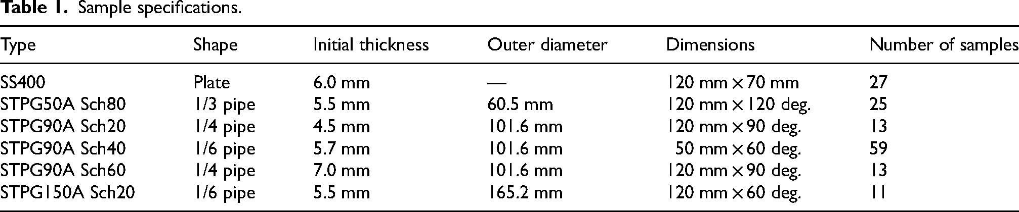
The samples were corroded by soaking in iron(III)-chloride-based etchant (H-1000A, Sunhayato Corp., Tokyo, Japan) at 50 °C. The duration of this corrosion test ranged from 51 to 727 h so that the samples had various degrees of corrosion. The corrosive solution was renewed and the surfaces of the samples were polished manually using a metallic scrubber approximately every 100 h. During the corrosion test, the surfaces of the samples were masked by vinyl tape so that only one of the surfaces, the inner surface in the case of the pipe samples, was corroded.

The corroded surfaces of the samples were uneven. The maximum arithmetical mean height, calculated with a cut-off wavelength of 0 mm using a 3D measuring macroscope (VR-3000, KEYENCE Corp., Osaka, Japan), was several hundred micrometers. It was difficult to confirm the dependence of the roughness on the duration of the corrosion test. The thickness of each sample was measured using a caliper gauge at the center of the sample where EMAR was performed.

Evaluating the thicknesses of the samples by using EMAR

Figure 1 illustrates the experimental setup to measure EMAR signals and one of the samples. An EMAR probe consisting of two samarium-cobalt magnets and a single-layer racetrack was operated by a high-powered pulser-receiver (RPR-4000, RITEC, RI, USA). Each magnet measured 10 mm × 20 mm × 20 mm, and they were arranged so that their poles were opposed to each other. Because of the directions of the magnetic field generated by the magnets and the induced eddy currents, ultrasonic transverse waves are generated. Note that the ultrasonic wave used in this study is not guided waves but the conventional bulk wave. The bottom surfaces of the magnets were curved so that the racetrack coil fits the surface of the samples. The signals were recorded by a PC after analog-to-digital conversion using an oscilloscope (DPO4104, Tektronix, OR, USA) as a function of frequency. The frequency used in this study ranged from 1.0 MHz to 4.0 MHz with a pitch of 500 Hz. The thickness of each sample was evaluated based on the fundamental resonance frequency obtained using the superposition of the n-th compression technique^18,23 The speed of shear wave necessary for calculating the thickness was 3266.7 m/s, which was obtained by measuring uncorroded flat samples with a known thickness.

Figure 1.

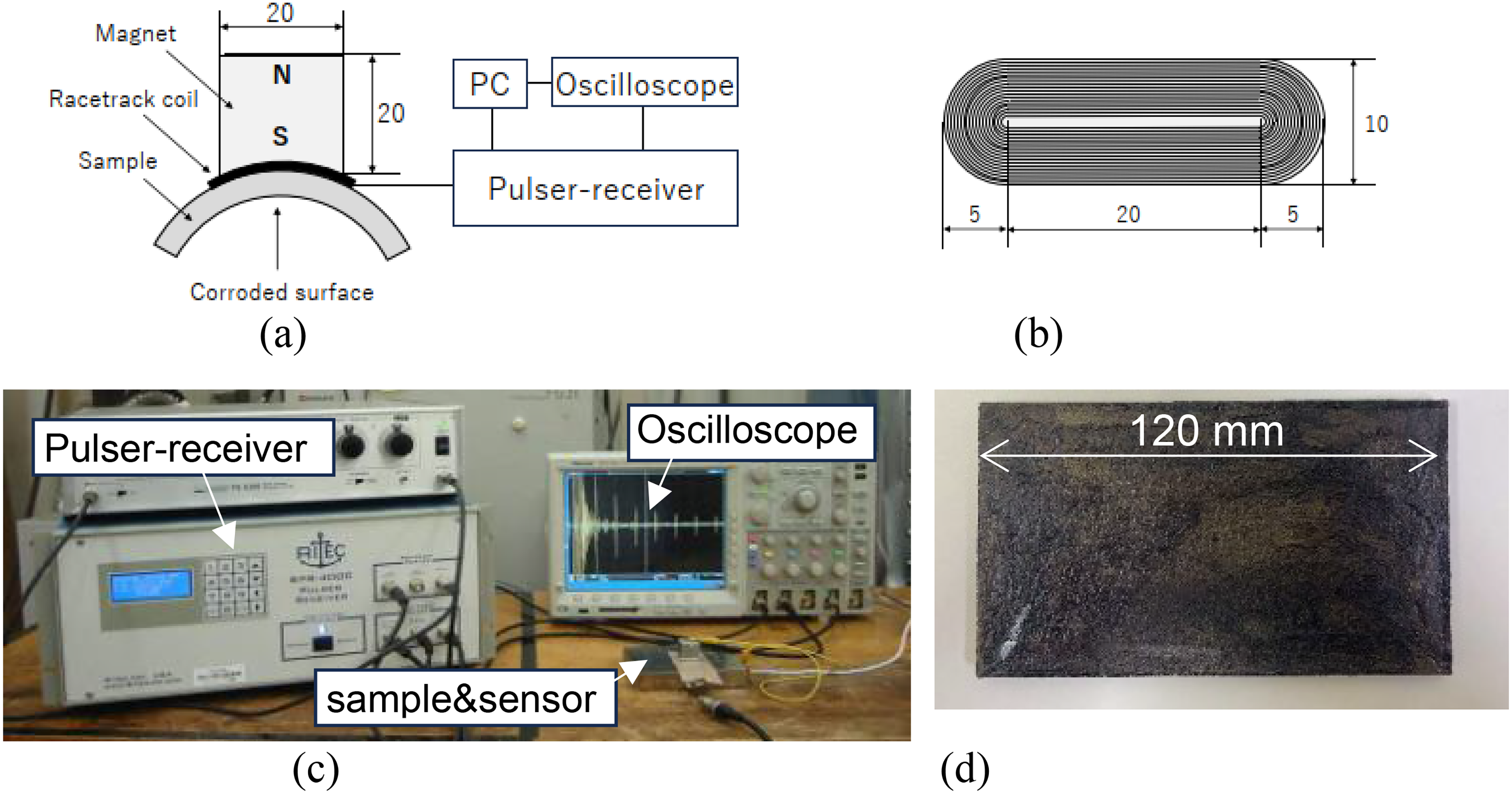
Experimental setup. (a) arrangement. (b) racetrack coil. (c) testing system. (d) one of the samples (SS400).

Results

Figure 2 presents examples of measured EMAR signals. Most of the samples provided clear signals as shown in Figure 2(a). The clear peaks almost equally spaced represent resonance frequencies. In contrast, signals from some of the samples were not so clear as shown in Figure 2(b). Whereas the most probable reason for this is the material property of the sample, further studies are necessary to reveal what causes such large difference in signals. Figure 3 shows the relationship between the estimated and true thicknesses obtained by processing measured signals using the superposition of the n-th compression technique. 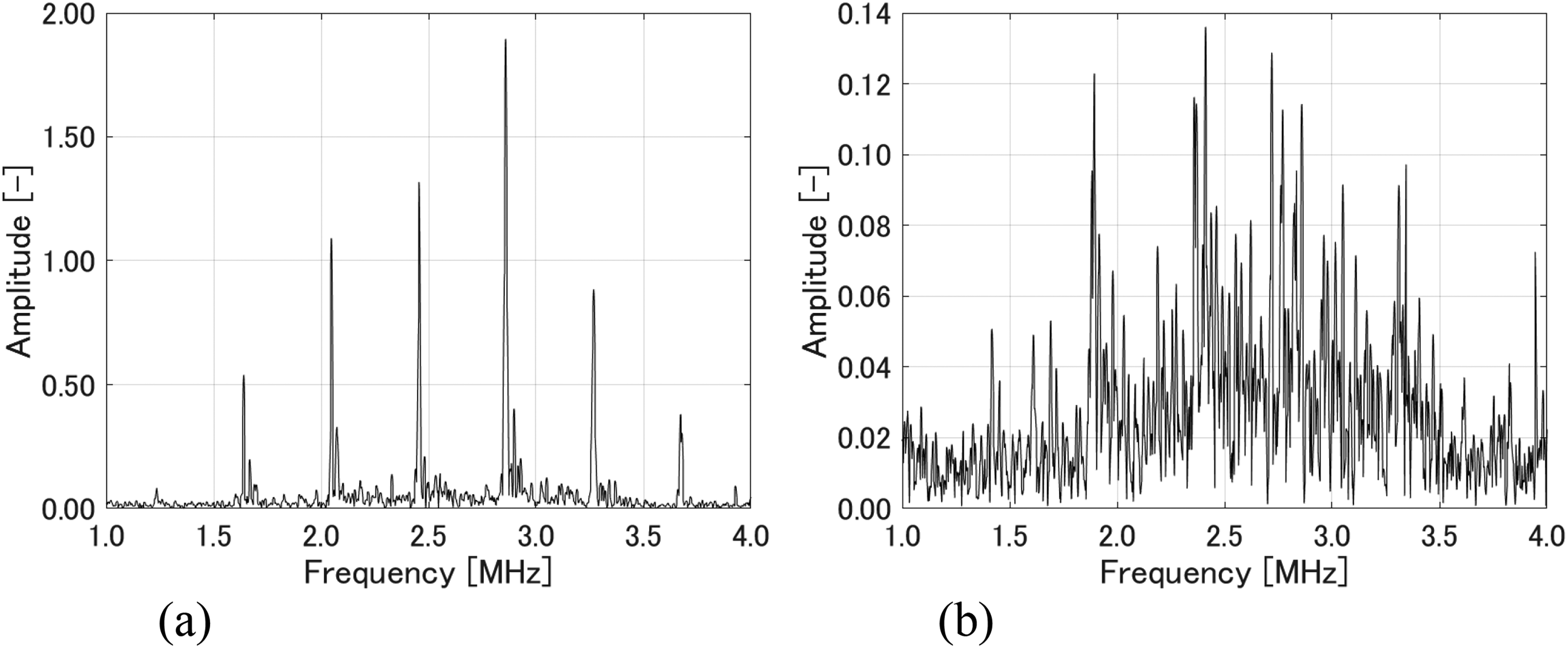The solid and broken lines represent the results of linear regression analysis with an assumption that error follows a normal distribution, namely mean and $\pm 1$ standard deviation, respectively. The correlation coefficient and root mean square error were 0.96 and 0.18 mm, respectively. The figure indicates that the error in thickness evaluation would depend on the type of sample. However, intensive statistical analyses could not confirm the correlation of the error on the geometrical parameters of the samples including the radius of the curvature. This implies that other uncontrollable factors, such as the electromagnetic properties of the samples, had a dominant effect on the precision of EMAR. Thus, the regression lines shown in the figure were used in subsequent analyses to represent error in thickness evaluation.

Figure 2.

Measured EMAR signals. (a) with clear resonances. (b) with unclear resonance.

Figure 3.

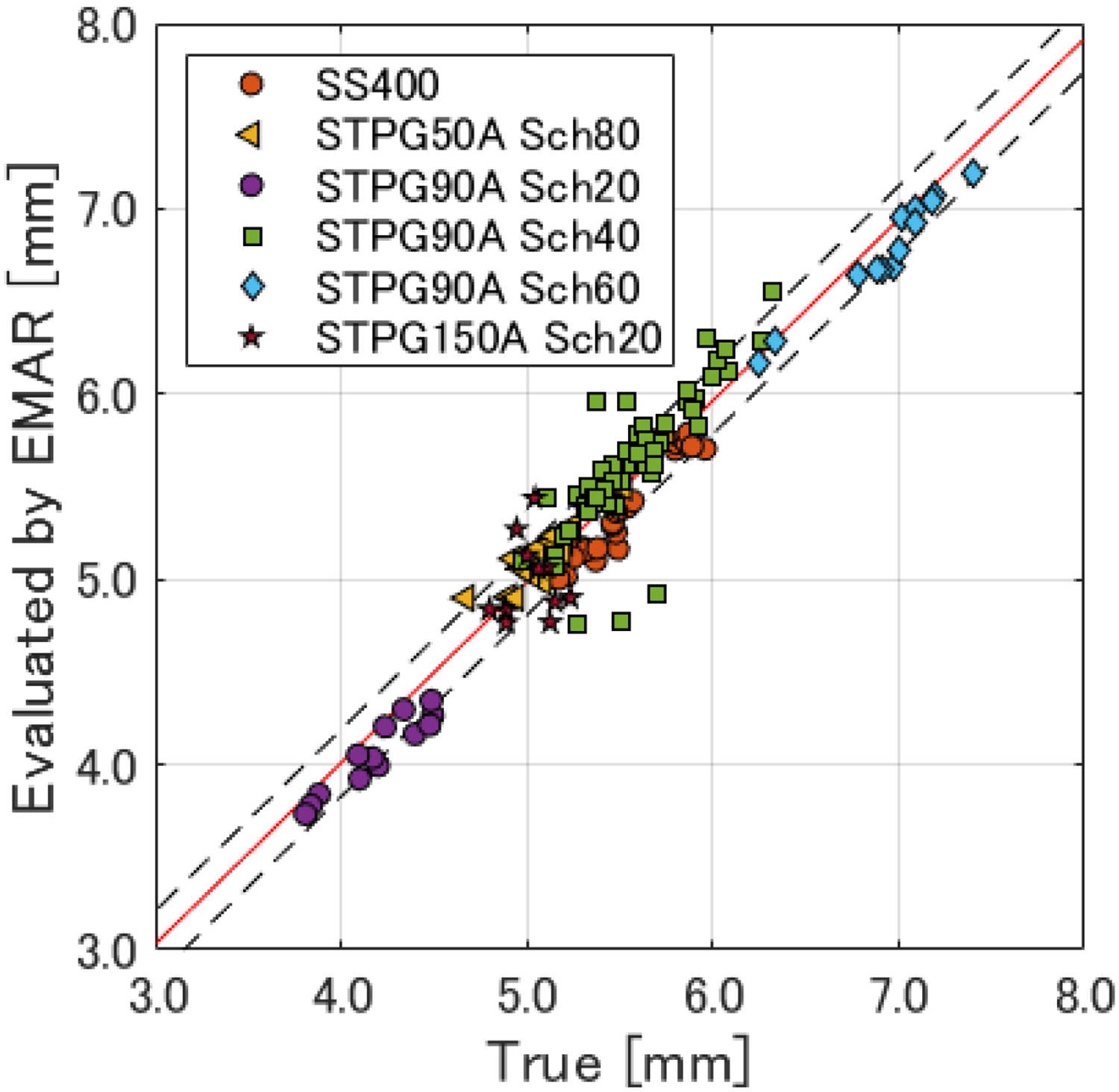
Comparison between evaluated and true thicknesses of the samples.

Developing a pipe failure prediction model

Numerical model

This study considered virtual pipes subjected to gradual thickness reduction. There are various forms of pipe failure, and quite a few models have been proposed to evaluate pipe failure probability. The choice of a model mainly depends on factors to consider in calculating the probability, such as load condition and type of failure, as summarized well in a recent review.²⁴ Because developing a model to consider new factors is beyond the scope of this study, this study evaluated pipe failure probability considering only pipe burst due to internal pressure and adopted Wesley's criteria proposed for carbon steel pipes.^25,26 Specifically, the pipe burst pressure, 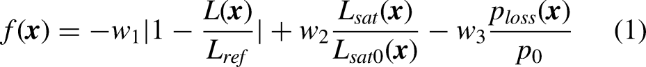$P_{f}$ , used in this study is given as

P_{f} = σ_{f} \frac{T_{0} - W (t)}{(r_{0} + W (t)) (1 + 0.25 ε_{f})},

(1)

where

σ_{f}

T_{0}

W (t)

r_{0}

, and

ε_{f}

are failure stress, initial pipe wall thickness, the loss of pipe wall thickness as a function of time (t), the initial inner radius of the pipe, and median hoop strain at failure.²¹ This study set

σ_{f}

to 85% of the ultimate tensile stress and assumed that the ultimate tensile stress follows a normal distribution with a mean of 500 MPa and standard deviation of 52 MPa.^25,26 The probability of pipe burst is given as the probability that

P_{f}

becomes lower than the internal pressure,

P_{i n t}

. The parameters of the pipe are summarized in Table 2.

Table 2.

Specification of the pipe.²⁵

Parameter	Value
Shape	straight
Initial thickness, $T_{0}$	12.7 mm
Initial inner radius, $r_{0}$	228 mm
Ultimate tensile stress, $σ_{U T S}$	N(500, 52²) MPa*
Internal pressure, $P_{i n t}$	10.0 MPa
Median hoop strain at failure, $ε_{f}$	3.7%

* $N (μ, σ^{2})$ : normal distribution with a mean of $μ$ and standard deviation of $σ$ .

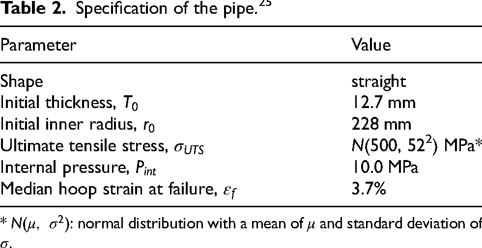
Figure 4 presents the three scenarios of pipe wall thickness reduction considered in this study. A pipe with an initial thickness of 12.7 mm is gradually thinned to 7.37 mm that provides a failure probability of 1%. Case 1 simulates the case where a large corrosion rate appears at the beginning of the operation, while Cases 2 and 3 has a constant and gradually increasing corrosion rates, respectively. It should be noted that the time scale is not essential in the discussion hereafter.

Figure 4.

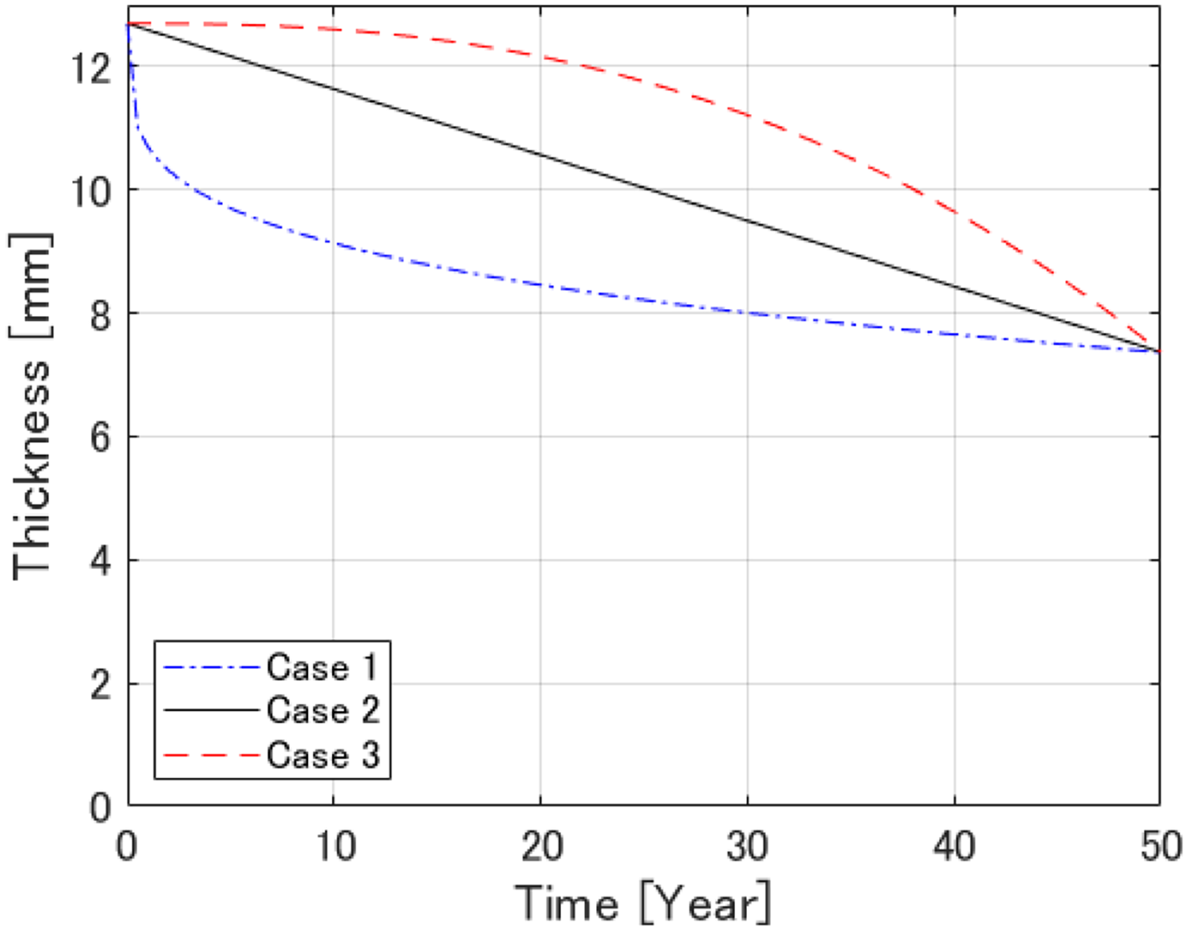
Thickness reduction.

The evaluation here assumed that EMAR measurements were performed every five years. Based on the results shown in Figure 3, this study assumed that the pipe wall thicknesses evaluated by the EMAR measurements follow a normal distribution whose mean and mean $\pm 1$ standard deviation are represented by the solid and broken lines in the figure, respectively. More specifically, this study randomly generated virtual results of EMAR thickness measurements based on the true thickness of a pipe shown in Figure 4 and the model obtained by the regression analysis; sufficient number of virtual results were generated to avoid the effect of the randomness.

Predicting the probability of pipe failure in the future

Because pipe wall thickness monotonically decreases with time, it is reasonable to assume that 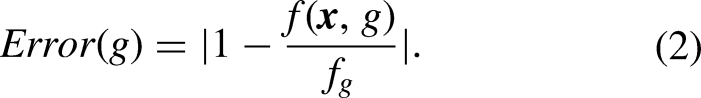$W (t)$ can be represented using two positive parameters, a and b, as

W (t) = a t^{b} .

(2)

The parameters can be estimated from the results of periodic pipe wall thickness evaluations. However, an error in thickness measurements sometimes leads to a large error in predicting the wall thickness in the future using Equation (2). Thus, this study estimates the parameters not from the results of the measurements themselves but from the maximum a posterior estimation of the Bayesian approach proposed in an early study by the authors.²² Specifically, this study assumes that if measured pipe wall thickness at the i-th inspection is $x_{i}$ , the probability that actual pipe wall thickness follows, $P (T | x_{i})$ , is given as

P (T | x_{i}) = \frac{P (x_{i} | T) P (T)}{\int P (x_{i} | T) P (T) d T},

(3)

where

P (x_{i} | T), T

, and

P (T)

stand for the likelihood, pipe wall thickness, and prior distribution. Because the actual relationship between the measured and true thicknesses should be unknown, this study used a normal distribution with a mean of T and a standard deviation of 1.5 times that of the regression analysis shown in Figure 3 as the likelihood. The prior distribution was calculated by extrapolating the posterior distributions of previous evaluations, while a uniform distribution was used in the first evaluation where information on the previous inspection was unavailable. More detail of the prior, including its mathematical formulation, can be found in.²² While the prior can be calculated at any time, this study assumed that shifting the mean of the posterior distribution of the Bayesian approach along Equation (2) predicts the pipe wall thickness in the future. This is because the prior was designed to have a conservatively large standard deviation so that the probability that the present pipe wall thickness differs largely from that of the previous inspection result is not completely excluded. Once the probability density function that pipe wall thickness follows is obtained, the failure probability is calculated as

\int_{- \infty}^{\infty} P (T | \vec{x}) F (T) d T,

where

\vec{x},

and

F (T)

are measured pipe wall thicknesses and the probability that a pipe burst pressure becomes lower than the internal pressure when pipe wall thickness is T, respectively. The measured pipe wall thicknesses are represented by a vector because the approach takes the history of the measured thicknesses through the Bayesian updates.

For comparison, the pipe failure probabilities were evaluated using a conventional model based on the linear regression analyses as well. The conventional model also predicted the loss of pipe wall thickness using Equation (2), while the parameters were estimated by the thicknesses evaluated by the linear regression analysis of the results of the thickness measurements. Because the standard deviation of the linear regression analysis was sometimes too large, the probability of failure was calculated directly from the predicted thickness, without integrating the probability as Equation (3).

This study evaluated pipe failure probabilities 10 years ahead and compared them with the true ones. The number of Mote-Carlo trials to randomly generate virtual results of EMAR thickness measurement was 1000. The virtual results of EMAR thickness measurements that the two models used were the same.

Results

Figure 5 presents the true and predicted failure probability obtained by the model proposed in this study. Because the evaluation here uses random variables, the graphs show several percentiles of the predicted failure probability obtained by the Monte-Carlo simulations. The graphs demonstrate that the proposed model could predict the true failure probability in the future reasonably well. The result of Case 1 overestimates the failure probability especially at 20 and 25 years, which is due to the sudden decrease in the pipe wall thickness at the beginning as shown in Figure 4. This overestimation is relaxed as time passes, i.e., with the number of measurements.

Figure 5.

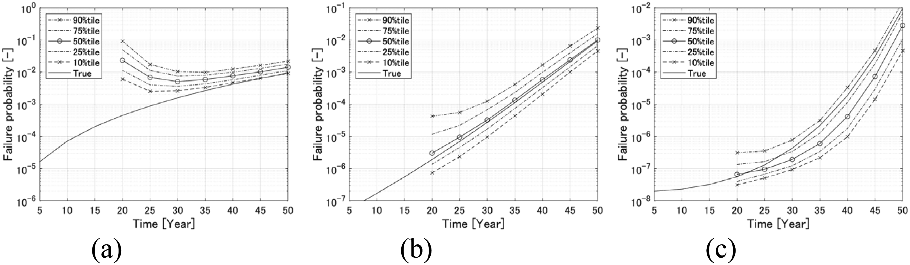
True and predicted pipe failure probability using the proposed model. (a) Case 1. (b) (a) Case 2. (c) Case 3.

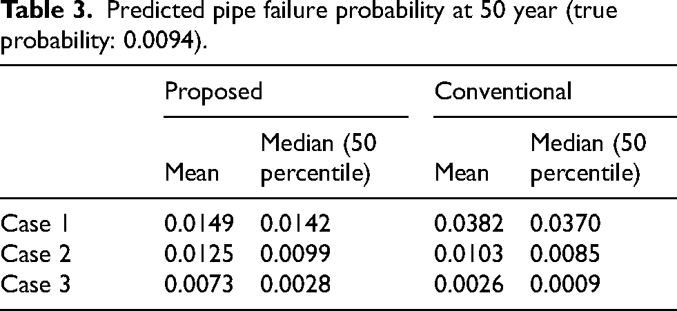
Figure 6 shows the results of the pipe wall thickness predictions using the conventional model. Five latest measurement results were used for the regression analyses to obtain the results. Comparing Figures 5 and 6 reveals that if the corrosion rate is constant, namely in Case 2, the proposed model is not so advantageous over the conventional one. This is reasonable because a linear model should fit a linear phenomenon better than a model that does not postulate the linearity. In contrast, the results demonstrate the effectiveness of the proposed model when the corrosion rate is not constant. The proposed model provided predictions closer to the true failure probability in Cases 1 and 3 than the conventional one. The large errors in predicting the failure probability at the years 20 and 25 in Case 1 are due to the large change in the corrosion rate at the early stage as shown in Figure 4. The conventional model always overestimated the failure probability because it could not “forget” the large corrosion rate in the past. In contrast, the estimation by the proposed model approaches the true one with the number of inspections. It should also be noted that the number of measurements for the regression analysis has a large effect in predicting pipe wall thickness in the future using the conventional model. A greater number leads not only to robustness against measurement error but also a larger discrepancy between the true and evaluated thicknesses when the corrosion rate is not constant; a lesser number provides opposed characteristics. It is a practical advantage that the proposed model does not require discussion on the proper number of thickness measurements. Table 3 summarizes the mean and median of the predicted pipe failure probabilities at 50 years. The table confirms that the proposed method provided failure probabilities closer to the true one, 0.0094.

Figure 6.

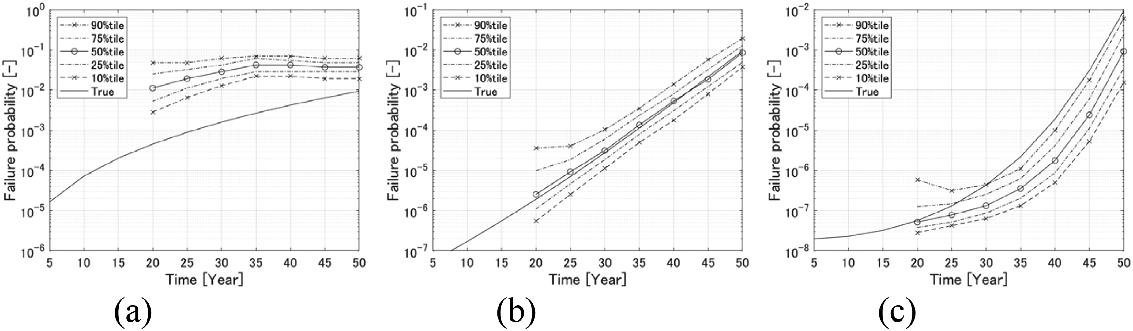
True and predicted pipe failure probability using a conventional model. (a) Case 1. (b) Case 2. (c) Case 3.

Table 3.

Predicted pipe failure probability at 50 year (true probability: 0.0094).

	Proposed		Conventional
	Mean	Median (50 percentile)	Mean	Median (50 percentile)
Case 1	0.0149	0.0142	0.0382	0.0370
Case 2	0.0125	0.0099	0.0103	0.0085
Case 3	0.0073	0.0028	0.0026	0.0009

Conclusion

This study proposed a pipe failure prediction model based on periodic pipe wall thickness measurements by EMAR. Laboratory tests were performed using 149 artificially corroded carbon steel samples with various dimensions to evaluate the precision of EMAR in pipe wall thickness measurement. Subsequent numerical analyses were performed to evaluate the effectiveness of the model, whose results demonstrated that the model is advantageous over the conventional one using linear regression analysis especially when the corrosion rate is not constant. This study assumed that the thickness of the pipe wall does not spatially change significantly. Actual defects sometimes appear more locally; and thus how sensors are positioned has a large effect on the uncertainty of the evaluation. Further studies are necessary to take this issue into account.

Footnotes

Funding

The author(s) received no financial support for the research, authorship, and/or publication of this article.

Declaration of conflicting interests

The author(s) declared no potential conflicts of interest with respect to the research, authorship, and/or publication of this article.

References

Kain

. Flow accelerated corrosion: forms, mechanisms, and case studies. Proce Eng 2014; 86: 576–588.

Khunphakdee

Chalermsinsuwan

. Review of flow accelerated corrosion mechanism, numerical anslysis, and control measures. Chem Eng Res Des 2023; 197: 519–535.

Poulson

. Predicting and preventing flow accelerated corrosion in nuclear power plant. Int J Nuclear Energy 2014; 2014: 423295. doi:10.1155/2014/423295

Madasamy

, et al. Influence of bend geometry on flow accelerated corrosion under neutral pH conditions. Eng Failure Anal 2021; 122: 105127.

Zhang

, et al. A study of flow accelerated corrosion at elbow of carbon steel pipeline by array electrode and computational fluid dynamics simulation. Corros Sci 2013; 77: 334–341.

, et al. The research progress and prospect of data mining methods on corrosion prediction of oil and gas pipelines. Eng Failure Anals 2023; 144: 106951.

Diao

Yan

Gao

. Improvement of the machine learning-based corrosion rate prediction model through the optimization of input features. Mater Des 2021; 198: 109326.

Vanaei

Eslami

Egbewande

. A review on pipeline corrosion, in-line inspection (ILI), and corrosion growth rate models. Int J Press Vessels Piping 2017; 149: 43–54.

Uchida

, et al. Improvement plant reliability based on combination of prediction and inspection of wall thinning due to FAC. Nucl Eng Des 2018; 337: 84–95.

10.

Nishiguchi

, et al. A review: Japanese pipe wall thinning management based on JSME rules and recent R&D studies performed to enhance the rules. E-J Adv Mainten 2010/2011; 2: 14–24.

11.

Burrows

Fan

Dixon

. High temperature thickness measurements of stainless steel and low carbon steel using electromagnetic acoustic transducers. NDT&E Int 2014; 68: 73–77.

12.

Zhao

, et al. Application of adaptive filtering based on variational mode decomposition for high-temperature electromagnetic acoustic transducer denoising. Sensors 2022; 22: 7042.

13.

Zhai

Liang

, et al. High-temperature EMAT with double-coil configuration generates shear and longitudinal wave modes in paramagnetic steel. NDT&E Int 2022; 125: 102572.

14.

Cawley

. Guided waves in long range nondestructive testing and structural health monitoring: principles, history of applications and prospects. NDT&E Int 2024; 142: 103026.

15.

Memon

AlHems

. Applications of EMAT generated guided waves in pipes: a review. e-J Nondestruct Testing 2023; 28: 10.

16.

Kawashima

Wright

. Resonant electromagnetic excitation and detection of ultrasonic waves in thin sheets. J Appl Phys 1992; 72: 4830.

17.

Hirao

Ogi

Fukuoka

. Resonance EMAT system for acoustoelastic stress measurement in sheet metals. Rev Sci Instrum 1993; 64: 3198.

18.

Urayama

Takagi

Uchimoto

, et al. Online monitoring of pipe wall thinning by electromagnetic acoustic resonance method. E-J Adv Mainten 2013; 5: 155–164.

19.

Chai

, et al. An acentric archimedes spiral coil for inspection of an aluminum plate with an inhomogeneous thickness. Nondestruct Test Evaluat 2023; 38: 1075–1100.

20.

Nakamoto

, et al. Pipe-wall thickness measurement at high temperature by electromagnetic acoustic transducer. In: Capova

(eds) Electromagnetic nondestructive evaluation (XVII). Amsterdam, the Netherlands, IOS Press, 2014, pp.256–262.

21.

Yusa

, et al. Probabilistic analysis of electromagnetic acoustic resonance signals for the detection of pipe wall thinning. Nondestr Test Eval 2005; 36: 1–16.

22.

Yusa

, et al. Probabilistic evaluation of EMAR signals to evaluate pipe wall thickness and its application to pipe wall thinning management. NDT&E Int 2021; 122: 102475.

23.

Sun

, et al. Data processing method for thickness measurement using electromagnetic acoustic resonance. In: Tamburrino

(eds) Electromagnetic nondestructive evaluation XXII. Amsterdam, the Netherlands, IOS Press, 2019, pp.1–6.

24.

Amaya-Gomez

, et al. Reliability assessments of corroded pipelines based on internal pressure–A review. Eng Failure Anal 2019; 98: 190–214.

25.

Japan Atomic Energy Agency. JAEA-Data/Code 2006–001.

26.

Wesley

. Interfacing systems LOCA (ISLOCA) component pressure capacity methodology and typical plant results. Nucl Eng Des 1993; 142: 209–224.