An Econometric Analysis of Revenue Diversification Among Selected Indian States

Abstract

The key objective of this article is to empirically examine the trends and determinants of revenue diversification with respect to 14 major Indian states. The findings highlight a gradual decrease in the level of revenue diversification, which has become more visible in recent years. This indicates an erratic pattern of growth in tax and non-tax revenue sources. The panel cross-sectional–autoregressive distributed lag model test results reveal a positive contribution of economic and institutional factors, as compared to political factors, toward the process of revenue diversification. Overall, it is evident that cyclical fluctuations in the major tax revenue sources, coupled with a lessened emphasis on rationalising the structure of non-tax revenue sources, seem to have had an adverse impact on the process of revenue diversification on the part of states.

JEL Classifications: H0, H1, H2, H7

Keywords

Fiscal policy revenue structure revenue diversification CS-ARDL

Introduction

Revenue adequacy refers to the availability of a sufficient level of revenue required to ensure uninterrupted public service delivery. For adequate revenue generation, proper management of the revenue structure with a diverse set of revenue sources is essential. In this direction, changes in tax policy and reform measures and differences in tax bases help diversify their revenue portfolios. Diversification is the process of changing the level of diversity of revenue mobilisation as part of mitigating the uncertainty associated with reliance on a single or a few revenue sources. Following the existing literature, diversification of revenue helps expand the tax base, reduce the fiscal stress (Shamsub & Akoto, 2004), reduce the extent of variability associated with revenue mobilisation, improve fiscal stability (Oates, 1985), besides improving the overall fiscal performance. Even to insulate sub-national governments against any external shocks, mobilizing sufficient revenue through internal sources is desirable, as it helps ensure autonomy, flexibility and accountability with respect to revenue management. Thus, tax collection from multiple sources may make governments less vulnerable to the risk associated with increased dependency on any one single source of revenue during a phase of sluggish economic activity.

In the Indian context, it becomes evident that a larger part of the states’ revenue continues to be derived from their own revenue sources. Of the total own tax revenue, more than half flows from sales tax, followed by excise, stamp and taxes on vehicles. Revenues from sales and stamps and from registration fees are relatively more elastic as compared to motor vehicle tax and excise duty, whereas revenues from state excise and motor vehicle taxes have remained relatively inelastic, even showing a consistent increase during the period of economic slowdown (MTFP, 2011, various issues).

The process of fiscal decentralization (own financial compulsion) has forced the states to improve their own source revenue mobilisation through diversifying their revenue structure and introducing fiscal reforms over time. The medium term fiscal plan (MTFP) is used for incentivising states to undertake some fiscal restructuring and institutional reforms at the subnational level. Overall, the reforms at the state level, mainly the fiscal adjustment measures, undertaken in the last decade to improve their fiscal position have helped the states improve their own-tax revenue mobilization, but they have failed to maintain consistency for a longer period (MTFP, various issues). For instance, the increasing revenue gap is a major concern haunting the Indian states (Kurian & Sushmita, 2004), as reflected by a long-term decline in the states’ own revenues from 69% in 1955–1956 to 52% in 2002–2003 (Singh, 2006). Some studies have even observed an increase in the coefficient of variation with regard to per capita own revenues over the years, resulting in a growing divergence between per capita own revenue and per capita expenditure (Chakraborty, 2014). In view of these revenue- and expenditure-led fiscal correction measures and tax reform measures undertaken at the sub-national level, it is necessary to examine the extent of reliance on different sources of revenue over time.

An analysis of the pattern and extent of revenue diversification helps analyze the variations in the changing revenue structures of states. However, because of the lesser emphasis laid on the importance of revenue diversification in the fiscal policy at the national and sub-national levels, this kind of analysis has not been attempted before in the Indian context. Therefore, the present analysis aims to explore the changes in the revenue composition, the extent and the changing trends in the revenue diversification across 14 major Indian states for the period of 1981–2017.

The structure of the article is as follows: The present study aims to assess the trends in revenue diversification across 14 major Indian states. For this purpose, the study critically assesses the changing trends in the extent of revenue diversification across the states. The study also examines the determinants of revenue diversification followed by theoretical background to revenue diversification and a brief overview of empirical studies that have examined the aspects of revenue diversification.

An Overview of Total Revenue Sources

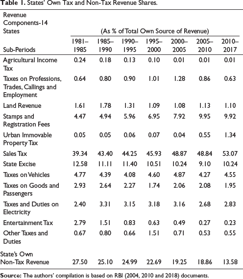
In the total revenue structure, states’ own revenue sources are broadly classified into tax and non-tax revenue sources. Tax revenue sources can be further classified into direct and indirect taxes. The revenue categories used in this analysis include taxes on income, taxes on property and capital transactions, taxes on commodities and services, and states’ own non-tax revenue. Taxes on income comprise agricultural income tax and taxes on professions, taxes on property and capital transactions comprise land revenue, stamps and registration fees and urban immovable property tax, taxes on commodities and services comprise sales tax, state excise, taxes on vehicles, taxes on goods and passengers, taxes and duties on electricity, entertainment tax and other taxes and duties.

It is evident from Table 1 that in the changing revenue structure, the contribution of sales tax accounts for more than half of own source revenue. Although sales tax predominates the period under analysis as a whole, from the first half of the 1990s, stamp duty, registration fee, entertainment tax and taxes on vehicles show an increase in their relative share over the period under their respective categories. The real estate boom, growing urbanization and increasing number of registered motor vehicles have also contributed towards revenue collection over the years. The revenue from four major state taxes, such as stamps and registration fees, sales tax, excise duty and motor vehicle tax, comprising taxes on vehicles and taxes on goods and passengers, accounts for a larger portion of the aggregate own-source revenue of the states, while receipts from interest, dividends and profits from state PSUs and income from royalties constitute a relatively larger share of the non-tax revenue. Overall, the own source revenue kitty tells a dismal story, though the states have managed to improve the ratio of own tax revenue-GSDP from 1990–1991 to 2016–2017. It is also important to notice that several low-income states have become fiscally prudent through improving their own-tax revenue, besides having a larger share in the divisible pool as compared to middle- and high-income states (Rathin Roy, 2022).

Table 1.

States’ Own Tax and Non-Tax Revenue Shares.

Revenue Components-14 States	(As % of Total Own Source of Revenue)
Sub-Periods	1981–1985	1985–1990	1990–1995	1995–2000	2000–2005	2005–2010	2010–2017
Agricultural Income Tax	0.24	0.18	0.13	0.10	0.01	0.01	0.01
Taxes on Professions, Trades, Callings and Employment	0.64	0.80	0.90	1.01	1.28	0.86	0.63
Land Revenue	1.61	1.78	1.31	1.09	1.08	1.13	1.10
Stamps and Registration Fees	4.47	4.94	5.96	6.95	7.92	9.95	9.92
Urban Immovable Property Tax	0.05	0.05	0.06	0.07	0.04	0.55	1.34
Sales Tax	39.34	43.40	44.25	45.93	48.87	48.84	53.07
State Excise	12.58	11.11	11.40	10.51	10.24	9.10	10.24
Taxes on Vehicles	4.77	4.39	4.08	4.60	4.87	4.27	4.55
Taxes on Goods and Passengers	2.93	2.64	2.27	1.74	2.06	2.08	1.95
Taxes and Duties on Electricity	2.40	3.31	3.15	3.18	3.16	2.68	2.83
Entertainment Tax	2.79	1.51	0.83	0.63	0.49	0.27	0.23
Other Taxes and Duties	0.67	0.80	0.66	1.51	0.71	0.53	0.55
State’s Own Non-Tax Revenue	27.50	25.10	24.99	22.69	19.25	18.86	13.58

Source: The authors’ compilation is based on RBI (2004, 2010 and 2018) documents.

Changed fiscal scenarios and fiscal correction measures undertaken in the last decade (FRBM, 2004) have helped the states improve their revenue mobilisation capacity in the post-reform, to a larger extent (MTFP, various issues), but there is no long-term consistency observed in this respect. It is even observed that the coefficient of variation with regard to per capita own revenues continues to persist over the years.

As part of continued tax reform, the Goods and Services Tax (GST), introduced on 1 July 2017, encompasses various taxes coming under the Union and state government’s indirect tax bases (Mukherjee, 2019). Considering that excise and stamp duties happen to be the major revenue-yielding sources in the period of transition, with more uncertainty surrounding the initial stages of implementation of the GST as a major indirect tax reform, states need to focus on other existing taxes to improve their own revenue collection. Thus, it becomes evident that state governments must mobilize additional resources, as their reliance on non-sales taxes and non-tax revenue is inevitable.

With the onset of the COVID-19 pandemic, a shortfall in states overall revenue receipts has become more evident in recent years. A larger shortfall in revenue led to the curtailment of total expenditure and even an increase in borrowing. Such a growing tendency toward excessive borrowing among states may lead to the accumulation of unsustainable debt, which further restricts the space available for fiscal expansion. To tackle this problem, improvement in tax effort is the key to fiscal prudence at the subnational level (Rajaraman, 2004).

Method of Measuring Revenue Diversification

Revenue diversification is measured by the Hirschman–Herfindahl Index (HHI). HHI is the most widely used method to measure revenue diversification (Suyderhoud, 1994). The revenue diversification index (RDI) value ranges from 0 to 1, where 0 means no diversification and 1 means maximum possible diversification. An RDI value closer to 1 is an indication of reliance on multiple sources of revenue categories and vice versa (Carroll & Johnson, 2010; Hendrik, 2002; Suyderhoud, 1994; Yan, 2008). To assess the extent of dependency on different sources of revenue, this study employs RDI score, which is based on the Herfindahl–Hirschman Index of concentration. The derivation of HHI follows:

HHI = \frac{(1 - \sum_{i = 1}^{N} p_{i}^{2})}{1 - \frac{1}{N}}

HHI is computed first by taking the sum of the squares of the proportion of each category of revenue to the total revenue sources in percentage terms. Since HHI is an index of concentration, subtracting the summed percentages of revenue from one (1 − HHI) = $\sum_{i = 1}^{N} p_{i}^{2}$ value near to one is interpreted as a move towards increased diversification. Here, N represents the total number of revenue categories, and p_i is the proportion of i^th revenue to the total revenue categories. In the second stage, the value derived in the first stage is scaled by the number of revenue categories, with 0 as the lower limit of concentration.

Revenue Diversification Trends Across the States

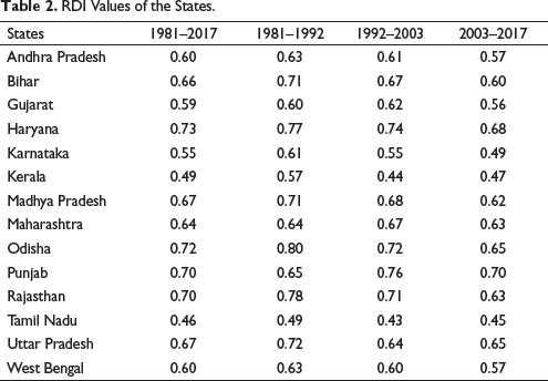
To construct an HHI Index, the total own source revenue (18 taxes) is broadly classified into four categories, that is, taxes on income; taxes on property and capital transactions; taxes on commodities and services; and states’ own non-tax revenue. Based on an inter-temporal analysis of the changing fiscal scenario and implementation of new economic policies and considering the path of fiscal adjustment, the period of the study has been sub-divided into three phases (Table 2).

Table 2.

RDI Values of the States.

States	1981–2017	1981–1992	1992–2003	2003–2017
Andhra Pradesh	0.60	0.63	0.61	0.57
Bihar	0.66	0.71	0.67	0.60
Gujarat	0.59	0.60	0.62	0.56
Haryana	0.73	0.77	0.74	0.68
Karnataka	0.55	0.61	0.55	0.49
Kerala	0.49	0.57	0.44	0.47
Madhya Pradesh	0.67	0.71	0.68	0.62
Maharashtra	0.64	0.64	0.67	0.63
Odisha	0.72	0.80	0.72	0.65
Punjab	0.70	0.65	0.76	0.70
Rajasthan	0.70	0.78	0.71	0.63
Tamil Nadu	0.46	0.49	0.43	0.45
Uttar Pradesh	0.67	0.72	0.64	0.65
West Bengal	0.60	0.63	0.60	0.57

Phase I: From 1981–1982 to 1991–1992 (period with lesser fluctuations in the macroeconomic variables in the economy).

Phase II: From 1992–1993 to 2002–2003 (period marked by fiscal imbalance, fiscal deterioration, characterised by increase in revenue deficit, fiscal deficit and off-budget borrowings).

Phase III: From 2003–2004 to 2016–2017 (period of fiscal improvement, fiscal soundness, characterised by decrease in revenue deficit and increase in tax collection).

For each of the 14 major states of India, Table 2 illustrates the change in the levels of diversification within and across the states over different sub-periods. As per the observation, one of the prominent fiscal trends in the state finances is the gradual decrease in the level of revenue diversification, more so in the recent decades as compared to the 1980s. In the 1980s, the level of diversification was relatively higher across states such as Odisha, Rajasthan, Haryana, Bihar, Madhya Pradesh and Uttar Pradesh. During the first and third sub-periods, a greater number of states fall within 60–80 RDI range and exhibit a higher level of diversification. In the 1990s, due to fiscal deterioration in the state finances, mainly from the mid-1990s, followed by a constant fall of non-tax revenue, besides fluctuations in several major taxes and the preponderance of sales tax in the total taxes, the level of diversification further decreased.

During the post-FRBM period, the extent of diversification showed a progressive trend, but due to several constraints associated with reform measures, revenue collection was not much more progressive and not even consistent during the period of accelerated economic growth (2004–2008). In the late 2000s, followed by an economic recession, lack of consistency in the growth of non-sales tax and more fluctuations in the various components of non-tax revenue further contributed to a lower level of diversification.

Even after the enactment of fiscal reform measures, the states’ attempt to enhance their own revenue generation was not progressive in the long run. As depicted in Table 2, among the 14 states, Haryana, Punjab, Madhya Pradesh and Uttar Pradesh come under a relatively more diversified category. In contrast, Tamil Nadu, Kerala and Karnataka are less diversified states with a greater reliance on sales tax and a continuous fall in non-tax revenue. In terms of state-wise ranking, Haryana recorded consistent progress in RDI ranking, while Punjab, since the 1990s, has witnessed a notable improvement in its RDI ranking. On the contrary, Bihar, Odisha and Rajasthan experienced a constant fall in their RDI rankings, despite being relatively highly diversified states, until the mid-1990s. Finally, no such variability in the HHI values and RDI rankings is noticed in respect of Maharashtra, Andhra Pradesh, Gujarat and West Bengal. In the 1980s, more fiscally stressed states like Odisha, Rajasthan, Bihar, Uttar Pradesh and Madhya Pradesh, excluding Haryana, experienced a more diversified revenue structure. The change in the pattern of diversification, over time, implies that high- and some middle-income states like Punjab, Uttar Pradesh, Karnataka, Kerala and Haryana experienced a relatively progressive trend during the period of fiscal improvement followed by revenue-led reform initiatives in the aftermath of post-reform period. But, in the recent years, mainly in post-recession, a fall in the level of diversification remained much more visible than ever before, in all the states. However, Odisha and Uttar Pradesh are exceptions with a progressive revenue diversification.

Overall, the above analysis reveals that very few states have significantly improved their rankings in RDI, while comparatively many more states have experienced stagnant levels of diversification and some more states have experienced a drastic fall in their RDI rankings.

Theoretical Underpinnings

In the public finance and public choice literature, there are two distinct views with respect to the effect of revenue diversification on the size of government: one is fiscal illusion (revenue complexity) and the other is fiscal stress hypothesis. As per the fiscal illusion hypothesis, there is a systematic misperception of the cost of government on the part of tax payers, and this illusion induces an underestimation of tax prices for public expenditure. Scholars such as Buchanan (1967), Wagner (1976) and Baker (1983) argued that diversifying revenue streams often leads to a ‘fiscal illusion due to increased complexity of tax structure and it leads to a bigger government by increasing public expenditure or tax burden’.

On the contrary, fiscal stress hypothesis propagates that revenue diversification ensures continuity of public service by reducing the cost associated with revenue variability, as variability in revenue has an adverse impact on the size of government (Misiolek & Elder, 1988; White, 1983). So, both the approaches use revenue diversification as a mechanism for estimating the extent of fiscal illusion and also as a protective instrument in terms of bearing the cost of revenue volatility (variability), as per White’s argument (1982). Both approaches find a direct relationship between tax diversification and the size of government. This dichotomy creates some problems when it comes to interpreting revenue diversification used in measuring tax complexity as well as revenue stability (Misiolek & Elder, 1988). Oates (1991) also viewed the revenue complexity and revenue diversification as two competing hypotheses. Based on these views, Carroll observes that revenue complexity does not directly lead to revenue diversification, but revenue diversification results in revenue complexity. While revenue diversification is considered from the point of view of revenue variability or volatility, diversified revenue structures are used as a protective mechanism to control variability in the generation of revenue.

Review of Empirical Studies

The empirical studies provide an overview of different aspects of revenue diversification. Some of the empirical studies discussed below dwell on the different aspects of revenue diversification, considering the economic relationship between revenue diversification and revenue volatility. Until the 1980s, a relatively less attention was placed on the role of revenue diversification in the revenue portfolio. Later, with the initial works of Suyderhoud (1994), the diversification index came to be widely employed in the analysis of revenue structure. As Yan (2008) observed, revenue diversification is a highly desirable goal for the governments due to two reasons. First, it minimizes the loss of revenues during times of severe fiscal crisis and secondly, it even helps governments raise revenue through multiple tax sources during periods of recession. In 2004, Shamsub and Akoto (2004) investigated how state and local governments’ fiscal structures influenced their fiscal performance. Employing a pooled panel approach to the 49 US states-local data for the period of 1982–1997, researchers concluded that local revenue diversification lowered fiscal stress and enhanced their fiscal performance. While examining the role of revenue diversification in reducing revenue instability (volatility), several studies, such as Yan (2008), Carroll and Johnson (2010) and Schunk and Porca (2005), found a negative relationship, in that a diversified revenue structure helped reduce revenue instability with a stable economic base. Likewise, Jimenez and Afonso (2022) assessed the role of tax and non-tax revenue diversification on budgetary solvency with reference to 500 cities in the United States from 2006 to 2011. As per the research outcome, cities that had broadened their revenue structure by tapping non-tax revenue sources were able to handle higher current operational spending with bigger reserves. Revenue-stabilization effects of home rule was examined by Zhang and Nguyen-Hoang (2021). As per the study, increased reliance of home rule cities on property tax to raise more revenue was the major factor behind revenue stability. In contrast, Shi and Jie (2018) found that a diversified revenue structure had an adverse impact on the tax burden, mainly during the economic downturn. The findings suggest that non-tax revenue may help reduce such a burden on taxation. But, Seeun (2013) found a positive association between revenue growth and revenue diversification while noticing the failure of a diversified revenue structure in smoothing revenue volatility. Way back in 1997, Dye and McGuire (1997) had also noticed an adverse impact of revenue diversification on the tax growth rates among the US states.

Some studies have even tried to examine the role of select indirect taxes in reducing revenue variability. While examining the role of a diversified tax structure in the stabilisation of revenue structure, Ebeke and Ehrhart (2011) observed how the implementation of VAT had enhanced tax stability, using panel data of 103 developing countries for the period of 1980–2008. As per the outcome, VAT worked as an instrument of risk diversification besides being less sensitive to economic shocks as compared to the countries that had not implemented it. In contrast, a study by Whitney (2013), for the period of 1983–2004, found how the increased reliance of 35 US states on local option sales tax, with a reduced dependency on property tax, had contributed to revenue volatility.

Going by the existing literature, revenue diversification helps reduce the fiscal stress. However, there is a view that a diversified revenue structure may fail to achieve tax policy goals like efficiency, equity and adequacy (Ladd & Dana, 1987), and in addition, it may lead to expenditure inefficiency and a higher tax burden (Wagner, 1976) on the part of governments.

On this backdrop, it is essential to empirically test the determinants of revenue diversification in the following section.

Determinants of Revenue Diversification

After having observed the pattern and extent of revenue diversification, it is important to study the factors determining such diversification. Regarding the choice of variables, this study has adopted the methodology approach of Purohit and Purohit (2009). The variables and their data sources considered in the model are presented in Table A1 in Appendix A.

As tax and non-tax revenue sources are accounted for in the process of constructing a diversification index, the sub-categories of GSDP, such as the respective shares of service, construction and real estate, mining, and the area under food grains in the total cropped area (the contribution of agriculture), are used as the base for tax revenue. In order to account for the contribution of non-tax revenue, the major contributors of non-tax revenue sources such as education, health, road, water supply and sanitation and major and minor irrigation are used. Following the literature, urbanisation, schools, teachers (education), irrigated area, urban density (water supply and sanitation) and agriculture GSDP (major and minor irrigation) are used as proxies for the above five services. To account for the influence of non-economic factors (political and structural dummies), the study has further employed step and pulse dummies in the analysis.

Empirical Framework and Results

The methodology used in the present analysis is the dynamic panel model. The CD-test (Pesaran, 2004, 2015) is used to test the cross-sectional dependence (CSD) of the variables, which is robust to non-stationarity, parameter heterogeneity and structural breaks.

{CSD}_{Pesaran} = \frac{\sqrt{2 T}}{N (N - 1)} (\sum_{i = 1}^{N - 1}) \sum_{j = i + 1}^{N} \hat{ρ l j}) N (0, 1) .

Since CSD exists (Table 3), second generational unit root tests have been employed as they assume the existence of CSD errors. While working on the large panel, following the results of the CSD, testing the unit root is common to finding the existence of a spurious correlation and to detect the order of integration of each variable. The second generational unit root test CADF is described as follows:

Δ y_{i, t} = α_{i} + β_{i} y_{i, t - 1} + γ_{i} {\bar{y}}_{t - 1} + δ_{i} Δ {\bar{y}}_{t} + φ Δ {\bar{y}}_{t - 1} + u_{i, t,} u_{it} = λ_{i} f_{t} + ε_{i, t .}

Table 3.

Pesaran CD-Test.

Variables	CD	P value
Log per capita GSDP	52.5	0.000***
Revenue diversification	14.51	0.000***
SST GSDP – Share of service GSDP\total GSDP	44.76	0.000***
STT GSDP – Share of transport GSDP\total GSDP	51.68	0.000***
SMT GSDP – Share of mining GSDP\total GSDP	3.007	0.000**
SPS GSDP – Share of primary sector\total GSDP	15.59	0.000***
SCT GSDP &UD – Share of construction and real estate GSDP in the total gross state domestic product and urban density	39.18	0.000***
Irrigation – percentage of gross cropped area irrigated	30.72	0.000***
Foodgrains – Share of area under food grains in the gross cropped area	24.98	0.000***
Number of schools	33.71	0.000***
Log of urban density	3.905	0.000***
STT GSDP – Share of construction and real estate GSDP\total GSDP	15.54	0.000***

Note: *** Denotes significant at 1% level.

where $\bar{y} = N^{- 1}$ $\sum_{j = 1}^{N} y$ _jt, ∇ $\bar{y}$ _t = $N^{- 1} \sum_{j = 1}^{N} Δ y$ _jt.

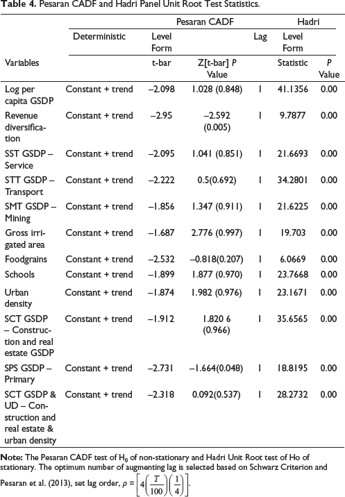
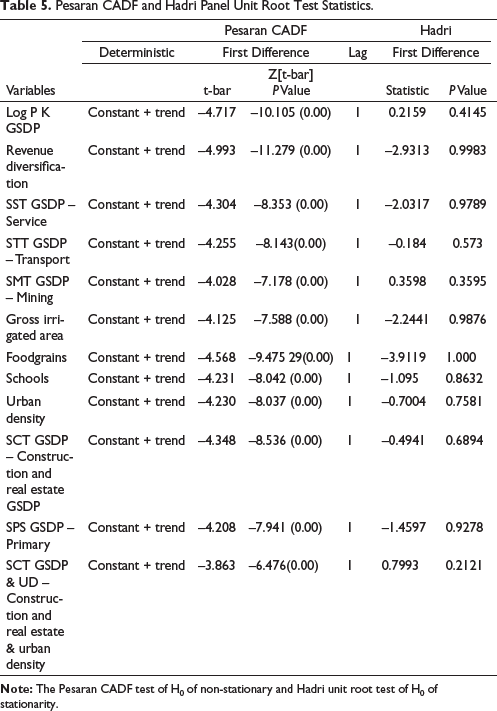
The above equation is augmented with the CSA of the lagged levels and the first differences of the variable. $\bar{y}$ _t-1 is the mean of lagged levels, ∇ $Δ \bar{y}$ _t is the mean of the first differences, and ∇ $Δ \bar{y}$ _t-1 is used to remove time series dependence with a larger T. They are used as proxies for unobserved single common factors f_t.

Tables 4 and 5 provide the results of panel unit root tests. The results are found to be mixed in respect of a few variables at level. As per the CADF panel unit root test, except for revenue diversification, the remaining variables are non-stationary at level. But as per Hadri and Berting test statistics, all the variables are non-stationary at level. Overall, as per the results, all the variables are stationary at the first difference, and no variable is integrated with order two, I(2).

Table 4.

Pesaran CADF and Hadri Panel Unit Root Test Statistics.

		Pesaran CADF			Hadri
	Deterministic	Level Form		Lag	Level Form
Variables		t-bar	Z[t-bar] P Value		Statistic	P Value
Log per capita GSDP	Constant + trend	–2.098	1.028 (0.848)	1	41.1356	0.00
Revenue diversification	Constant + trend	–2.95	–2.592 (0.005)	1	9.7877	0.00
SST GSDP – Service	Constant + trend	–2.095	1.041 (0.851)	1	21.6693	0.00
STT GSDP – Transport	Constant + trend	–2.222	0.5(0.692)	1	34.2801	0.00
SMT GSDP – Mining	Constant + trend	–1.856	1.347 (0.911)	1	21.6225	0.00
Gross irrigated area	Constant + trend	–1.687	2.776 (0.997)	1	19.703	0.00
Foodgrains	Constant + trend	–2.532	–0.818(0.207)	1	6.0669	0.00
Schools	Constant + trend	–1.899	1.877 (0.970)	1	23.7668	0.00
Urban density	Constant + trend	–1.874	1.982 (0.976)	1	23.1671	0.00
SCT GSDP – Construction and real estate GSDP	Constant + trend	–1.912	1.820 6 (0.966)	1	35.6565	0.00
SPS GSDP – Primary	Constant + trend	–2.731	–1.664(0.048)	1	18.8195	0.00
SCT GSDP & UD – Construction and real estate & urban density	Constant + trend	–2.318	0.092(0.537)	1	28.2732	0.00

Note: The Pesaran CADF test of H₀ of non-stationary and Hadri Unit Root test of Ho of stationary. The optimum number of augmenting lag is selected based on Schwarz Criterion and Pesaran et al. (2013), set lag order, ρ = $[4 (\frac{T}{100}) (\frac{1}{4})$ .

Table 5.

Pesaran CADF and Hadri Panel Unit Root Test Statistics.

		Pesaran CADF			Hadri
	Deterministic	First Difference		Lag	First Difference
Variables		t-bar	Z[t-bar] P Value		Statistic	P Value
Log P K GSDP	Constant + trend	–4.717	–10.105 (0.00)	1	0.2159	0.4145
Revenue diversification	Constant + trend	–4.993	–11.279 (0.00)	1	–2.9313	0.9983
SST GSDP – Service	Constant + trend	–4.304	–8.353 (0.00)	1	–2.0317	0.9789
STT GSDP – Transport	Constant + trend	–4.255	–8.143(0.00)	1	–0.184	0.573
SMT GSDP – Mining	Constant + trend	–4.028	–7.178 (0.00)	1	0.3598	0.3595
Gross irrigated area	Constant + trend	–4.125	–7.588 (0.00)	1	–2.2441	0.9876
Foodgrains	Constant + trend	–4.568	–9.475 29(0.00)	1	–3.9119	1.000
Schools	Constant + trend	–4.231	–8.042 (0.00)	1	–1.095	0.8632
Urban density	Constant + trend	–4.230	–8.037 (0.00)	1	–0.7004	0.7581
SCT GSDP – Construction and real estate GSDP	Constant + trend	–4.348	–8.536 (0.00)	1	–0.4941	0.6894
SPS GSDP – Primary	Constant + trend	–4.208	–7.941 (0.00)	1	–1.4597	0.9278
SCT GSDP & UD – Construction and real estate & urban density	Constant + trend	–3.863	–6.476(0.00)	1	0.7993	0.2121

Note: The Pesaran CADF test of H₀ of non-stationary and Hadri unit root test of H₀ of stationarity.

Based on the above results, among the dynamic models, the auto-regressive distributed lag model and CS-ARDL (Pesaran et al., 1999, 2015) are a more preferable approach when the variables are integrated with mixed order I(1) & I(0), and no variable is integrated with order two, I(2).

The CS-ARDL model is as follows:

Y_{i, t} = \sum_{k = 1}^{p} φ_{i, k} y_{i, t - k} + \sum_{l = 0}^{q} β_{i, 1}^{'} x_{i, t - 1} + \sum_{l = 0}^{\bar{z}} ψ_{il}^{_{'}} {\bar{Z}}_{t - 1} + u_{i, t} .

where φi = − (1 − ρ_il) is the speed of adjustment parameter and is expected to be negative and significant. β₁X_1it is the vector of all explanatory variables, and $\bar{z}$ _t = ( $\bar{y}$ _t, $\bar{, x}'$ _t) is the cross-section average of variables.

Before moving on to the CS-ARDL model, to check whether the non-stationary I(1) economic variables are co-integrated, the Pedroni and Westerlund (Westerlund, 2007) co-integration methods are employed to test the null hypothesis of no co-integration (several quantitative variables are stationary at first difference). Pedroni’s (1995, 1999, 2004) residual-based test statistics are based on the assumption that all the variables are integrated at I(1), which assumes both intercept and slope heterogeneity. Out of seven statistics, four are based on pooling data in the within-dimension (panel co-integration), and the remaining three are averaging values for each unit in the between-dimension (group mean co-integration). Residuals extracted from the level and differenced regressions are used in autoregression form to estimate the variance and long-run covariance and to use those to estimate each test statistic (Barbieri, 2009; Pedroni, 1999, 2004).

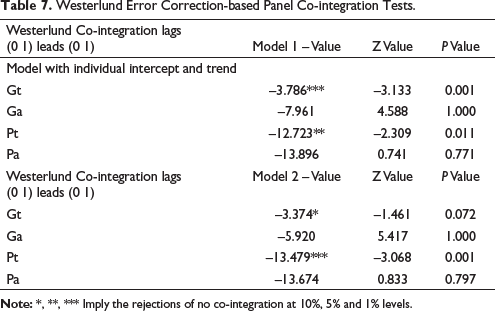
The test results of both the panel and group statistics presented in Table 6 prove the cointegration between the variables. Model 1 includes mining, Model 2 includes the primary sector, and Model 3 includes schools (Table 6). Excluding these three variables, construction and real estate, service, transport, urban density and food grains have been retained in all three models. The test results of Pedroni, supported by the Westerlund co-integration method presented in Table 7, reject the null hypothesis of no co-integration between the variables. Model 1 includes teachers and Model 2 includes area under food grains in the total cropped area (Table 7). Excluding these two variables, construction and real estate, service, transport and irrigation have been retained in the two models.

Table 6.

Pedroni Error Correction-based Panel Co-integration Tests.

Pedroni Co-integration	Model 1	Model 2	Model 3
Model With Individual Intercept and Trend
Panel Statistics
V Statistics	–1.342	–1.252	–1.348
Rho Statistics	0.209	0.2492	0.165
pp Statistics	–6.48***	–6.742***	–7.053***
ADF Statistics	–3.757***	–5.236***	–4.146***
Group Statistics
Rho Statistics	1.507	1.439	1.327
Pp Statistics	–6.509***	–7.012***	–7.315***
ADF Statistics	–4.276***	–5.874***	–3.806***

Note: *** Implies rejection of no co-integration at 1% levels.

Table 7.

Westerlund Error Correction-based Panel Co-integration Tests.

Westerlund Co-integration lags (0 1) leads (0 1)	Model 1 – Value	Z Value	P Value
Model with individual intercept and trend
Gt	–3.786***	–3.133	0.001
Ga	–7.961	4.588	1.000
Pt	–12.723**	–2.309	0.011
Pa	–13.896	0.741	0.771
Westerlund Co-integration lags (0 1) leads (0 1)	Model 2 – Value	Z Value	P Value
Gt	–3.374*	–1.461	0.072
Ga	–5.920	5.417	1.000
Pt	–13.479***	–3.068	0.001
Pa	–13.674	0.833	0.797

Note: *, **, *** Imply the rejections of no co-integration at 10%, 5% and 1% levels.

Following the Pedroni and Westerlund co-integration test results, in order to consider the short- and long-run relationship between variables and also the influence of time-specific dummies that represent the policy as well as non-economic factors in influencing the level of revenue diversification and some of the economic variables that are stationary at level, the ARDL model is employed. ARDL is more preferable, when the variables are integrated with mixed order I(1) and I(0) and no variable is integrated with order two, I(2). The ARDL model assumes heterogeneous slopes in the short run. It helps in analysing the contemporaneous impacts and speed of adjustment to equilibrium and long-run coefficients (slops) are homogeneous, which is more preferable for moderate T compared to the dynamic fixed effect and mean group model. Since N is small, this analysis employs PMG-adjusted for cross-section dependence (PMG is quite robust to outliers and the choice of lag orders; Pesaran & Smith, 1995). The CS-ARDL model is augmented with the lagged cross-section mean of the variable and its lags. The ARDL methodology assumes that errors are independently distributed across t and i. If the unobserved common factor in the error term is correlated with the regressors and the failure to account for dependency, it results in inappropriate standard errors and biases the coefficients (Pesaran, 2006).

Estimation methods: The ARDL model is written as follows:

Y_{j, t} = δ \sum_{k = 1}^{p} φ_{i, k} y_{i, t, - k} + \sum_{l = 0}^{q} {β^{'}}_{i, 1} x_{i, t - 1} + u_{i, t}

Its cointegration form would be

Y_{j, t} = θ_{i, x_{i, t}} + α_{I}^{'} (L) Δ x_{i t} + {\tilde{u}}_{i, t, t} {\tilde{u}}_{i, t} = γ_{i}^{'} F_{t} + ε_{i, t}

where φ_i = − (1 − ρ_il) is the speed of adjustment parameter and it must be non-zero, expected to be negative and significant. It represents bringing the variable back to a long-run equilibrium. The short-run coefficients and the speed of adjustment to the long-run from short-run deviation and error variances differ across units, whereas in the long-run, coefficients are assumed to be homogeneous across units. θ_i = θ,_I, i = 1,2…..,N. θ_i is estimated to find out whether the variables are exogenous or endogenous and are I(0) or I(1) in nature (Pesaran et al., 1999).

θ_{i} = \frac{\sum_{l = 0}^{q} β_{i, 1}}{1 - \sum_{l = 1}^{p} φ_{i, 1}}

where p is the lag of the dependent variable and q is the lag of the independent variable.

To overcome the problem of unobserved common factors, following the seminal work of Chudik et al., (2013), CS-ARDL approach was employed, following the CCE methodology of Pesaran (2006). When the feedback effects from the lagged values of the dependent variable to the independent variables exist, $\tilde{u}$ _it is correlated with x_it, then the distributed lag model would be inconsistent.

The CS-ARDL model is

Y_{i, t} = \sum_{k = 1}^{p} φ_{i, k} y_{i, t - k} + \sum_{l = 0}^{q} β_{i, 1}^{'} x_{i, t - 1} + \sum_{l = 0}^{\bar{z}} ψ_{il}^{_{i}} {\bar{Z}}_{t - 1} + u_{i, t}

where $\bar{z}$ _t = ( $\bar{y}$ _t, $\bar{, x}'$ _t)’ & $\bar{z}$ = $(\frac{1}{3})$ cross-section averages of current and lags of dependent and independent variables. The selection of lag length is crucial. The lag order of 1 is chosen considering the time period and number of explanatory variables used in this analysis.

The test results of the CS-ARDL panel regression models are reported in Table 8. Each table contains different models with different sets of control variables. The empirical analyses, with the inclusion of cross-section averages, successfully account for the presence of common factors across units. The CS-ARDL model helps take care of the potential endogeneity of political variables. Focusing on the long-term coefficients, most of the variables are found to be statistically significant and the EC [yt − 1] refers to the Error-Correction term (speed of adjustment parameter), which is statistically significant at 1% and confirms co-integration in the long run.

Table 8.

Dependent Variable: RDI (CS-ARDL Model).

Explanatory Variables	Model I
Dependent Variable	$R e v e n u e D$ Revenue D iversification
ECT	–0.2908 (–3.08)***
Long Run
SST GSDP – Service	–0.603 (–5.19)***
STT GSDP – Transport	2.696 (5.40)***
Irrigation	6.233 (5.10)***
Schools	2.966 (6.41)***
PM GSDP – Primary	0.438 (5.17)***
Log Urban Density	0.00222 (0.24)
SCT GSDP-C and Real estate	–1.486 (–4.63)***
VAT	–0.0600 (–2.96)***
FRL	0.0134 (0.67)
BLEY	–0.0115 (–2.43)**
LEY	–0.0699 (–6.64)***
Regional parties	–0.0220 (–3.15)***
Coalition governments	–0.0220 (–1.91)*
Incumbency	0.0940 (7.78)***
Short Run
∇SST GSDP – Service	0.266 (0.65)
∇STT GSDP – Transport	0.910 (1.13)
∇SCT GSDP & UD – Construction and real estate & urban density	–0.207 (–0.37)
∇log of Urban Density	–0.0588 (–1.23)
∇ Gross Irrigated Area	5.144 (0.16)
∇Schools	3.911 (0.03)
∇FRL	0.00806 (0.38)
∇RD(-1)	–0.0733 (–0.88)
∇STT GSDP – Transport (–1)	–2.625 (–3.00)***
∇PMGSDP – Primary (–1)	–0.0979 (–0.45)
Constant	0.0536 (2.43)**
N	460
CD-test (p value), corr	–0.63 (0.537), –0.013

Note: ***p < .01, **p < .05, *p < .1 levels of significance, respectively. T-statistics are shown in parentheses. ∇ represents first difference. Period (1981–2015).

In the CS-ARDL model, column 2 of Table 8 indicates that most of the economic variables are significant. Different components of GSDP are the core independent variables used in this model. Among the long-run coefficients, the share of transport GSDP, primary GSDP, the school proxy for education and irrigation are significant and positively associated with revenue diversification, whereas service, construction, and real estate GSDPare are negatively associated with it.

The primary sector of the economy includes agriculture, forestry, fishing, mining and quarrying. As per the regression outcomes, irrigation, which is used as a proxy for agriculture GSDP, is positive and relatively more significant despite overall primary sector GSDP significantly contributing to revenue diversification. This shows the importance of the agricultural sector in widening the tax base in India.

In own tax portfolio, sales tax, excise duties, stamp and registration fees, and motor vehicle taxes have progressively contributed to a higher tax revenue buoyancy. However, among the major tax sources, only sales and excise duties accounted for a larger share of the total own tax revenue till 1997, while a gradual improvement in stamp duties and electricity duties thereafter has contributed positively towards a diversified revenue structure since the mid-2000s but failed to maintain sustained growth for a longer duration in the period of post-recession.

The nature and structure of a revenue portfolio are very much crucial to a diversified revenue structure. Taxes, which are relatively more elastic in nature, show fluctuations with economic ups and downs. Among the major taxes, stamps and registration, and commercial taxes (sales tax) are relatively more elastic as compared to motor vehicle and excise duties. Revenue from sales, a major revenue source, being relatively elastic, shows fluctuations with an economic slowdown. Even revenue from motor vehicle and excise duties shows a decrease with the economic downturn due to a lack of demand-led growth, and several stimulus measures undertaken by the respective state governments and the central governments towards stimulating demand may have further reduced revenue collection in the post-recession period (MTFP, various issues).

In own tax portfolio, only sales tax has been the most buoyant and elastic among all the other taxes for a longer period, negatively contributing to a diversified revenue structure. Furthermore, the implementation of VAT as a step towards tax reform has had an adverse impact on the process of revenue diversification. It is probably because of the greater emphasis placed on sales tax reforms since the last decade on generating more revenue with the implementation of VAT.

In non-tax category, education, health, roads, water supply, sanitation and major and minor irrigation have contributed significantly towards a diversified revenue structure, though it has failed to maintain consistency over a longer period. For instance, in the 1990s, the dismal performance of non-merit services such as irrigation, co-operation and uneconomic transport fares, the poor performance of the state PSUs, huge losses incurred by state electricity boards, and lower recovery rates were evedent fluctuations in general and economic services was evident. The trend got reversed with the states’ constant effort to mobilise additional resources through tax and non-tax sources towards improving the state of the fiscal situation from crisis to stability over the period of 2001–2011. A better recovery of user charges with respect to irrigation in the early 2000s and a relatively progressive contribution of economic, irrigation and mineral resources to non-tax revenue altogether contributed positively to the level of revenue diversification. Although, due to several constraints associated with reform initiatives, diversified revenue collection has not remained much progressive since 2008, following an economic recession, due to a lack of a strategic policy to cope with such economic ups and downs. With such an erratic growth pattern displaced by major non-tax revenue sources, annual growth rates of various components of non-tax revenue have remained more volatile with year-to-year fluctuations across states and time.

Among the components of tax and non-tax revenue, despite progressive growth, sluggishness and wide fluctuations in the growth pattern are more evident. As per the above outcomes, stamps and registration fees, taxes on vehicles, the real estate boom, agricultural taxation and reforms in motor vehicle taxes have contributed positively towards mobilisation of revenue from non-sales taxes (state finances 2008–2009). In addition, the contribution of social and economic services from non-tax revenue, such as major and minor irrigation, education and roads, is positive and significant with respect to the level of revenue diversification. The real estate boom and ongoing urbanization, together representing real estate activities and reforms, mainly in the urban area, are responsible for such an outcome. Nevertheless, a huge unevenness in the amount of revenue collection across the states and over time has had an adverse impact on the level of diversification of the revenue structure.

Among political variables, as per the empirical outcome, excluding ‘incumbency’, election dummies, regional parties and coalition government are negatively significant. This implies that when the arena of politics is competitive and a coalition is in place, governments tend to focus more on pre-poll uneconomic populist programmes/decisions to win elections by showcasing the temporary relief benefits rather than undertaking long-term revenue mobilization initiatives as part of widening the tax base.

The rise of coalition governments and regional parties since 1989 has reduced the dominance of a single party while increasing the trend of political uncertainty. At the same time, regional parties have started to follow their own respective development models to retain power over a longer period. However, political coalitions, with an increase in the number of affiliated political parties coming together with different pre-election agendas and political ideologies, have often failed to mobilize sufficient revenue from a diverse set of sources. As citizens are generally reluctant to pay taxes, ruling parties have failed to prioritise more revenue mobilization from a diverse set of sources.

As people generally dislike paying taxes and the most often political parties show an inclination to move towards a massive reduction in tax rates, unlimited, unscientific ways of tax exemptions and concessions may lead to a massive erosion in tax revenue collection. If the parties in power focus more on identity politics, a lack in the timing of fiscal reforms and long-term strategies towards mobilising resources may further increase the states’ capacity and policy to cope with economic ups and downs, further increasing their continued dependence on a very few revenue sources. The states’ reluctance to raise revenue from a diverse set of sources is also one of the reasons for poor tax buoyancy.

On the contrary, ‘incumbency dummy’ is positive and significant. This implies that when the same party/government is re-elected in the coming elections, it may focus on mobilizing revenue from additional sources. Once re-elected, the ruling party more often faces increased pressure to mobilize sufficient revenue to continue or undertake expenditure obligations, and that may force the government to take initiatives towards widening the tax base.

Overall, it is evident from the analysis that both economic and non-economic variables play a crucial role in the process of revenue structure diversification. States seem to be less enthusiastic about diversified revenue generation from non-tax revenue sources.

Conclusions and Policy Suggestions

The study has explored the extent and changing trends in the level of revenue diversification and subsequently focused on the determinants of such diversification among selected Indian states. A proper diversification of revenue basket serves as an important cushion against any internal or external fiscal shocks associated with the slowdown of economic activities. The present analysis has thrown up some interesting findings as well. Cyclical fluctuations in the major tax sources with a lesser emphasis on non-tax revenue because of non-revision of user charges, non-recovery of user charges, and even poor monitoring of the collection of user charges have had an adverse impact on the process of revenue diversification on the part of states. Overall, the states have failed in their planning in the due course of proper fiscal management initiatives to mobilize adequate revenues. Over the decades, a lack of macroeconomic vision has been observed on the part of states towards diversified revenue generation from different sectors with an overreliance on a few revenue sources.

Governments have to choose between healthy revenue generation and providing a stimulus to the economy through lower prices. Since public services are largely in the nature of economic and social services with a high socio-economic importance attached, there is a need for rationalising the existing user charges in a way that will not affect the demand for public goods such as education and health. This is a matter of concern that needs policymakers’ due attention. If states could diversify their revenue baskets with more non-sales taxes as well as non-tax revenue sources, it is an indication of a higher level of diversification.

Appendix A

Table A1.

Variable Specifications and Data Sources.

Variables	Definition and Data Sources
RDI (Revenue Diversification)	HHI Values
Share of Service GSDP\Total GSDP	National Accounts Statistics
Share of Transport GSDP\Total GSDP	–
Share of Construction and Real Estate GSDP in the Total GSDP and Urban Density	–
Share of Primary Sector GSDP/Total GSDP	–
Share of Mining/Total GSDP	–
Irrigation, measured as a percentage of gross cropped area irrigated	Directorate of Economics and Statistics, MOA
Number of schools	Selected Educational Statistics
VAT (value-added tax) – One of the institutional reforms introduced by state governments in 2005. It is used as a dummy variable to capture its impact on revenue diversification, as it is a major policy change.	State Finance Documents
FRBM (Fiscal Responsibility and Budget Management Act) – One of the institutional reforms initiated by state governments enacted in 2003	–
Form of government-coalition or single party is in power at the state level (takes value 1 if the coalition government is in power, 0 otherwise).	Election Commission of India
Political incumbency takes value 1 if there is change in the ruling party in the next state legislative assembly, 0 otherwise.	–
Regional party takes value 1 if the regional party is in power, 0 otherwise.	–
Electoral cycle dummies (ELA) – election year of state legislative assembly; BELA – 1 year prior to election.	–
Urban Density	Census of India

Footnotes

Declaration of Conflicting Interests

The authors declared no potential conflicts of interest with respect to the research, authorship and/or publication of this article.

Funding

The authors received no financial support for the research, authorship and/or publication of this article.

ORCID iD

J.S. Darshini

References

Baker

S. H.

(1983). The determinants of median voter tax liability: An empirical test of the fiscal illusion hypothesis. Public Finance Quarterly , 11(1), 95–108.

Buchanan

J. M.

(1967). Public finance in a democratic process . Chapel Hill: University of North Carolina Press.

Carroll

D. A.

& Johnson

(2010). Examining small town revenues: To what extent are they diversified? Public Administration Review , 70(2), 223–253.

Chakraborty

(2014). Fiscal reforms, fiscal rule and development spending: Two decades of Indian experience. In R. Khasnabis & I. Chakraborty (Eds.), Market, regulations and finance: Global meltdown and the Indian economy (1st ed., pp. 1–26). Springer. Retrieved from https://www.researchgate.net/publication/299748905

Chudik

, Mohaddes

, Pesaran

M. H.

, & Raissi

(2013). Debt, inflation and growth: Robust estimation of long-run effects in dynamic panel data models . (Globalization Institute Working Papers 162). Federal Reserve Bank of Dallas.

Dye

R. F.

, & McGuire

T. J.

(1997). The effect of property tax limitation measures on local government fiscal behaviour. Journal of Public Economics , 66(3), 469–487.

Ebeke

C. H.

, & Ehrhart

(2011). Is vat stabilizing? CERDI. Retrieved from https://halshs.archives-ouvertes.fr/halshs-00617272v1

Ebeke

, & Ehrhart

(2013). Tax revenue instability in sub-saharan Africa: Consequences and remedies, Journal of African Economies , 21(1), 1–27.

Hadri

(2000). Testing for unit roots in heterogeneous panel data. Econometrics Journal , 3(2), 148–161.

10.

Jimenez

B. S.

, & Afonso

W. B.

(2022). Revisiting the theory of revenue diversification: Insights from an empirical analysis of municipal budgetary solvency. Public Budgeting & Finance , 42(2), 196–220. Retrieved from DOI: 10.1111/pbaf.12309.

11.

Kurian

J. N.

, & Sushmita

(2004). Rising revenue gap of the states – dimensions of the problem and possible approaches for a solution . New Delhi: NIPFP. Retrieved from, https://fincomindia.nic.in/

12.

Ladd

H. F.

& Dana

R. W.

(1987). State and local tax systems: Balance among taxes vs. balance among policy goals. In Stocker

Frederick D.

(ed.), The quest for balance in state-local revenue structures (pp. 39–69). Tax Policy Roundtable/Property Tax Papers Series TPR-16, MA: Lincoln Institute of Land Policy.

13.

Purohit

M. C.

, & Purohit

V. K.

(2009). Mobilising non-tax revenue: An empirical analysis of trends in states. Economic and Political Weekly , 44(5), 54–62.

14.

Medium term fiscal plan for Karnataka - 2002 to 2018, various issues.

15.

Misiolek

W. S.

& Elder

H. W.

(1988). Tax structure and the size of government: An empirical analysis of the fiscal illusion and fiscal stress arguments. Public Choice , 57(3), 233–245.

16.

Mukherjee

(2019). State of public finance and fiscal management in India during 2001-16 (Working Paper 265). New Delhi: NIPFP.

17.

Oates

W. E.

(1985). Searching for Leviathan: Empirical study. American Economic Review , 75, 748–757.

18.

Oates

W. E.

(1991). On the nature and measurement of fiscal illusion: A survey. Retrieved from: http://psu.edu

19.

Pedroni

(1995). Panel cointegration; asymptotic and finite sample properties of pooled time series tests, with an application to the PPP hypothesis (Working Paper 92−013). Indiana University.

20.

Pedroni

(1999). Purchasing power parity tests in co-integrated panels (Working Paper 1−5). Indiana University.

21.

Pedroni

(2004). Panel cointegration: Asymptotic and finite sample properties of pooled time series tests with an application to the PPP hypothesis. Econometric Theory , 20, 597–625.

22.

Pesaran

M. H.

, Shin

, & Smith

R. P.

(1999). Pooled mean group estimation of dynamic heterogeneous panels. Journal of the American Statistical Association , 94(446), 621–634.

23.

Pesaran

M. H.

, & Smith

(1995). Estimating long-run relationships from dynamic heterogeneous panel. Journal of Econometrics , 68(1), 79–113.

24.

Pesaran

M. H.

(2006). Estimation and inference in large heterogeneous panels with a multifactor error structure. Econometrica , 74(4), 967–1012.

25.

Pesaran

M. H.

(2015). Testing weak cross-sectional dependence in large panels. Econometric Reviews , 34, 1089–1117.

26.

Pesaran

M. H.

, Smith

L. V.

, & Yamagata

(2013). Panel unit root tests in the presence of a multifactor error structure. Journal of Econometrics , 175(2), 94–115.

27.

Rajaraman

(2004). Fiscal development and outlook in India (Working Paper 04/15). New Delhi: NIPFP.

28.

Rathin

(2022). Changing fiscal dynamics . Retrieved from https://www.india-seminar.com/2019/717/717_rathin_roy.htm

29.

Reserve Bank of India, State Finances A Study of Budgets of 2008-09 to 2015-16.

30.

Schunk

, & Porca

(2005). State-local revenue diversification, stability and growth: Time series evidence. Review of Regional Studies , 35(3), 246–265.

31.

Seeun

(2013). Revenue strategies of US states under conditions of economic and political stress: Revenues diversification 1980 to 2011 . [ASU Electronic Theses and Dissertation]. Arizona State University.

32.

Shamsub

, & Akoto

J. B.

(2004). State and local fiscal structures and fiscal stress. Journal of Public Budgeting, Accounting & Financial Management , 16(1), 40–61.

33.

Shi

, & Jie

(2018). “Faulty” fiscal illusion: Examining the relationship between revenue diversification and tax burden in major U.S. cities across the economic cycle. Local Government Studies , 44(3), 1–33.

34.

Singh

(2006). State finances in India: A case for systemic reform . (Working Paper 1–37). Retrieved from: http://escholarship.org/uc/item/8560h76z

35.

Suyderhoud

J. P.

(1994). State-local revenue diversification, balance, and fiscal performance. Public Finance Quarterly , 22(2), 168–195.

36.

Wagner

R. E.

(1976). Revenue structure, fiscal illusion, and budgetary choice. Public Choice , 29(1), 127–132.

37.

Westerlund

(2007). Testing for error correction in panel data. Oxford Bulletin of Economics and Statistics , 69(6), 709–748.

38.

White

F. C.

(1983). Trade-off in growth and stability in state taxes. National Tax Journal , 36(1), 103–114.

39.

Whitney

B. A.

(2013). Diversification toward stability? The effect of local sales taxes on own source revenue. Journal of Public Budgeting, Accounting & Financial Management , 25(4), 649–674.

40.

Yan

(2008). The impact of revenue diversification and economic base on revenue stability: An empirical analysis of county and state governments. [Doctoral Dissertations]. University Of Kentucky . Retrieved from https://Uknowledge.Uky.Edu/Gradschool_Diss/619

41.

Zhang

, & Nguyen-Hoang

(2021). Home rule and municipal revenue stability: New evidence from Texas. Public Budgeting and Finance , 1–23.