Flyable Tracking of Non-flyable Miss Approach Dubins Trajectories

Abstract

To adequately manage the growing demand for air mobility services, air traffic control systems must increase the density of aircraft in air space, which necessarily implies reducing the separation among them. This work deals with the use of runway approach procedures based on Dubins trajectories, as well as their 4D tracking by aircraft. A method is proposed to define a fictitious aircraft that will describe Dubins trajectories generating a 4D reference, and two tracking mechanisms (basic and improved) following this reference, which can be used by real (flyable) aircraft. These mechanisms have been evaluated in the Málaga airport (Spain), which has a high traffic density during the seasonal period. Simulation results verify their correct operation and high tracking accuracy.

Keywords

Aircraft precision approach navigation error dubins path flyable trajectories dynamic systems differential equations

1. Introduction

According to the International Civil Aviation Organization (ICAO), global air traffic has progressively grown from 1.63 billion passengers in 2002 to 4.56 billion in 2019 Bureau (2020). Although in 2020 the COVID19 pandemic reduced this figure to 2004 levels, once it will be overcome, a rapid recovery of the sector is expected. To adequately manage the growing demand for air mobility services, air traffic control (ATC) systems must increase the density of aircraft in air space, which necessarily implies reducing the separation among them. One way to achieve this is by the use of 4D (3D plus time) trajectory-based operations (De Jong et al., 2011; Enea & Porretta, 2012; Guan et al., 2016, 2017; Klooster et al., 2008; Núñez et al., 2017; Pleter et al., 2009), in which aircraft must be able to move along pre-established routes with high accuracy, keeping the tracking error below a threshold considered unacceptable. Throughout the history of aviation, the complexity of flight routes, as well as the accuracy of their tracking, has progressively improved as technological advances have made it possible. Currently, new airspace concepts support extremely precise manoeuvers, even coordinated among several aircraft ((2016), ICAO).

In this work, we address the problem of aircraft guidance during the final approach flight phase. Starting with the definition of an approach maneuver based on Dubins curves (Dubins, 1957), a fictitious aircraft, acting as a 4D reference, traverses this trajectory with a non-flyable behaviour. On the other hand, the real aircraft, constrained to follow a flyable trajectory with progressive variations of the radius of curvature, employs an autopilot that tracks the aforementioned reference. The autopilot adjusts the aircraft’s heading and speed to reduce the tracking error. To assess our proposals, we have developed a simulator (implemented in MATLAB/Simulink) modelling the runway approach manoeuvre, the autopilot system, and the aircraft dynamics.

The rest of the manuscript is structured as follows. Section 2 Background on Aircraft Navigation describes advances in instrument navigation systems and decomposes the 4D trajectory tracking error in function of its causes. Section 3 Mathematical Modelling elaborates on the dynamics and behavior of a Dubins aircraft, defines an approach procedure as a series of consecutive waypoints, and explores the dynamics and two potential behaviours for a flyable aircraft tracking the Dubins trajectory. Section 4 Performance Evaluation encompasses the performance evaluation of the two proposed autopilot systems. Initially, runway RWY13 of Málaga (Spain) airport is defined. Subsequently, the simulator is described, followed by presentation and analysis of the simulation results. Section 5 Conclusions summarises our overall findings and outlines potential future research works.

2. Background on Aircraft Navigation

Air navigation may be defined as the process of determining the geographic position and maintaining the desired orientation of an aircraft relative to the Earth’s surface. In its early stages, aerial navigation relied primarily on visual references, offering limited possibilities. The incorporation of a compass on board allowed pilots to ascertain the aircraft’s heading (the angle between the longitudinal axis of the aircraft and the magnetic north). This innovation facilitated the adoption of a more sophisticated navigation technique known as ”dead reckoning”, wherein the aircraft’s position could be determined starting from a known position and direction and then proceeding at a specific speed for a defined duration.

2.1. Conventional Navigation

Subsequently, what it is now referred to as conventional instrument-based navigation became reliant on ground-based navigation aids, typically VOR (VHF Omnidirectional Radio Range) transmitters. Aircraft have the capability to determine the angle of the VOR signals they receive, enabling them to navigate along preestablished routes (airways) comprised of multiple legs involving a sequence of ground-based navigation aids (either to or from these ground stations). For instance, Figure 1 illustrates a scenario where an aircraft travels from an origin $(O)$ to a destination $(D)$ utilizing a route consisting of 4 segments. Initially, the aircraft progresses towards the initial radio beacon while maintaining an angle $V_{1} (α)$ with respect to it (aided by an onboard instrument known as Flight Director, which typically assists the pilot in adhering to the desired heading). Upon passing over the beacon, the aircraft veers away while maintaining a departure angle $V_{1} (β)$ . During this divergence, the pilot observes the changing relative angle to the second beacon. When the desired angle $V_{2} (α)$ is reached, then the aircraft leaves that course and repeats the whole process for the next radio beacon. Conventional navigation ensures high precision in the proximity of radio beacons but experiences a decline in accuracy as the distance increases. Conversely, the way in which turns occur is not clearly defined, inducing errors in navigation during segment transition. In conclusion, the navigation is not highly accurate in any part of the route.

Figure 1.

Conventional navigation.

2.2. Area Navigation (RNAV)

The later inclusion, among other systems, of DME (Distance Measuring Equipment) allowed a transition to area navigation (RNAV), a revolutionary method in which aircraft operate on any desired flight path. In this environment, a route is composed of a sequence of abstract waypoints (not necessarily correlated with ground VOR/DME transmitters). The aircraft heads to the waypoint by triangulating the information it obtains from various ground beacons and with RNAV, navigation increases in flexibility, taking on a vital role in ATM efficiency whilst also sustaining safety performance. Figure 2 shows the same example of Figure 1 where the aircraft follows a desired route, defined by 4 waypoints, independent of the 2 radio beacons. The different types of RNAV operations are RNAV 1, RNAV 2, RNAV 5, and RNAV 10. The number indicated in the name refers to the permissible navigation error (as described in the subsection 2.5 Aircraft navigation error).

Figure 2.

RNAV navigation.

2.3. Required Navigation Performance (RNP)

Although RNAV was a considerable improvement in the definition of trajectories followed by aircraft, it does not establish any restriction to the permissible error in their tracking. Moreover, it does not solve the problem of transit from one waypoint to the next, which implies a change of course. Two possibilities are envisaged, on the one hand, a fly-by waypoint will be one where the pilot is required to use turn anticipation to avoid overshoot of the next flight segment. On the other hand, a fly-over waypoint postpones any turn until the waypoint is overflown, and then, the pilot should perform an intercept maneuver of the next flight segment. In any case, the trajectory of the turn is not defined, forcing the pilot to improvise on the fly. This methodology is unacceptable in scenarios with congested airspaces and reduced separation minima among aircraft. Required Navigation Performance (RNP) ((2009), ICAO) is a new methodology that aims to eliminate the previous problem. One of the key differences is that the navigation specifications incorporate on-board performance monitoring and alerting requirements. In addition, RNP explicitly contemplates segments in the form of a circumferential arc (RF, radius to fix legs), indicating to the pilot the exact way to make a course change between consecutive waypoints. Figure 3 shows the same example of previous figures where the aircraft follows a delimited route including straight and curvilinear sections. The most important RNP specifications are RNP 1, RNP 4, Advanced RNP, RNP AR APCH (for approach procedures with vertical guidance), and RNP 0.3 (for helicopters).

Figure 3.

RNP navigation.

2.4. Performance-based Navigation (PBN)

Historically, the waypoints contained in the RNAV and RNP specifications have been defined in terms of the sensors used to locate them (VOR/DME systems, GNSS $\dots$ ), as well as the instrumentation required on board for their correct tracking. This generates a lot of inconveniences. For example, changing the location of a terrestrial radio beacon would imply changing all the specifications that rely on it. On the other hand, existing specifications cannot benefit from further technological developments in navigation instruments. To solve this situation, ICAO developed the concept of performance-based navigation (PBN), in which RNAV and RNP requirements for particular airspace are defined in terms of accuracy, completeness, readiness, continuity, and functionality for the proposed operations. On the basis of these generic specifications, airlines will choose, from the available options, the underlying navigation infrastructure and flight crew procedures that best suit their business interests. An exhaustive review providing background on aircraft PBN systems and supporting technologies can be found in López-Lago et al. (2020).

2.5. Aircraft Navigation Error

Figure 4(a) shows the various contributions to navigation error for an aircraft following a $3 D$ route (for simplicity, vertical tracking error is omitted). Given a desired navigation path, it should be implemented through a sequence of waypoints, assuming a certain path definition error (PDE), perpendicular to the route at each point. In the same way, the distance between the aircraft estimated position and the defined path is called a flight technical error (FTE). On the other hand, the error between the aircraft actual and estimated positions could be decomposed in its longitudinal and lateral components (with respect to the route), named along track error (ATE) and navigation system error (NSE) respectively. Finally, the total system error (TSE) is the sum of the previously defined errors. Figure 4(b) shows navigation error tracking $4 D$ routes, defined as $3 D$ routes including time. On this occasion, the aircraft desired position on the desired path at any given time is explicitly indicated. PDE, FTE and NSE are no longer distances perpendicular to the route and become vectors on the plane. The aim of this work is to minimise the value of FTE when an aircraft executes a flyable actual path following a non-flyable defined path. Consequently, in our simulations, we will assume that the contributions of PDE and NSE are negligible. PDE could be negligible if strict navigation data base integrity processes are performed. NSE could be negligible if accurate navigation systems are employed.

Figure 4.

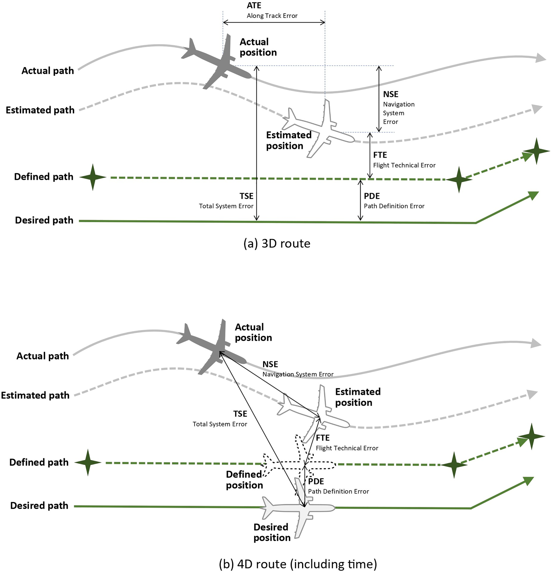
Aircraft navigation error.

3. Mathematical Modelling

First, we will establish the airspace frame and the waypoint-based navigation procedure we assume autopilots follow. Then, we will describe the model for Dubins (reference) and flyable (real) aircraft and three different autopilots. The general relationship among all these components is shown in Figure 5. A preliminary version of some of these models can be found in Casado et al. (2021)

Figure 5.

Overall relationship among mathematical models.

3.1. Airspace Definition

We present the coordinate transformation from the navigation frame to a local tangent frame, which is essential for the path-following strategy employed in this study. In our assumptions, we consider the Earth’s surface to be flat, allowing us to represent the airspace using three vectors $X, Y, Z$ , pointing towards East, North, and upwards, respectively. The origin of coordinates on the horizontal plane is defined at the point of contact between the aircraft and the runway (the touchdown point). On the vertical axis, the origin is set at sea level. A three-dimensional position is denoted as a vector $p = [x y z] \in R^{3}$ , relative to the origin of coordinates. For the sake of simplicity, when the altitude is irrelevant, we work within a two-dimensional plane, redefining the position as $p = [x y] \in R^{2}$ . An orientation $ψ$ in the plane is defined as the angle from North to the aircraft’s orientation, with positive values denoting clockwise rotation. In this context, we define the aircraft’s heading by the orientation of its longitudinal axis.

In summary, the position and heading of an aircraft at a given moment are expressed by its pose $x = [p ψ]$ . For the purpose of our study, the rotation of the aircraft with respect to its axes, typically referred to as roll, pitch, and yaw angles, is deemed irrelevant. Figure 6 provides an illustrative example of an aircraft’s location.

Figure 6.

3D airspace model.

3.2. Dubins-based Aircraft Approach Procedures

Dubins curves (Dubins, 1957) are a mathematical tool widely used in the definition of aircraft and unmanned aerial vehicle trajectories (Chen et al., 2023; Haghighi et al., 2022; Lin & Saripalli, 2014). The Dubins problem consists of finding the shortest connection between two points in a plane while maintaining a restriction on the curvature. A Dubins trajectory is a sequence of segments, in which each of them can be rectilinear or an arc with preestablished constant radius. There cannot be two consecutive rectilinear segments in the sequence, with straight lines and curves usually alternating.

As described in Section Background on Aircraft Navigation, RNP procedures may naturally contain curved segments, but RNAV procedures do not. However, it is possible for an RNAV procedure to conform to a Dubins trajectory, if we calculate the exact point at which the aircraft must transit from the curved fly-by waypoint to the next waypoint in the sequence. Figure 7 shows an example of RNAV procedure defined for a sequence ${w_{1}, w_{2}, \dots, w_{(n - 2)}, w_{(n - 1)}, w_{n}}$ . A waypoint is defined as a vector $w = [p s]$ , where $p \in R^{3}$ establishes its position, and $s \in S$ is the expected fly-over speed.

Figure 7.

RNAV approach executed as a Dubins trajectory.

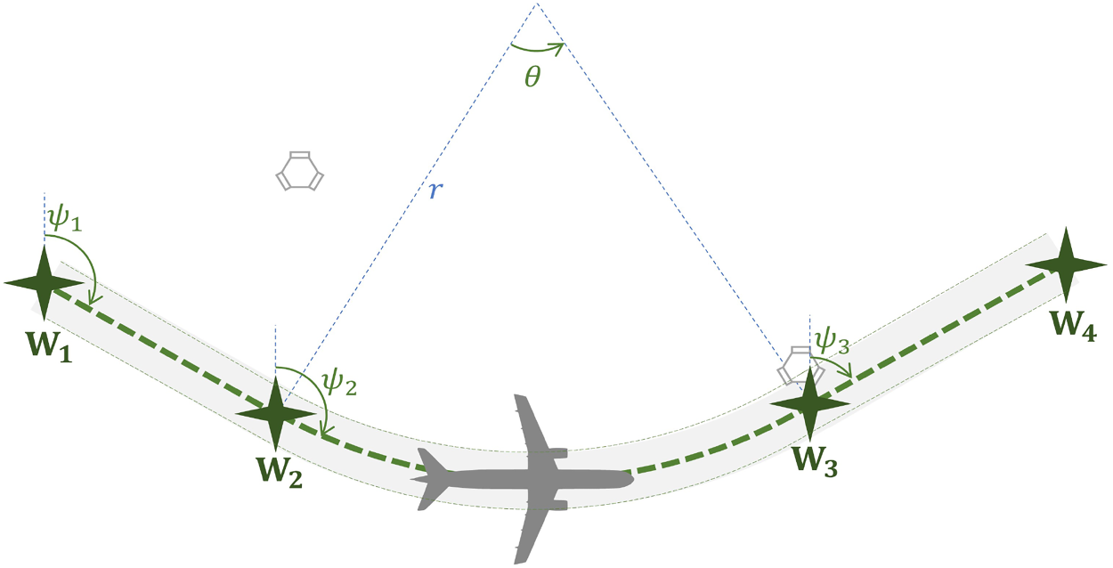
In our proposal, transit points between waypoints are computed as illustrated in Figure 8. Assuming the waypoints sequence ${w_{1}, w_{2}, w_{3}}$ , aircraft a should transit from $w_{2}$ to $w_{3}$ when it is located at position $v_{2} \in R^{2}$ , at a distance d from $w_{2}$ that allows to face $w_{3}$ employing a circular arc of radius $r$ . Table 1 details the algorithm. Planar locations of the waypoints involved in the turn manoeuvre are extracted ( $01 - 02$ ). After that, two unitary vectors among the three waypoints are computed $(03 - 04)$ . Then, the angle between these vectors is obtained, by using the definition of vector dot product (05). This is the turning angle. With it, we obtain distance d (06) and, finally, the position at which the aircraft must start the manoeuvre (07).

Figure 8.

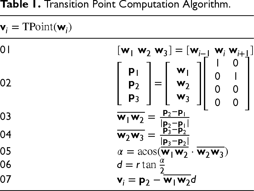
Transition point computation.

Table 1.

Transition Point Computation Algorithm.

$v_{i} = TPoint (w_{i})$
01	$[w_{1} w_{2} w_{3}] = [w_{i - 1} w_{i} w_{i + 1}]$
02	$[\begin{array}{l} p_{1} \\ p_{2} \\ p_{3} \end{array}] = [\begin{array}{l} w_{1} \\ w_{2} \\ w_{3} \end{array}] [\begin{array}{ll} 1 & 0 \\ 0 & 1 \\ 0 & 0 \\ 0 & 0 \end{array}]$
03	$\bar{w_{1} w_{2}} = \frac{p_{2} - p_{1}}{\| p_{2} - p_{1} \|}$
04	$\bar{w_{2} w_{3}} = \frac{p_{3} - p_{2}}{\| p_{3} - p_{2} \|}$
05	$α = acos (\bar{w_{1} w_{2}} \cdot \bar{w_{2} w_{3}})$
06	$d = r \tan \frac{α}{2}$
07	$v_{i} = p_{2} - \bar{w_{1} w_{2}} d$

3.3. Dubins Aircraft Model

Given an aircraft with pose $x = [x y z ψ]$ , let us define vector $u = [F V A]$ modeling respectively, the desired forward, vertical, and angular (course variation) speeds. A simplified model of an aircraft following Dubins trajectories is described by the differential equations given by (1).

{\begin{cases} \dot{x} = F \sin ψ \\ \dot{y} = F \cos ψ \\ \dot{z} = V \\ \dot{ψ} = A \end{cases}

(1)

The behavior of the pilot of a Dubins aircraft can be modeled as a function DubinsPilot that is continuously executed.

Table 2 shows the autopilot procedure implemented in our model. Given an aircraft pose (01) and a waypoint (02), this function computes the corresponding vector $u$ (12). To do that, we obtain the orientation vector $h$ (03), and a 2D vector to the waypoint (04). Commanded forward speed is directly assumed to be the waypoint speed (05). Knowing the horizontal and vertical distances to the target waypoint (Figure 9), as well as the horizontal speed at which the aircraft is travelling, we calculate the corresponding vertical speed (06). Lastly, the pilot computes the angular speed.

Figure 9.

Distances involved in vertical speed computation.

Table 2.

Dubins Aircraft Guidance Algorithm.

$u = DubinsPilot (x, w)$
01	$[x_{x} y_{x} z_{x} ψ] = x$
02	$[x_{w} y_{w} z_{w} s] = w$
03	$h = [\sin ψ, \cos ψ]$
04	$\bar{x w} = [x_{w} y_{w}] - [x_{x} y_{x}]$
05	$F = s$
06	$V = \frac{z_{w} - z_{x}}{\| \bar{x w} \|} s$
07	if $\| \bar{x w} \times h \| = 0$ then
08	$A = 0$
09	else
10	$A = sgn (\| \bar{x w} \times h \|) \frac{s}{r}$
11	end if
12	$u = [F V A]$

Figure 10 shows the relative position of vectors $\bar{x w}$ and $h$ . The module of the vector product of both vectors determines (07) whether the aircraft should stay the course (08) or tack. In the last case, the sign of the vector product determines whether the turn is to port or starboard. Knowing the radius of turn (in our case $r = 1.52 NM$ ), we obtain the yaw speed (10).

Figure 10.

Turn direction computation.

3.4. Flyable Aircraft Model

In this section, we describe the behavior of a realistic aircraft which, following a flyable trajectory, tries to track the $4 D$ reference marked by the Rubins aircraft. Let $x = [x y z ψ f v a \dot{f} \dot{v} \dot{a}]$ be the aircraft state and $u = [F V A]$ the desired forward, vertical, and angular speeds. We have the following differential equations (2):

{\begin{cases} \dot{x} = f \sin ψ \\ \dot{y} = f \cos ψ \\ \dot{z} = v \\ \dot{ψ} = a \\ \ddot{f} = ω_{1}^{2} (F - f) - 2 ω_{1} \dot{f} \\ \ddot{v} = ω_{2}^{2} (V - v) - 2 ω_{2} \dot{v} \\ \ddot{a} = ω_{3}^{2} (Y - a) - 2 ω_{3} \dot{a} \end{cases}

(2)

In this model, three second-order dynamic systems (with natural frequencies $ω_{1}, ω_{2}, ω_{3}$ ) are responsible for instant speeds. Such systems are critically damped, so the actual speeds will not oscillate around the commanded ones. Such systems are critically damped, so the actual speeds will not oscillate around the commanded ones. Observe that the complete model is a third-order dynamic system, in which the acceleration of the speed corresponds to the jerk of the aircraft position. Table 3 and Figure 11 show pilot implementation for flyable aircraft. We get the current position of both aircraft (01-02), and the desired speeds (03). Then, we compute the current tracking error (04). After that, we obtain for the reference its next heading (05), 2D speed (06). With this information, we can estimate its position after an interval t. With this information, we set the flyable aircraft 3D speed to reach that point employing the same time (07). Later, we extract aircraft orientation (8) and obtain the resulting linear (09) and angular (10) speeds. Finally, we compose the pilot’s command (11), taking care not to exceed any limits that may be envisaged in the definition of the procedure (12). As we will show in the simulation chapter, a Dubins aircraft flying in a straight line tends to make constant left and right corrections.

Figure 11.

Flyable aircraft control parameters.

Table 3.

Flyable Aircraft Control Algorithm.

$u^{'} = FlyablePilot (x^{'}, x, u)$
01	$[x^{'} y^{'} z^{'} ψ^{'}] = x^{'}$
02	$[x y z ψ] = x$
03	$[F V A] = u$
04	$[d_{x y} d_{z}] = [x y z] - [x^{'} y^{'} z^{'}]$
05	$β = ψ + A$
06	$F = [\sin β \cos β] F$
07	$[F^{'} V^{'}] = \frac{[t F + d_{x y}, t V + d_{z}]}{t}$
08	$β^{'} = atan 2 (F^{'})$
09	$F^{'} = \| F^{'} \|$
10	$A^{'} = β^{'} - ψ^{'}$
11	$u^{'} = [F^{'} V^{'} A^{'}]$
12	$u^{'} = max (min (u^{'}, u_{max}), u_{min})$

3.5. Enhanced Flyable Aircraft Model

Theoretically, the segments into which a Dubins trajectory is decomposed are straight lines or arcs of circumference. However, the navigation algorithm described in the previous section is executed periodically (every second in our analysis), which inherently brings an error component. The practical consequence is that the aircraft does not perform completely straight segments, but with small oscillations to the left and right. The tracking algorithm executed by the flyable aircraft is sensitive to these oscillations.

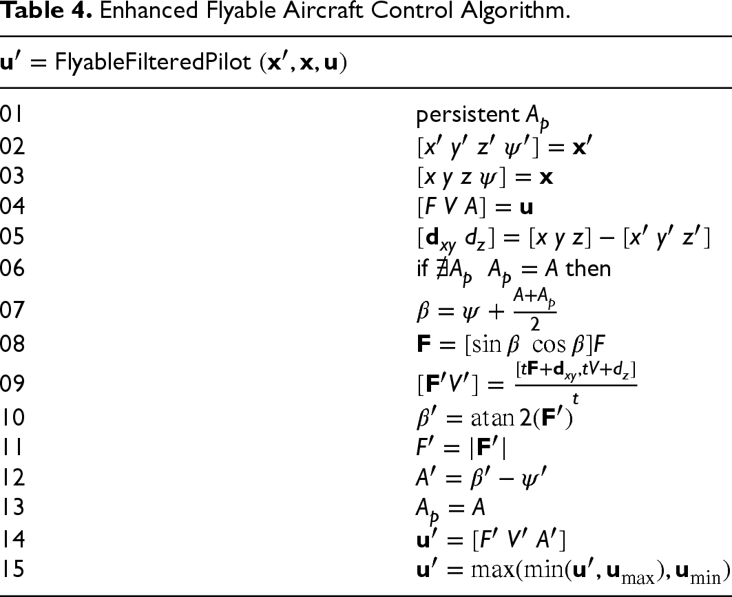
Table 4 shows an enhanced version of the model of pilot behavior presented in Table 3, in which the heading tracking is performed on the average between the last two references provided, in order to filter out those oscillations (07).

Table 4.
Enhanced Flyable Aircraft Control Algorithm.

$u^{'} =$ FlyableFilteredPilot $(x^{'}, x, u)$

01 persistent $A_{p}$

02 $[x^{'} y^{'} z^{'} ψ^{'}] = x^{'}$

03 $[x y z ψ] = x$

04 $[F V A] = u$

05 $[d_{x y} d_{z}] = [x y z] - [x^{'} y^{'} z^{'}]$

06 if $∄ A_{p} A_{p} = A$ then

07 $β = ψ + \frac{A + A_{p}}{2}$

08 $F = [\sin β \cos β] F$

09 $[F^{'} V^{'}] = \frac{[t F + d_{x y}, t V + d_{z}]}{t}$

10 $β^{'} = atan 2 (F^{'})$

11 $F^{'} = | F^{'} |$

12 $A^{'} = β^{'} - ψ^{'}$

13 $A_{p} = A$

14 $u^{'} = [F^{'} V^{'} A^{'}]$

15 $u^{'} = max (min (u^{'}, u_{max}), u_{min})$

$u^{'} =$ FlyableFilteredPilot $(x^{'}, x, u)$
01	persistent $A_{p}$
02	$[x^{'} y^{'} z^{'} ψ^{'}] = x^{'}$
03	$[x y z ψ] = x$
04	$[F V A] = u$
05	$[d_{x y} d_{z}] = [x y z] - [x^{'} y^{'} z^{'}]$
06	if $∄ A_{p} A_{p} = A$ then
07	$β = ψ + \frac{A + A_{p}}{2}$
08	$F = [\sin β \cos β] F$
09	$[F^{'} V^{'}] = \frac{[t F + d_{x y}, t V + d_{z}]}{t}$
10	$β^{'} = atan 2 (F^{'})$
11	$F^{'} = \| F^{'} \|$
12	$A^{'} = β^{'} - ψ^{'}$
13	$A_{p} = A$
14	$u^{'} = [F^{'} V^{'} A^{'}]$
15	$u^{'} = max (min (u^{'}, u_{max}), u_{min})$

Previous heading data is maintained by means of a persistent variable (01), the value of which is maintained between successive calls to the function. On the first call to the function, this value is initialized to current aircraft heading (06). Subsequently, this value is updated to indicate the previous course for successive function calls (13).

4. Performance Evaluation

As previously indicated, simulation was employed to validate and assess the performance of our proposed methodologies. In this section, we provide an initial overview of the simulation environment employed, followed by a comprehensive presentation and analysis of the obtained results.

4.1. Simulator Description

The simulator (Figure 12) has been developed in MATLAB/Simulink R2022a (The MathWorks Inc., 2025, 2025a), taking advantage of the available continuous and discrete-event simulation resources. It reflects the essential aspects of the approach and landing maneuver of an aircraft to a specific airport runway. The ATC block models the behavior of an air traffic controller who communicates with aircraft. From the information provided by the RADAR, it indicates them when to transit from one waypoint to the next in the descent maneuver, executing the algorithm presented in Table 1. The upper section of the Aircraft simulator is responsible for generating and consuming a discrete event that triggers the lower part, which contains the continuous systems modeling the real and the reference aircraft. The simulator supports the flow of multiple aircraft performing different approach manoeuvers. However, in this work, it is sufficient to analyze the behavior of the aircraft in isolation. At the bottom we can see two areas containing the continuous models of Dubins aircraft and Flyable aircraft. In both cases, Stateflow blocks define their respective behavior by means of state machines.

Figure 12.

Main section of the simulator.

Figure 13(a) shows the Dubins pilot state machine, whose purpose is reaching the current fly-by waypoint requested by the ATC. For this purpose, the machine executes two independent super-states in parallel. On the one hand, the COMMUNICATIONS state manages communications with the ATC, updating the target waypoint at the latter’s indication, also, this subsystem updates the information showed in the RADAR screen (Figure 2). Furthermore, the NAVIGATOR subsystem incorporates the state FLYING executing a function fly that implements the behavior defined in Table 2.

Figure 13.

Aircraft autopilots.

Figure 13(b) shows the flyable pilot state machine. In this case, the task of the autopilot system is limited to following the Dubins aircraft. To achieve it, the state FLYING executes a function follow that implements both behaviours defined in Table 3 and Table 4. Consequently, the communications subsystem does not interact with the ATC, limiting itself to update the position of the aircraft on the RADAR.

The Dubins aircraft dynamics block is detailed in Figure 14(a). Four continuous integrators (INTpsi, INTx, INTy, INTz) located in the left of the diagram convert the commanded velocities (sent by the autopilot) into variations in position orientation of the aircraft. The discrete retainer has no explicit function. It is used to synchronize all output signals provided by the system. Additionally, the aircraft dynamics block is detailed in Figure 14. The flyable behavior is implemented by means of second-order actuators, which smoothly evolve the actual speeds until they match the commanded speeds. These actuators have been configured to emulate the performance of a category C aircraft.

Figure 14.

Aircraft dynamics.

4.2. Approaching Procedure

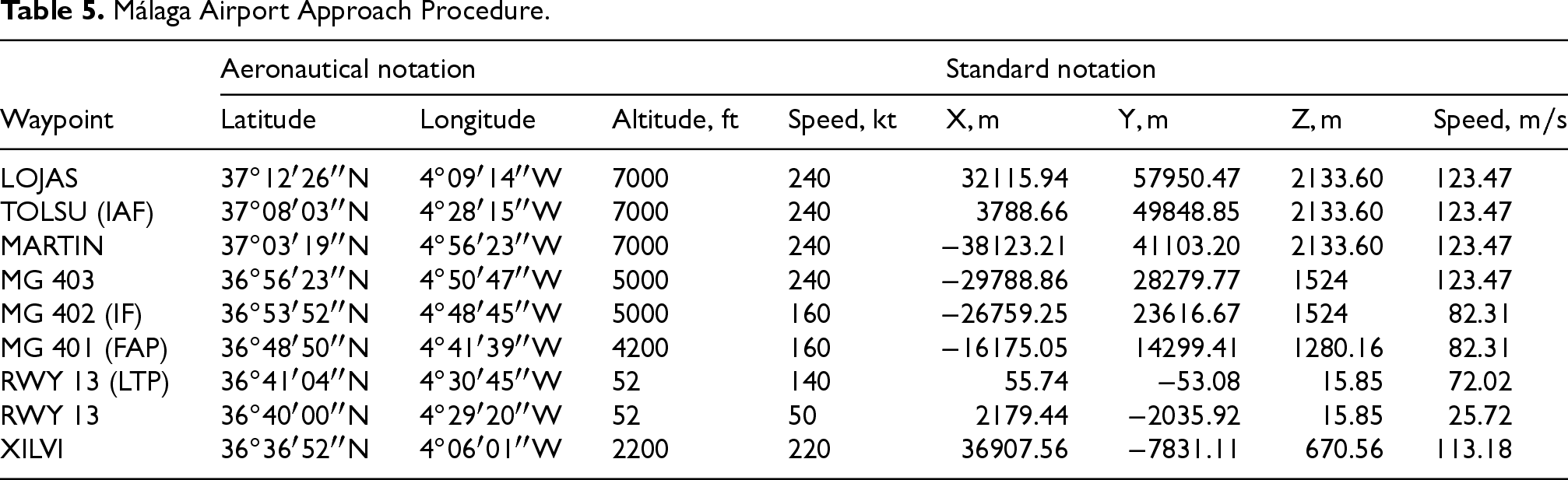
The described simulator can execute any approach maneuver, conveniently defined by a sequence of waypoints. In this work, we have considered the runway “RWY 13” of Malaga airport (Spain), shown in Figure 15 and summarized in Table 5.

Figure 15.

Málaga “RWY 13” approach procedure.

Table 5.

Málaga Airport Approach Procedure.

	Aeronautical notation				Standard notation
Waypoint	Latitude	Longitude	Altitude, $ft$	Speed, $kt$	$X, m$	$Y, m$	$Z, m$	Speed, $m / s$
LOJAS	$37^{\circ} 12^{'} 26^{″} N$	$4^{\circ} 09^{'} 14^{″} W$	7000	240	32115.94	57950.47	2133.60	123.47
TOLSU (IAF)	$37^{\circ} 08^{'} 03^{″} N$	$4^{\circ} 28^{'} 15^{″} W$	7000	240	3788.66	49848.85	2133.60	123.47
MARTIN	$37^{\circ} 03^{'} 19^{″} N$	$4^{\circ} 56^{'} 23^{″} W$	7000	240	$- 38123.21$	41103.20	2133.60	123.47
MG 403	$36^{\circ} 56^{'} 23^{″} N$	$4^{\circ} 50^{'} 47^{″} W$	5000	240	$- 29788.86$	28279.77	1524	123.47
MG 402 (IF)	$36^{\circ} 53^{'} 52^{″} N$	$4^{\circ} 48^{'} 45^{″} W$	5000	160	$- 26759.25$	23616.67	1524	82.31
MG 401 (FAP)	$36^{\circ} 48^{'} 50^{″} N$	$4^{\circ} 41^{'} 39^{″} W$	4200	160	$- 16175.05$	14299.41	1280.16	82.31
RWY 13 (LTP)	$36^{\circ} 41^{'} 04^{″} N$	$4^{\circ} 30^{'} 45^{″} W$	52	140	55.74	$- 53.08$	15.85	72.02
RWY 13	$36^{\circ} 40^{'} 00^{″} N$	$4^{\circ} 29^{'} 20^{″} W$	52	50	2179.44	$- 2035.92$	15.85	25.72
XILVI	$36^{\circ} 36^{'} 52^{″} N$	$4^{\circ} 06^{'} 01^{″} W$	2200	220	36907.56	$- 7831.11$	670.56	113.18

Figure 16.

Aircraft approaching maneuver.

Figure 17.

Straight-line course correction.

Figure 18.

Course correction at MARTIN Waypoint.

Waypoint XILVI is related to missed approach manoeuvers and is not relevant in this work. The blue line shows the sequence of waypoints. The green line represents the runway. According to the procedure (which also contemplates other possibilities), the aircraft (red point) enters the airspace through the LOJAS waypoint, heading for TOLSU. It then heads for MARTIN, where it turns to port and reduces height. At the final approach fix MG401, the last phase of the approach began, reaching the landing threshold point RWY13.

4.3. Simulation Results

After describing the simulation environment this section presents the obtained results. Firstly, Figure 16 depicts the accuracy of our proposed autopilot systems in tracking a reference aircraft executing the previously described runway approach maneuxer, The figure comprises four plots, with the first three presenting aircraft altitude, heading, and forward speed, respectively. Each plot contains series for both the Dubins reference aircraft trajectory and an application of a Kalman Filter to smoothen the trajectory-an established method documented in the literature (Kalman, 1960). Additionally, two series illustrate the bebavier of our original and enhanced tracking proposals. The last plot contains only 3 series showing the error made by these proposals in the tracking of the Dubins reference. In all cases, the horizontal axis is common and represents time of flight. As outlined in Table 5, initially the reference aircraft maintains an altitude of $7000 ft$ , a course $ψ = 254^{\circ}$ , and a speed of $240 kt$ . A small course correction occurs in TOLSU (at $240 s$ ). After passing MARTIN (at $553 s$ ), the reference aircraft turns to port while descending towards the waypoint MG403. The turn is completed at heading $ψ = 143^{\circ}$ (at $598 s$ ). On reaching $5000 ft$ (at $685 s$ ) the descent is completed, and the Dubins aircraft stabilises again. At this point, the aircraft reduces its speed. Later (at $760 s$ ), over waypointMG402, another small turn is made, and the aircraft is aligned with the runway. Next, it descends to $4200 ft$ reaching the final approach point (at $923 s$ ). Lastly, it reduces its speed again and proceed to land at time $1225 s$ .

Finally, the last plot of Figure 16 illustrates the tracking error exhibited by the flyable aircraft following the reference aircraft. It is observed that the Dubins, aircraft executes a non-flyable manoeuvre, entailing an abrupt transition from straight-line flight to a curved trajectory with a specified radius. In contrast, flyable aircraft must reach this radius of curvature progressively, requiring a few seconds to do so. The consequence is an error of $101 m$ for the basic tracking system, and $82 m$ for the enhanced tracking system. In this instance, the Kalman filter’s response is delayed, thereby failing to effectively compensate for the error and exacerbating it to $231 m$ . The turn maneuxer demands approximately $50 s$ for completion, and the tracking systems require nearly twice that time to rectify the resultant tracking error. Moreover, additional errors stemming from inertial effects during speed reduction are notable across the three phases in which they occur. Specifically, the last phase (at $1229 s$ ) is irrelevant, because it occurs at final braking, with the aircraft taxiing down the runway.

Figure 17 (above) shows a detail corresponding to a moment when the aircraft is flying in a straight line $(400 s)$ . We can observe how the Dubins reference aircraft does not fly exactly in a straight line, making small corrections to left and right alternately. This is because the autopilot is executed once per second, and the preset radius curve performed in that time does not leave the aircraft exactly aligned with the destination waypoint. In practice, the aircraft maintains a straight line with an error of less than $3^{\circ}$ . The original tracking system manages to filter out these oscillations by significantly reducing their frequency, at the cost of slightly increasing their amplitude. For its part, the inertia implemented in the improved tracking system perfectly dampens these oscillations by significantly reducing both frequency and amplitude; and the same is true for the variant incorporating a Kalman filter. Figure 17 (below) shows how the error becomes less than $10 m$ for the original autopilot system and less than $2 m$ for the improved autopilot and Kalman systems. We assume that aircraft immediately adapt their forward speed to that specified by the current waypoint and then hold it steady until they reach that waypoint. In the third plot of Figure 16 we can see this behaviour. The reference aircraft makes 3 instantaneous reductions, whereas the flyable aircraft require a few seconds to adapt their velocities. Additionally, we can observe the speed corrections (both accelerations and reductions) that flyable aircraft make when tracking the reference. In particular, after the turn at MARTIN, the flyable aircraft have fallen somewhat behind and a slight increase in their forward speed is noticeable (at $600 s$ ). After that, at each speed reduction (at $695 s$ , $929 s$ , and $1230 s$ ), flyable aircraft react more slowly than the reference aircraft, overtaking it. Consequently, when they reduce speed, they do so to a greater extent, to progressively correct the situation a posteriori.

The most significant errors occur in steep turns, such as the one performed at MARTIN (at $568 s$ ). A detail of this manoeuvre is presented in Figure 18. The upper plot shows the heading followed by the aircraft over time. The lower plot shows the relative error made by the 3 proposals with respect to the initial reference. It is clearly seen how the original tracker makes an error that it subsequently compensates for. On the other hand, the improved tracker acts faster, making a smaller error that requires less compensation. Finally, it can be seen that the Kalman filter acts more slowly and does not manage to compensate for the deviation until the end of the maneuver when the aircraft returns to a straight line.

5. Conclusions

This paper deals with the use of runway approach procedures based on Dubins trajectories, as well as their $4 D$ tracking by an aircraft. A method is proposed to define a fictitious aircraft that will describe the Dubins trajectory by generating a 4D reference, and two tracking mechanisms (basic and improved) of this reference, which can be used by real aircraft. The mechanisms have been evaluated under ideal conditions (in the absence of turbulence), verifying their correct operation and their high tracking accuracy. Compared to a Kalman filter, our improved mechanism achieves equal straight-line performance, but much better behavior during course change manoeuvers.

As future work, we propose, firstly, to modify our model to support progressive horizontal speed variation, which will most likely result in a reduction of error committed by this cause in the tracking of the reference. Furthermore, we propose to optimize the approach procedures by replacing the Dubins trajectories (non-flyable) with clothoid trajectories (flyable), which will also contribute to reducing the error committed in the turning manoeuvers.

Footnotes

Funding

This work is supported by R&D projects PID2021-123627OB-C52 and PLEC2023-010348, funded by MCIN/AEI/10.13039/501100011033 and “ERDF A way of making Europe”, and by the Universidad de Castilla—La Mancha under grant 2023-GRIN-34056.

Declaration of Conflicting Interests

The author(s) declared no potential conflicts of interest with respect to the research, authorship and/or publication of this article.

ORCID iDs

Wafae Azoulay

Rafael Casado

Abdelkrim Haqiq

Aurelio Bermúdez

Luis Orozco-Barbosa

Appendix

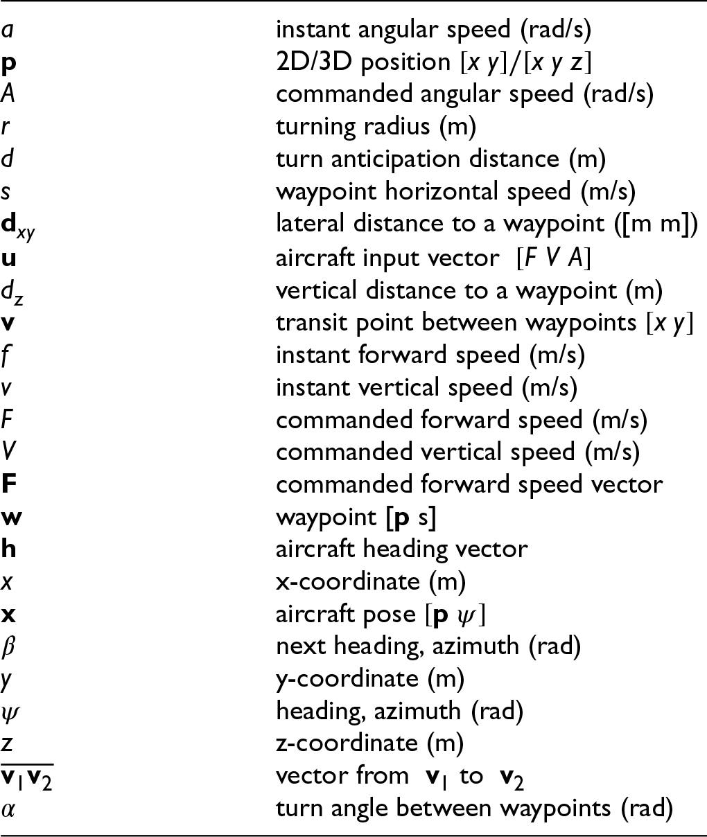
$a$	instant angular speed (rad/s)
$p$	2D/3D position $[x y] / [x y z]$
$A$	commanded angular speed (rad/s)
$r$	turning radius ( $m$ )
$d$	turn anticipation distance (m)
$s$	waypoint horizontal speed (m/s)
$d_{x y}$	lateral distance to a waypoint ([m m])
$u$	aircraft input vector $[F V A]$
$d_{z}$	vertical distance to a waypoint (m)
$v$	transit point between waypoints $[x y]$
$f$	instant forward speed ( $m$ / $s$ )
$v$	instant vertical speed ( $m$ / $s$ )
$F$	commanded forward speed (m/s)
$V$	commanded vertical speed ( $m$ / $s$ )
$F$	commanded forward speed vector
$w$	waypoint [ $p$ s]
$h$	aircraft heading vector
$x$	x-coordinate (m)
$x$	aircraft pose $[p ψ]$
$β$	next heading, azimuth (rad)
$y$	y-coordinate (m)
$ψ$	heading, azimuth (rad)
$z$	z-coordinate (m)
$\bar{v_{1} v_{2}}$	vector from $v_{1}$ to $v_{2}$
$α$	turn angle between waypoints (rad)

References

Bureau

A. T.

(2020). Effects of novel coronavirus (COVID-19) on civil aviation: Economic impact analysis. International civil aviation organization (ICAO), Montréal, Canada (p. 178).

Casado

López-Lago

Serna

Bermúdez

(2021). Enhanced missed approach procedure based on aircraft reinjection. IEEE Transactions on Aerospace and Electronic Systems (IEEE), 57, 4149–4170.

Chen

Tang

Wang

(2023). A study of collaborative trajectory planning method based on starling swarm bionic algorithm for multi-unmanned aerial vehicle. Applied Sciences (MDPI), 13, 6795.

De Jong

de Vos

Borst

van Paassen

Mulder

(2011). Time-based spacing for 4D approaches using speed-profiles. In AIAA guidance, navigation, and control conference, Montréal (pp. 6215). Canada.

Dubins

L. E.

(1957). On curves of minimal length with a constraint on average curvature, and with prescribed initial and terminal positions and tangents. American Journal of mathematics (JSTOR), 79, 497–516.

Enea

Porretta

(2012). A comparison of 4D-trajectory operations envisioned for Nextgen and SESAR, some preliminary findings. In 28th Congress of the international council of the aeronautical sciences (Vol. 5, pp. 4152–4165).

Guan

Sun

Liu

(2016). A study of 4D trajectory prediction based on machine deep learning. In 2016 12th World congress on intelligent control and automation (WCICA) IEEE (pp. 24–27).

Guan

Zhang

Chen

Michal

(2017). A large-scale multi-objective flights conflict avoidance approach supporting 4D trajectory operation. Science China Information Sciences (Springer), 60, 1–13.

Haghighi

Delahaye

Asadi

(2022). Performance-based emergency landing trajectory planning applying meta-heuristic and dubins paths. Applied Soft Computing(Elsevier), 117, 108453.

10.

International Civil Aviation Organization (ICAO). (2009). Required Navigation Performance Authorization Required (RNP AR) Procedure Design Manual. ICAO.

11.

International Civil Aviation Organization (ICAO). (2016). 4444–Procedures for Air Navigation Services–Air Traffic Management. Montreal, QC, Canada: The International Civil Aviation Organization (ICAO).

12.

Kalman

R. E.

(1960). A new approach to linear filtering and prediction problems. Transactions of the ASME – Journal of Basic Engineering, 82, 35–45.

13.

Klooster

Wichman

Bleeker

(2008). 4D trajectory and time-of-arrival control to enable continuous descent arrivals. In AIAA Guidance, navigation and control conference and exhibit (p. 7402).

14.

Lin

Saripalli

(2014). Path planning using 3D dubins curve for unmanned aerial vehicles. In 2014 international conference on unmanned aircraft systems (ICUAS) IEEE (pp. 296–304).

15.

López-Lago

Serna

Casado

Bermúdez

(2020). Present and future of air navigation: PBN operations and supporting technologies. International Journal of Aeronautical and Space Sciences (Springer), 21, 451–468.

16.

Núñez

H. E.

Camino

F. M.

Bouadi

(2017). Towards 4D trajectory tracking for transport aircrafts. IFAC-PapersOnLine (Elsevier), 50, 8196–8201.

17.

Pleter

Constantinescu

Stefanescu

(2009). Objective function for 4-D trajectory optimization in trajectory based operations. In AIAA guidance, navigation, and control conference (p. 6166).

18.

The MathWorks Inc. (2025). (n.d.-a) Retrieved May 28 from https://www.mathworks.com Matlab.

19.

The MathWorks Inc. (2025a). (n.d.-b) Retrieved May 28 from https://www.mathworks.com/products/simulink.html Simulink.