Machine learning in anesthesiology: Detecting adverse events in clinical practice

Abstract

The credibility of threshold-based alarms in anesthesia monitors is low and most of the warnings they produce are not informative. This study aims to show that Machine Learning techniques have a potential to generate meaningful alarms during general anesthesia without putting constraints on the type of procedure. Two distinct approaches were tested – Complication Detection and Anomaly Detection. The former is a generic supervised learning problem and for this a simple feed-forward Neural Network performed best. For the latter, we used an Encoder-Decoder Long Short-Term Memory architecture that does not require a large manually-labeled dataset. We show this approach to be more flexible and in the spirit of Explainable Artificial Intelligence, offering greater potential for future improvement.

Keywords

anesthesiology monitoring machine learning decision support system

Introduction

During clinical procedures, anesthesiologists rely on measurements displayed on ventilator and patient vital signs monitors. These have built-in alarm systems for critical incidents which produce warnings when a preset threshold is surpassed. Several studies have shown that a large number of false positives can occur. In moderate-risk operations, 64% of the alarms were labeled as clinically irrelevant, with only 5% requiring immediate action.¹ In high-risk cardiac surgery, 80% of alarms were considered useless.² There are a number of negative consequences that can arise from a high rate of false alarms. For example, anesthesiologists can become less sensitive to alarms if they occur unnecessarily. When they are occupied with another activity, they show decreased performance at interpreting the relevance of an alarm.³ Discomfort induced by a high false alarm rate, also known as “alarm fatigue”,⁴ can result in anesthesiologists changing the thresholds to more liberal values, or ignoring them entirely. Over 70% of anesthesiologists turn off the alarming systems due to an excess of false warnings.⁵

Methods from Artificial Intelligence (AI) have been tried as early as the 1990s to reduce the number of false alarms. Rule-based systems are built on expert knowledge and applied in a new context^6,7 and have yielded promising results in detecting a large number of critical patients states. However, they have failed to be broadly applied in practice because their optimization is cumbersome and such methods often failed to fully embrace the complexity of anesthesiology.⁸ Newer approaches apply Machine Learning (ML) algorithms, in which statistical dependencies in the data are identified through a training process to classify true complications. Rejab et al.⁹ used k-Prototypes Clustering to find groups of similar patients. For each group, they trained a ML classifier (Incremental Support Vector Machines) to monitor patients’ vital parameters and to generate appropriate alarms. This resulted in a reduction of 99.8% for false alarms and 97% for warnings. Hatib et al.¹⁰ used a ML classification algorithm called Logistic Regression to predict hypotension from early alterations in high-frequency arterial pressure waveforms. The algorithm was able to detect a hypotensive event 15 min in advance with 95% accuracy. This significantly reduced the average time and depth of hypotension in elective noncardiac surgeries, and this finding was reproduced in a follow-up study by Wijnberge et al.¹¹ In 2018, Kendale et al.¹² compared different ML classification algorithms in predicting the occurrence of peri-operative hypotension based on preoperative patient data. They found that Linear Discriminant Analysis, Gradient Boosting Machines, Neural Networks, and Random Forests are the best performing methods to predict the chance of hypotension (low blood pressure) during perioperative anesthesia.

There is an issue with transparency when applying ML techniques to healthcare. Most ML methods are intractable: it cannot be determined or explained how a classifier algorithm reached a specific result. There are also potential legal issues because the European General Data Protection Regulation (GDPR 2016/679 and ISO/IEC 27,001) makes it difficult to use black-box solutions in practice. The concept of Explainable-AI has been advanced that AI decision processes should be retraceable and interpretable.¹³ Choi et al.¹⁴ developed a promising algorithm with respect to transparency based on a Recurrent Neural Network. They used a special mechanism called Attention that determines what the most crucial “visits” and variables within a visit were, which are then displayed to the clinician to explain the reasoning behind a proposed medical diagnosis.

Although ML techniques seem very promising, no studies exist where ML has actually been used for health monitoring during routine anesthesia practice. We therefore tested multiple ML techniques to investigate whether they can be applied to a realistic clinical dataset, ranging from complex black-boxes to more simple semi-transparent solutions. In this paper, we focus only on a selection, which we believe to be the most relevant for the given problem. We aim to outline the general idea of applying AI to health monitoring rather than presenting a single fined-tuned solution. We studied and compared two distinct approaches, namely Complication Detection and Anomaly Detection, which vary in required input (labeled vs. unlabeled) and output (specific vs. general indication of an adverse event).

Methods

Data

Data for this project was provided by the Department of Anesthesiology of University Medical Center Groningen (UMCG). The anonymized dataset consisted of a subset (n = 715) of clinical procedures performed between 2014 and 2017. Due to the retrospective character of the project, the use of anonymous data, and because patients were not subject to intervention, our medical ethical committee waived the need for informed consent (UMCG Ethics’ Committee, METC 2020/624).

The measurements were sampled every 15 s (0.067 Hz) and contained vital parameters which were used as input variables for the ML models: HR (Heart Rate), EtCO₂ (End-Tidal Carbon Dioxide), FiO₂ (Fraction of inspired Oxygen), TVE (Tidal Volume Expired), Respiratory Rate, SpO₂ (Oxygen Saturation), P_max (Peak Inspiratory Pressure), PEEP (Positive End-Expiratory Pressure), Temperature, ABP_sys (Systolic Arterial Blood Pressure), ABP_dia (Diastolic Arterial Blood Pressure), MAP (Mean Arterial Pressure), C_dyn (Dynamic Lung Compliance) and body weight. Since most ML algorithms operate on windowed time-series data, the datasets were processed to such a format with a duration of 10 min. This value was chosen based on consultation with physician anesthesiologists. Hence, the dimensions of a single sliding window were 40 timesteps x 14 features.

Complication detection approach

In Complication Detection, a classifier algorithm was trained to detect a medical complication, in this case hypotension. Even though it has no rigorous definition, hypotension is thought to occur in 41%–93% of all procedures¹⁵ and posits danger for patient health if undetected. Cases where hypotension was detected by the anesthesiologist and officially registered as complication were selected. Data preprocessing consisted of: (1) perioperative phase selection based on the use of mechanical ventilation; (2) blood pressure measurement selection – when available, arterial blood pressure was chosen over the less precise noninvasive method with an arm cuff; (3) missing data imputation with polynomial interpolation; (4) standardization was achieved using median centering per patient and rescaling the so that the 25^th and 75^th quantiles fall within −1 to 1 range. The selected 83 procedures consisted of over 46 000 time steps (200 h) where 21% of the time steps were labeled as hypotensive.

It was not technically feasible to have an expert manually flag all hypotensive events so the detection of hypotension used Ballast’s⁶ rule-based system as the ground truth for our ML models. This system uses mathematical expressions based on expert knowledge (Figure 1) to indicate the time of occurrence of a complication. For each time step, the algorithm computes the complication indicators using factors such as moving averages of past observations measured in different periods, the time for which a threshold was surpassed by some vital parameter, and relationships between the parameters. The hypotension alarm used in the current study was generated by two sets of equations. The first checks if ABP_sys < 70 mm Hg. The second set is responsible for monitoring the trend of consecutive measurements, which is done by first establishing a threshold for an acceptable relative rate of change in ABP_sys. This threshold has a gradually decreasing tolerance to changes depending on the proximity of ABP_sys to the 70 mm Hg boundary. For every incoming measurement of ABP_sys, moving averages are calculated with time constants of 20, 200 and 2000 seconds. This allows determination whether the blood pressure is falling at a fast, medium or slow speed. If any of these trend indicators surpasses a certain change threshold, or if the absolute ABP_sys from the first equation is too low, then the hypotension alarm is triggered.

Figure 1.

Rule-based system label generation.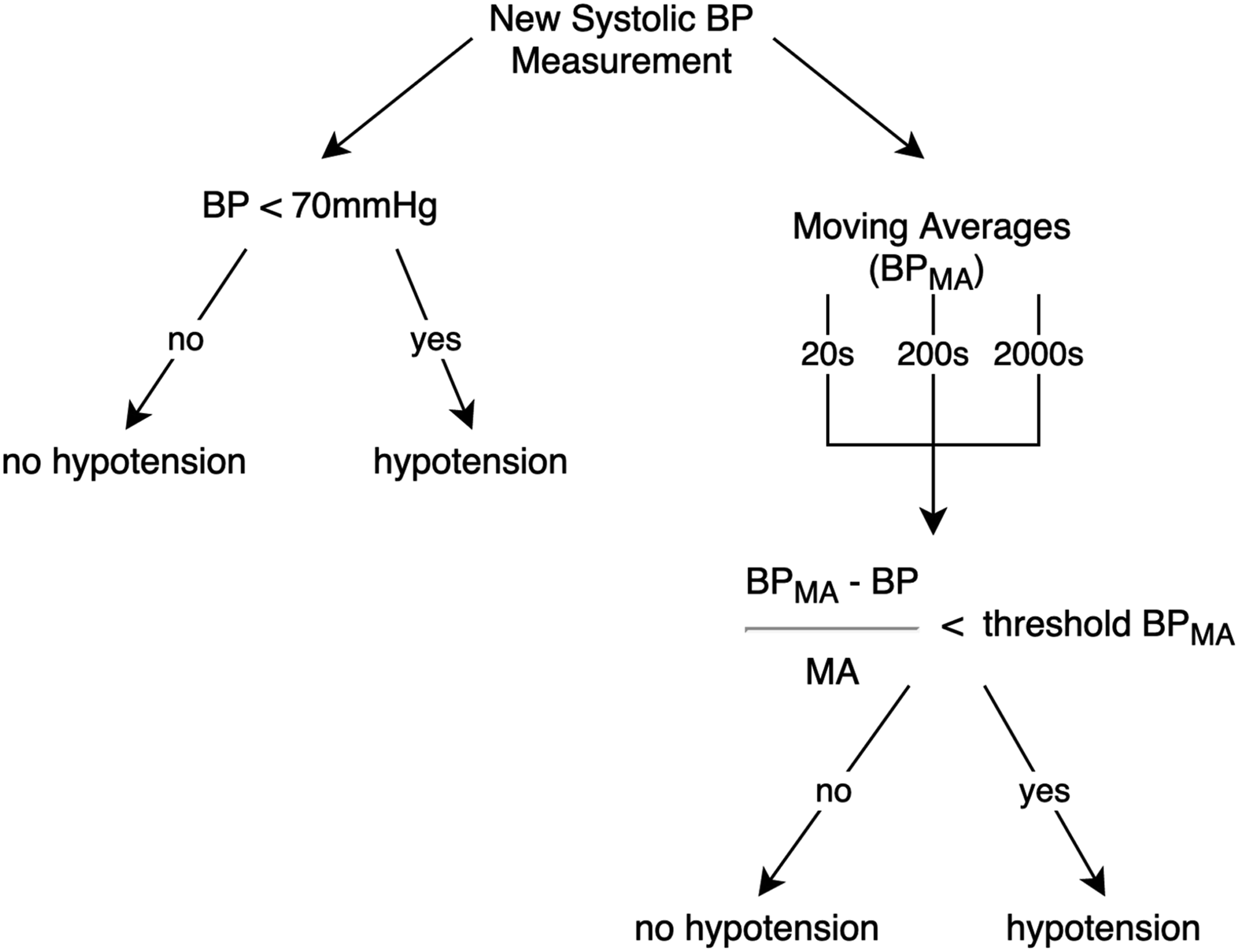

In our Complication Detection approach, we tested two ML algorithms: Random Forest and Fully Connected Neural Network – these handle windowed time series data in a different way.

Random Forest is an ensemble of Decision Trees, one of the simplest ML techniques. It is constructed from true/false nodes which ask questions about the data until the samples from the training set have been split in a way that the last nodes contain samples of only one class. It is common practice to train multiple Decision Trees (a Forest) on random subsets of the full dataset and take their averaged prediction. This additional randomness helps the Forest to generalize better over the data, whereas a Decision Tree is often biased by noise in the training dataset. A Tree is a fully-transparent algorithm – the exact steps it took to make a decision can be traced-back, but the Forest is a semi-transparent algorithm – one can check which features on average contribute most to making the splits. Random Forests cannot process time-dependent relations, thus additional time-based features were extracted from the dataset. This was done with a Python package called TSFRESH¹⁶ which extracts features (e.g. mean, entropy, number of peaks, etc.) from the windowed time-series that carry relevant information for predicting the dependent variable. The reconceptualization of the data resulted in 3604 new features instead of the 14 standard sequential variables.

Neural Networks (ANNs or NNs) are another family of ML algorithms, which are inspired by the physiology of the human brain. They typically contain thousands of artificial neurons organized in layers similarly to the cortical architecture. These algorithms work directly on the time-series data, so extraction of time-based features is not necessary. NNs are capable of capturing the non-linear processes that occur in the real world and this has contributed to their popularity in the last two decades. The learning process of a NN is based on iteration over training sets and adjusting the network weights and biases, so that a cost function is minimized. This is usually the difference between its outputs and the target variable. A Fully-Connected Feed-Forward Neural Network is a standard neural architecture with all its units in one layer connected to all units in the contiguous layers. The data flows from an input layer, through one or more hidden layers to an output layer. For the Complication Detection system, this is a single neuron that generates the probability that the vital parameters input to the network represent a hypotensive event.

Both algorithms were implemented using Python libraries (Scikit-learn and Keras with TensorFlow backend) and run on a Nvidia k40 GPU from the Peregrine HPC cluster. The models were trained and optimized on 85% of the data using 5-Fold Cross-Validation and the remaining 15% of the data was used for final tests – every operation was randomly assigned to one of the three subsets. The Random Forest was left at its default settings except for the number of trees/estimators which was set to 75. The Fully-Connected Feed-Forward Neural Network was trained using the Adam optimizer and log-loss cost function. The network (Figure 2) consisted of an input layer that flattened the sliding window to 560 values with a dropout rate of 0.2 applied to it. The hidden layer contained 700 units (dropout = 0.5, activation = ReLU) and the output was a single neuron with sigmoidal activation that generated the probability of hypotension.

Figure 2.

Fully-Connected Neural Network used in the Complication Detection approach.

Anomaly detection approach

Anomaly Detection was implemented by training a ML algorithm on a dataset with only non-complications cases. The resulting model should be able to fit the standard non-anomalous behavior of the vital parameters. Following this assumption, any measured value that does not match the predictions or expectations of the model is considered an anomaly. The dataset for this approach contained cases where the anesthesiologist present during the operation procedure flagged it in the record system as “no complications”, which means that no adverse event had occurred. Labeling every time step was necessary for this approach due to the model’s generative nature. After preprocessing, performed as in Complication Detection, the dataset consisted of 632 operations with roughly 500 000 timesteps (2000 h) in total. The input variables were the same 14 vital parameters as previously.

The Anomaly Detection approach was based on a study on multi-sensor data.¹⁷ A NN was trained to forecast a sequence of 16 future time steps (4 min) for each of the 13 vital parameters (we did not forecast body weight). The forecasting was approached with Sequence-to-Sequence modeling¹⁸ and more specifically an Encoder-Decoder Long Short-Term Memory Network (E-D LSTM). This architecture uses Long Short-Term Memory (LSTM) layers¹⁹ rather than the standard artificial neurons, as LSTMs have the ability to model time-dependent changes, a crucial property for forecasting sequences (Figure 3). In the Encoder part of our architecture, an LSTM layer generated the historical context of the whole sequence. The Decoder part used this context and the most recent input to recursively generate 16 future time steps with its LSTM layer. The forecasts from the E-D LSTM model were then accumulated at each time step and compared to the actual data. If the difference between the forecasts and the patient data exceeded a threshold (set in consultation with an anesthesiologist), an anomalous state was detected (see Appendix 1). Additionally, such an approach to Anomaly Detection based on forecasting error allows retrieving the source of abnormal changes in the current input by identifying which of the 13 vital parameters have the largest error.

Figure 3.

Encoder-Decoder LSTM architecture unfolded in time. Each LSTM instance contains bidirectional 64 units in the Encoder section and 128 units in the Decoder. Hollow arrows represent the LSTM state being passed in time and the solid arrows show the data flow beteween the inputs and outputs. Fully-Connected layers (FC) generate predictions of 13 vital parameters at each forcasted time step. Note: LSTM: Long Short-Term Memory.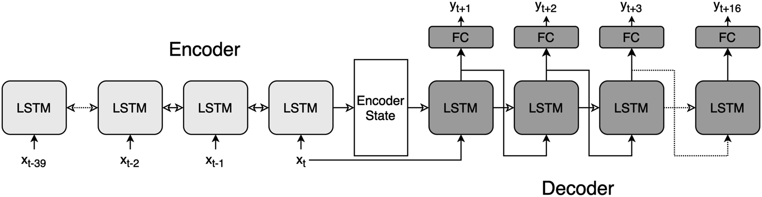

The Log-Cosh was used as loss function for the E-D LSTM and the Adam function as optimizer. The Encoder consisted of 64 Bidirectional LSTM units (dropout = 0.2; recurrent dropout = 0.2) and the Decoder was built out of 128 LSTM units (dropout = 0.2, recurrent dropout = 0.2) on top of which a fully-connected layer with 13 units with linear activation generated the forecasted values.

Metrics

The choice of metric determines which aspects of an alarming system are the most influential. For medical diagnosis, the priority is to consider the fraction of all hazardous events that are actually detected by the system, which is given by recall

R e c a l l = \frac{t r u e p o s i t i v e s}{t r u e p o s t i v e s + f a l s e n e g a t i v e s}

It is also necessary to register the fraction of all generated alarms that are true hazardous events, known as precision

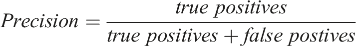
P r e c i s i o n = \frac{t r u e p o s i t i v e s}{t r u e p o s i t i v e s + f a l s e p o s t i v e s}

Together, recall and precision describe the completeness and exactness of an alarming system which is expressed as the F₁ score – a harmonic mean between the two

F_{1} = 2 \times \frac{p r e c i s i o n \times r e c a l l}{p r e c i s i o n + r e c a l l}

F₁ score is not directly interpretable but allows to easily compare models with regards to precision and recall without being biased by a high score of one of these two metrics. Moreover, since precision and recall formulas do not include true negatives – these are of little interest in medical diagnosis systems – they are more robust to class imbalance.²⁰ This is an important property because hypotensive events are underrepresented in our data compared to the more common non-hypotensive condition. Area Under ROC Curve was also computed for completeness; however, it should be considered with caution since is likely boosted by high recall score and class imbalance.

Results

For Complication Detection, a non-ML baseline was implemented to assess if the ML techniques based their decisions on the complex data patterns instead of simply predicting the most frequent class from the training set. A Positive Guess baseline was used which naively predicted for each time step the outcome “hypotension”. Each ML model was trained 5 times and evaluated on the test set to provide averaged final scores (Table 1).

Table 1.

Final scores for complication detection techniques.

Algorithm	Engineered features	Precision	Recall	F₁	AUC
Positive guess	N/A	0.21	1	0.35	0.50
Decision tree	Yes	0.28	0.57	0.38	0.64
Random forest	Yes	0.37	0.73	0.49	0.73
Fully-connected network	N/A	0.51	0.63	0.56	0.82

Note: AUC: Area Under ROC Curve.

All of the described techniques showed increased performance compared to the baseline (F₁ = 0.35) with the Decision Tree (F₁ = 0.38) and Random Forest (F₁ = 0.49) obtaining lower scores than the NN (F₁ = 0.56). Additionally, the precision-recall curve in Figure 4 depicts how recall and precision would change if the class assignment threshold (set by default to 0.5) was altered. It can be observed that for the NN to obtain a recall score of 1, precision would have to decrease to around 0.21, which is equal to the Positive Guess baseline score. Inspecting the most relevant features in the Random Forest indicated that its classification was mostly based on engineered features of the blood pressure measurements and more specifically the mean change inside the 10-min window.

Figure 4.

Precision-Recall curve of the Fully-Connected Neural Network.

For Anomaly Detection, a naive baseline, called Future Duplication, was used. At each time step t the most recent observation t-1 was duplicated to depict future predicted values at t + 1…t + 16. Mean Absolute Error (MAE) between the actual values of the vital parameters of 16 future time steps and their predicted values generated by the E-D LSTM were equal to 0.44 and 0.37 for the Future Duplication baseline, indicating that the forecasts of the ML algorithm showed decreased performance compared to the naively-generated ones (Table 2). Additionally, the E-D LSTM technique was tested on 10, previously unseen, procedures where an anesthesiologist tagged 1% of the time points as anomalous. In this test, the ML algorithm performed similarly (F₁ = 0.32) to the baseline (F₁ = 0.34).

Table 2.

Anomaly detection results.

		Future duplication	E-D LSTM
Forecast quality	MAE	0.37	0.44
Detection quality	Precision	0.22	0.2
	Recall	0.81	0.83
	F1	0.34	0.32

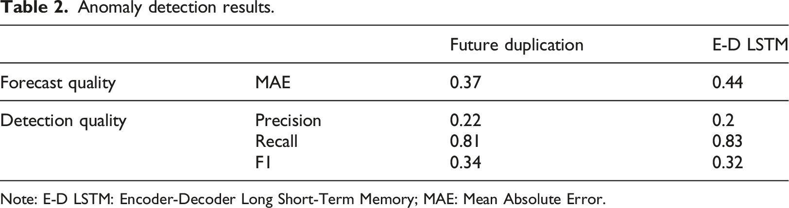
Note: E-D LSTM: Encoder-Decoder Long Short-Term Memory; MAE: Mean Absolute Error.

Discussion

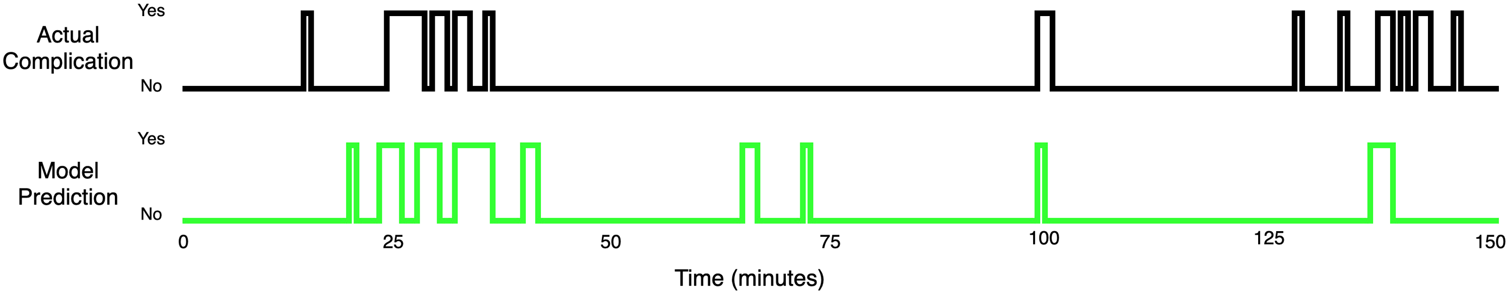
Although scores achieved in Complication Detection by the Random Forest and NN are not impressive, they show that these algorithms are capable of learning patterns that occur in the vital parameters. Visual inspection of the probabilistic outputs of the NN showed that detecting hypotension flagged by the rule-based system is generally an easy task for this ML technique. Anesthesia cases which contained fewer non-physiological artifacts were modeled almost perfectly by the NN and the resulting alarms were of high medical relevance in such cases (Appendices 2 and 3). More precisely, the cases where arterial blood pressures were measured invasively (with an intra-arterial canula) on a continuous base did not cause difficulties for the networks; fewer data points were missing compared to noninvasive interval measurements, and artifacts with a non-physiological background were not overwhelmingly present. One can imagine that if systems based on NNs were to be used during actual clinical procedures, the staff would have to ensure that the recorded data are reasonably uncorrupted. We believe that a dataset with a reasonable number of artifacts and reasonable time resolution (≤0.067 Hz) would allow future studies to obtain significant improvement in precision and recall scores, as our results were likely understated by the data imperfections. In case of the Random Forest, which clearly outperformed a single Decision Tree, another possible improvement would be replacing the Forest with an often more effective technique of optimizing multiple Decision Trees, namely Gradient Boosting Machine, and extracting the features manually in consultation with domain experts.

The Anomaly Detection method based on the averaged forecasting error seems to be a promising approach, although it managed to detect only the more obvious anomalies. This low sensitivity was caused by poor forecasting capabilities of the E-D LSTM – at least in their current setup, as it did not surpass the naive baseline. It must be clear that we do not expect a forecasting algorithm to achieve a MAE score close to 0, as that would indicate that the anomalies were also modeled and would be a sign of over-fitting in the Anomaly Detection. Nevertheless, a basic inspection of training and validation curves’ convergence showed that overfitting was not an issue in our experiments, hence the next step would be to expose the E-D LSTM to more data and increase the complexity of this model, for example by adding an Attention mechanism.²¹ Such improvements should theoretically help the neural architecture to capture better the patterns occurring in patient’s vital state. On the other hand, without high-fidelity recordings it is likely impossible to surpass a certain level of performance because some physiological phenomena are not observable in a lower time-resolution.

As for a comparison between the Complication and Anomaly Detection systems, even though Complication Detection seems a better performing approach at this point, it is unlikely that a complete alarming system could be based solely on it. To improve Complication Detection would require obtaining a training dataset with a sufficient number of labeled complications, but that would be a major obstacle. This obstacle becomes even more difficult when trying to detect complications less frequent than hypotension. A more realistic scenario would be to combine this ML learning approach with a rule-based system to obtain a product that offers the adaptiveness and sensitivity of the ML algorithms on the most often encountered complications, expanded by expert-defined complications that are well-known but rare.

Although a Decision Tree covered in the Complication Detection section is commonly referred to as a transparent method, it is not trivial to conceptualize its decision path into information that could be effortlessly and quickly interpreted in an operation room setting. Similarly, the feature weights from a Random Forest are more useful for describing the properties of the training dataset rather than the input’s during inference. The Anomaly Detection approach proved to be the more promising approach in this regard, as the ease of retrieving prediction errors per vital parameter (see Appendix 4. for an example) opens new possibilities for further development of such systems that are more in line with the concept of Explainable AI.¹³ Moreover, the fact that Anomaly Detection is based on methods that do not require a labeled training dataset should make it more generalizable across different patients and types of procedures. Anomaly Detection could also serve as a base for an alarming system by being responsible for the initial recognition of an abnormality in the incoming data stream. Such abnormality would then be processed by a rule-based system or any other classifier, such as our Complication Detection system, which could interpret the abnormality based either on the raw values of the vital parameters or/and the prediction errors. However, these speculations about the future applications are only valid if the quality of the forecasts improves.

Final conclusions

Alarm systems that achieve a perfect recall score while maintaining a small percentage of false alarms (high precision) seems implausible. The tradeoff between precision and recall seems acutely relevant in health monitoring and the unpredictable nature of the medical events accentuates its importance. To introduce impactful improvements for alarming systems, it is crucial to determine the implications of a small reduction in recall with a large increase in precision. Since anesthesiologists already tend to disregard alerts, it can be expected that the proposed changes will not impact the patient’s safety negatively and should increase the reliability of the whole system from the perspective of the medical staff.

We emphasize the need to reassess how alarming systems are viewed from a human-computer interaction perspective. We propose a shift from alert-generating devices to support systems that act as an additional staff member, but with a different type of intelligence that complements human cognition. If such conceptual change is possible then the methods offered by ML may provide the best solutions for generating reliable, generalized, and meaningful alarms.

Footnotes

Authors contributions

Study conception and design: TTM, KvA, AB, FC, MMRFS

Data preparation: TTM, KvA

Computational modelling: TTM, AB

Interpretation of data: TTM, KvA, AB, FC

Manuscript preparation: TTM, KvA, AB, FC, MMRFS

Declaration of conflicting interests

The author(s) declared the following potential conflicts of interest with respect to the research, authorship, and/or publication of this article: Michel MRF Struys: His research group/department received (over the last 3 years) research grants and consultancy fees from Masimo (Irvine, CA, USA), Becton Dickinson (Eysins, Switzerland), Fresenius (Bad Homburg, Germany), Dräger (Lübeck, Germany), Paion (Aachen, Germany), Medcaptain Europe (Andelst, The Netherlands). He receives royalties on intellectual property from Demed Medical (Temse, Belgium) and the Ghent University (Gent, Belgium). He is an editorial board member and Director for the British Journal of Anaesthesia and associate editor for Anesthesiology.

Funding

The author(s) received no financial support for the research, authorship, and/or publication of this article.

ORCID iDs

Tomasz T Maciag

Fokie Cnossen

Appendices (Digital Content)

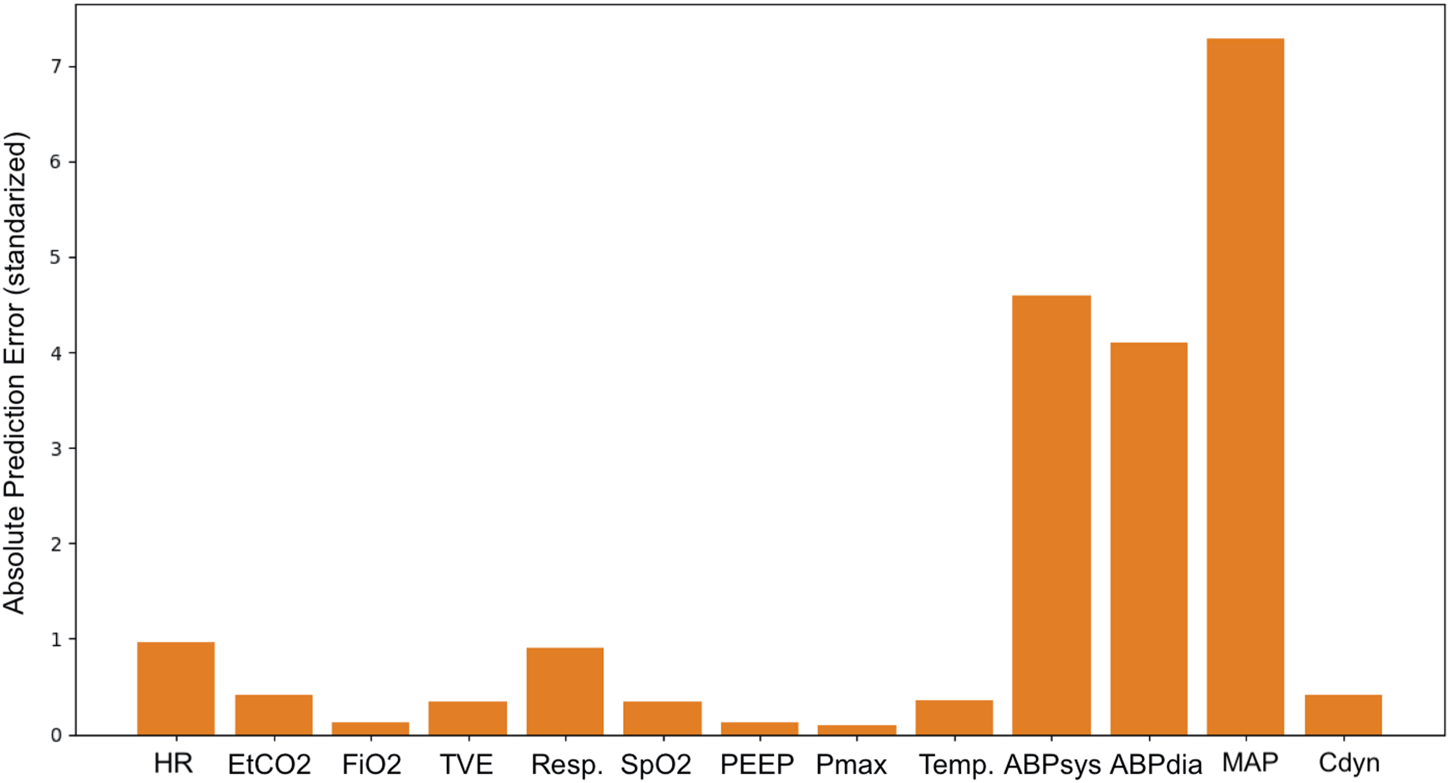
Appendix 1

The network was set to forecast l = 16 (4 min) future timesteps for each of the 13 vital parameters. These future predictions were accumulated, so that every timestep t was forecasted 16 times at t-16, t-15, …, t-1. Then, a prediction error was computed where e_ij^t is the absolute difference between x_i^t the actual value of the variable i measured at time t and its predicted value at time t-j. This means that for a given time step t there is an error vector e^t = [e_1,₁^t, …, ei₁_,l^t, …, e_d_,1^t, …, e_d,_l^t], where l is the number of future predictions, d is the number of dimensions (vital parameters). The next step was to average the error vectors across the l and d dimensions, so that for every timestep there would be only a single ē^t grand mean error value. Then, in order to provide a context for every ē^t, a median value was calculated from the last 8 steps median(ē^t-⁸ … ē^t-1) and summed with a constant threshold τ. Finding the optimal threshold was done by maximizing the F₁ score on the 10 expert-tagged operations from the validation set. Using a running median was motivated by the fact that some operations had periods which a NN could not model with a sufficient accuracy and had a generally higher prediction error ē^t. Also using a simple grand mean ē^t, rather than tracking each variable separately, provided more consistent results. To sum up, anomaly detection at time t was done by averaging all prediction errors e_d,l^t into ē^t and checking whether the following condition was violated ē < median(ē^t-⁸ … ē^t-1)+τ. To retrieve the prediction error per vital parameter, which we claim is an additional insight into the model’s decision, we simply display the 13 error vectors e^t averaged across the time dimension l (Appendix 4). Appendix 2.

Detections on good quality data.

Appendix 3.

Detections on poor quality data.

Appendix 4.

Encoder-Decoder Long Short-Term Memory’s absolute prediction errors on a hypotensive event. The scale of the error is an absolute value of the vital parameter standardized with the method described in the Data subsection.

References

de Man

Greuters

Boer

, et al. Intra-operative monitoring--many alarms with minor impact. Anaesthesia 2013; 68: 804–810.

Schmid

Goepfert

Kuhnt

, et al. The wolf is crying in the operating room: patient monitor and anesthesia workstation alarming patterns during cardiac surgery. Anesth Analg 2011; 112: 78–83.

Bliss

Dunn

. Behavioural implications of alarm mistrust as a function of task workload. Ergonomics 2000; 43: 1283–1300.

Röhrig

Timmer

Binder

. German Medical Data Sciences: Visions and Bridges Proceedings of the 62nd Annual Meeting of the German Association of Medical Informatics, Biometry and Epidemiology (gmds E.V.) 2017 in Oldenburg (Oldenburg) – GMDS 2017. Amsterdam, Netherlands: IOS Press, 2017.

Block

Nuutinen

Ballast

. Optimization of alarms: a study on alarm limits, alarm sounds, and false alarms, intended to reduce annoyance. J Clin Monit Comput 1999; 15: 75–83.

Ballast

. Warning Systems in Anesthesia. Doctoral Thesis. University of Groningen, 1992.

Sukuvaara

Koski

EMJ

Mäkivirta

, et al. A knowledge-based alarm system for monitoring cardiac operated patients — technical construction and evaluation. Int J Clin Monit Comput 1993; 10: 117–126.

Alexander

Joshi

. Anesthesiology, automation, and artificial intelligence. Bayl Univ Med Cent Proc 2017; 31: 1–3.

Rejab

Nouira

Trabelsi

. Health monitoring systems using machine learning techniques. In: Intelligent Systems for Science and Information. Cham: Springer, 2014, pp. 423–440.

10.

Hatib

Jian

Buddi

, et al. Machine-learning algorithm to predict hypotension based on high-fidelity arterial pressure waveform analysis. Anesthesiology 2018; 129: 1.

11.

Wijnberge

Geerts

Hol

, et al. Effect of a machine learning–derived early warning system for intraoperative hypotension vs standard care on depth and duration of intraoperative hypotension during elective noncardiac surgery: the hype randomized clinical trial. JAMA 2020; 323: 1052. DOI: 10.1001/jama.2020.0592.

12.

Kendale

Kulkarni

Rosenberg

, et al. Supervised machine learning predictive analytics for prediction of postinduction hypotension. Anesthesiology 2018; 129: 675–688.

13.

Holzinger

Biemann

Pattichis

, et al.

What do we need to build explainable AI systems for the medical domain?

ArXiv171209923 Cs Stat 2017, http://arxiv.org/abs/1712.09923 (accessed 19 September 2018).

14.

Choi

Bahadori

Kulas

, et al. RETAIN: An Interpretable Predictive Model for Healthcare using Reverse Time Attention Mechanism. ArXiv160805745 Cs, 2016, http://arxiv.org/abs/1608.05745 (accessed 19 September 2018).

15.

Bijker

Klei

WAvan

Kappen

, et al. Incidence of intraoperative hypotension as a function of the chosen definitionliterature definitions applied to a retrospective cohort using automated data collection. Anesthesiol J Am Soc Anesthesiol 2007; 107: 213–220.

16.

Christ

Braun

Neuffer

, et al. Time series feature extraction on basis of scalable hypothesis tests (tsfresh–A Python package). Neurocomputing 2018; 307: 72–77.

17.

Malhotra

Ramakrishnan

Anand

, et al. LSTM-based Encoder-Decoder for Multi-sensor Anomaly Detection. ArXiv160700148 Cs Stat, 2016, http://arxiv.org/abs/1607.00148 (accessed 7 December 2018).

18.

Sutskever

Vinyals

. Sequence to sequence learning with neural networks. In: Advances in Neural Information Processing Systems. Red Hook: NY Curran, 2014, pp. 3104–3112.

19.

Hochreiter

Schmidhuber

. Long short-term memory. Neural Comput 1997; 9: 1735–1780.

20.

Davis

Goadrich

. The relationship between Precision-Recall and ROC curves. In: Proceedings of the 23rd international conference on Machine learning - ICML ’06, Pittsburgh, Pennsylvania, 25 June 2006. ACM Press, pp. 233–240.

21.

Bahdanau

Cho

Bengio

. Neural Machine Translation by Jointly Learning to Align and Translate. ArXiv14090473 Cs Stat, 2014, http://arxiv.org/abs/1409.0473 (accessed 12 December 2018).