Lax pair and Darboux transformation for the generalized Fornberg–Whitham equation: Lump,breather,periodic,and rogue wave solutions

Abstract

In this article, we investigate a generalized Fornberg–Whitham (gFW) equation. Based on the Lax pair and Darboux transformation, one-soliton solution, breather solutions, lump solution, lump–1-strip, lump–periodic, manifold periodic, and rogue wave solutions for the gFW equation are obtained by choosing appropriate transformations and symbolic computation. In addition, we evaluate Ma breather, Kuznetsov–Ma breather and their corresponding rogue waves, generalized breather, and Akhmediev breathers. The obtained solutions reveal rich nonlinear wave phenomena such as localized structures, recurrence patterns, and energy concentration effects. These findings have direct applications in fluid dynamics, optical fiber communications, and plasma physics, where such nonlinear behaviors are prevalent. Moreover, the explicit construction of rogue waves and breather interactions provides insight into the prediction and control of extreme wave events in oceanography and nonlinear optics. The results further demonstrate the utility of analytical methods in exploring complex wave structures in integrable and near-integrable systems.

Keywords

nonlinear physics fornerg witham equation lax pair darboux transformation

1. Introduction

Nonlinear differential equations (NDEs) play a central role in the theory of solitons and arise in a wide range of disciplines within applied mathematics and engineering.^1–8 A fundamental aspect of this theory is the construction of analytical solitary wave solutions, which are essential for understanding the underlying dynamics of nonlinear systems. The continuous exploration of natural phenomena has further emphasized the importance of obtaining exact solutions of NDEs, particularly in the field of mathematical physics.^9–12 In this context, soliton theory has emerged as a powerful and active area of research with significant applications in materials science, plasma physics, optical fiber communications, and other branches of physical sciences.^13–17 Therefore, a variety of analytical techniques have been developed to construct exact solutions of proposed NDEs, including Bäcklund transformations,¹⁸ Painlevé analysis and Lie symmetries,¹⁹ spontaneous symmetry methods,²⁰ computational architectonics,²¹ and conservation laws.²² Moreover, several well-established approaches such as the extended tanh-function method,²³ Hirota bilinear scheme (HBS),²⁴ polynomial function method,²⁵ mapping techniques,²⁶ Lie symmetry analysis,27 and the CESTAC method²⁸ have proven effective in generating exact solutions. In addition, methods like symmetry bifurcation,²⁹ Kudryashov architectonics,³⁰ auxiliary equation methods,³¹ the (G′/G)-expansion method,³² semi-inverse techniques,³³ the $\exp (- φ^{'} / φ η)$ -expansion method,³⁴ as well as the homotopy perturbation method, direct algebraic methods, simplest equation techniques, and Lie symmetry-based approaches have also been widely employed to derive exact solutions of nonlinear differential equations. A recent works in the field of NDEs and various solutions, have been developed,^35,36 and the nonlinear problems in the field of structural analysis are potential field of applications.^37,38

The theory of integrable systems relies significantly on the Lax equation, which is essential to explaining how nonlinear partial differential equations (PDEs) evolve. This paradigm, which was first presented by Peter D. Lax, represents a nonlinear equation as the compatibility condition of two linear operators, referred to as a Lax pair (LP). In addition to displaying the integrable structure of the underlying PDE, this precise representation makes it easier to produce precise solutions. Lax pairings enable the use of strong algebraic methods like the Darboux transformation (DT) and the inverse scattering transform. Specifically, the DT is a straightforward technique that uses a series of transformations on the corresponding LP to produce new solutions from existing ones.^39–45 This method has demonstrated its importance in the larger study of nonlinear wave phenomena by being particularly successful in creating soliton, breather, and rogue wave solutions.

In this paper, our major intention is to get Lax pair, Darboux transformation, single-soliton solution, breather solutions, lump, lump 1-strip, lump-periodic, manifold periodic solution, rogue wave solutions of gFW-equation via choosing appropriate transformations and symbolic computation. In addition, we evaluate Ma breather, Kuznetsov–Ma breather and their corresponding rogue waves, generalized breather, and Akhmediev breathers. Therefore, gFW-equation is represented as,^46–49

u_{t} - u_{txx} + k u_{x} + m u u_{x} = \frac{9}{2} u_{x} u_{x x} + \frac{3}{2} u u_{xxx},

(1)

where u = u(x, t), while m > 0 and k are constants.

When k = −1 and m = 3/2 then Eq. (1) becomes the following Fornberg–Whitham equation,

u_{t} - u_{txx} - u_{x} + \frac{3}{2} u u_{x} = \frac{9}{2} u_{x} u_{x x} + \frac{3}{2} u u_{xxx} .

(2)

The novelty is we construct, for the first time, a systematic framework combining the Lax pair structure with the Darboux transformation for the gFW-equation, which has not been fully explored in the existing literature. We derive a wide spectrum of exact solutions within a unified analytical setting, including lump solutions, lump–1-strip, lump–periodic, manifold periodic waves, and multiple types of breather and rogue wave structures. The coexistence and interaction of these solutions in the gFW-system represent a novel contribution. We provide explicit constructions of higher-order and hybrid wave structures (such as lump–periodic and lump–stripe interactions), which reveal new dynamical behaviors not previously reported for this model. The study establishes connections between different classes of nonlinear waves (e.g., Ma breather, Akhmediev breather, and rogue waves) within the same mathematical framework, offering new insight into energy localization and transition mechanisms. Compared to existing studies that focus on isolated solution types, our work presents a comprehensive analysis of multiple nonlinear structures and their interactions, enhancing the understanding of complex wave dynamics in integrable and near-integrable systems.

The remaining structure of this manuscript is arranged as: In sec. 2, we compute the LP for governing model. In sec. 3, we will use Darboux theorem and DT on Eq. (2). In sec. 4, we will apply DT on the stated model to compute one-soliton solution. The sec. 5 provides a brief evaluations of lump wave results along with some 3D and contour illustrations. In sec. 6, we will use certain 3D and contour profiles to obtain lump 1-stripe solutions for the gFW-equation. We will assess lump periodic results in sec. 7, and evolution diagrams for different values of the different parameters used in the solutions will be displayed. In sec. 8, several 3D and contour demos will be used to enliven the brief production of rogue wave results. In sec. 9, the Manifold periodic solution will be explored. We shall build Ma-breather and its rogue wave for gFW-equation with their 3D plots in sec. 10. In the same way, we will use graphs to obtain KMB and its rogue wave for the gFW-equation. The sec. 11 will provide a brief explanation of the general breather approach. Akhmediev breathers for the suggested equation with their 3D, 2D, and contour shapes are included in sec. 12. Results and discussions of new solutions will be presented in sec. 13, along with a suitable comparison with previous work. Finally, concluding remarks will be written in sec. 14.

2. Lax pair

Consider,

\frac{\partial Θ}{\partial t} = Λ (x, t, Θ, Θ_{x}, Θ_{x x}, Θ_{xxx}, \dots),

(3)

the function Θ = Θ(x, t) along with its derivatives Θ_x, Θ_xx, Θ_xxx…, is said to be integrable if it admits a pair of differentiable operators whose commutativity yields a nonlinear evolution equation (NLE).

2.1. Operator framework for NLEs

Consider an operator L that depends on Θ(x, t) and its derivatives Θ_x, Θ_xx, Θ_xxx, …, Θ_t, Θ_xt, but not explicitly on the temporal variable t, such that^39–45,54

L ψ = λ ψ, ψ = ψ (x, t),

(4)

where λ spectral parameter, ψ(x, t) non-trivial eigenfunction, we find another operator M,

ψ_{t} = M ψ,

(5)

Using Eq. (3), Eq. (4)

(L_{t} + L M - M L) ψ = λ_{t} ψ,

(6)

Hence, solving for ψ(x, t) associated with λ requires that

L_{t} + L M - M L = 0

(7)

[L, M] + L_{t} = 0

(8)

here [M, L] = LM − ML, L_t = ∂L/∂t, that will be true iff λ_t = 0.

Hence, Eq. (8) is the Lax equation of Eq. (3) and [L, M], denotes the commutator.

2.2. Application of L

The L is defined as,^39–45

L = \frac{\partial^{n}}{\partial x^{n}} + α u (x, t) I,

(9)

α denotes a scalar, and I = ∂⁰/∂x⁰ is the identity operator and ∂ⁿ/∂xⁿ: n-th order total derivative operator. Then

L ψ = (\frac{\partial^{n}}{\partial x^{n}} + α u (x, t) I) (ψ I)

(10)

L ψ = \frac{\partial^{n}}{\partial x^{n}} ψ I + α u (x, t) ψ I .

(11)

Applying the operator L to a second operator yields another operator. Assume this second operator takes the form M = ψI.

When n = 2

L M = (\frac{\partial^{2}}{\partial x^{2}} + α u (x, t) I) (ψ I),

(12)

= (\frac{\partial^{2}}{\partial x^{2}} (ψ I) + α u I (ψ I))

= \frac{\partial}{\partial x} (\frac{\partial ψ}{\partial x} I + ψ \frac{\partial}{\partial x}) + α u ψ I

= \frac{\partial^{2} ψ}{\partial x^{2}} I + ψ \frac{\partial^{2}}{\partial x^{2}} + 2 \frac{\partial ψ}{\partial x} \frac{\partial}{\partial x} + + α u ψ I .

(13)

When n = 3

L M = (\frac{\partial^{3}}{\partial x^{3}} + α u (x, t) I) (ψ I),

(14)

= (\frac{\partial^{3}}{\partial x^{3}} (ψ I) + α u I (ψ I))

= \frac{\partial^{3} ψ}{\partial x^{3}} I + ψ \frac{\partial^{3}}{\partial x^{3}} + 3 \frac{\partial ψ}{\partial x} \frac{\partial^{2}}{\partial x^{2}} + 3 \frac{\partial^{2} ψ}{\partial x^{2}} \frac{\partial}{\partial x} + α u ψ I .

(15)

So, in general we have

L M = n_{c_{0}} \frac{\partial^{n} ψ}{\partial x^{n}} I + n_{c_{1}} \frac{\partial^{n - 1} ψ}{\partial x^{n - 1}} \frac{\partial}{\partial x} + \dots + n_{c_{n}} ψ \frac{\partial^{n}}{\partial x^{n}} + α u ψ I .

(16)

where

n_{c_{i}}

: binomial coefficients.

The Lax pair (LP) corresponding to Eq. (1) is given as follows:

L = \frac{\partial^{2}}{\partial x^{2}} - u I,

(17)

M = l \frac{\partial^{3}}{\partial x^{3}} + B \frac{\partial^{2}}{\partial x^{2}} + C \frac{\partial}{\partial x} + D I,

(18)

where variables are B(x, t), C(x, t), D(x, t) and l is constant to be determine. Inserting Eq. (17) and Eq. (18) into Eq. (8)

- \frac{\partial u}{\partial t} I + [\frac{\partial^{2}}{\partial x^{2}} - u I, l \frac{\partial^{3}}{\partial x^{3}} + B \frac{\partial^{2}}{\partial x^{2}} + C \frac{\partial}{\partial x} + D I] = 0

(19)

Now,

L M = (\frac{\partial^{2}}{\partial x^{2}} - u I) (l \frac{\partial^{3}}{\partial x^{3}} + B \frac{\partial^{2}}{\partial x^{2}} + C \frac{\partial}{\partial x} + D I),

(20)

= l \frac{\partial^{5}}{\partial x^{5}} + B \frac{\partial^{4}}{\partial x^{4}} + (2 \frac{\partial B}{\partial x} + C - u l) \frac{\partial^{3}}{\partial x^{3}} + (\frac{\partial^{2} B}{\partial x^{2}} + 2 \frac{\partial C}{\partial x} + D - u B) \frac{\partial^{2}}{\partial x^{2}} + (\frac{\partial^{2} C}{\partial x^{2}} + 2 \frac{\partial D}{\partial x} - u C) \frac{\partial}{\partial x} + (\frac{\partial^{2} D}{\partial x^{2}} - u D) I .

(21)

Now,

M L = (l \frac{\partial^{3}}{\partial x^{3}} + B \frac{\partial^{2}}{\partial x^{2}} + C \frac{\partial}{\partial x} + D I) (\frac{\partial^{2}}{\partial x^{2}} - u I),

(22)

\begin{matrix} = l \frac{\partial^{5}}{\partial x^{5}} + B \frac{\partial^{4}}{\partial x^{4}} + (2 \frac{\partial B}{\partial x} + C + l u) \frac{\partial^{3}}{\partial x^{3}} + (\frac{\partial^{2} B}{\partial x^{2}} + 2 \frac{\partial C}{\partial x} + D - 3 l \frac{\partial u}{\partial x} - u B) \frac{\partial^{2}}{\partial x^{2}} + \\ (\frac{\partial^{2} C}{\partial x^{2}} + 2 \frac{\partial D}{\partial x} - 3 l \frac{\partial^{2} u}{\partial x^{2}} - u C) \frac{\partial}{\partial x} + (\frac{\partial^{2} D}{\partial x^{2}} - l \frac{\partial^{3} u}{\partial x^{3}} - B \frac{\partial^{2} u}{\partial x^{2}} - C \frac{\partial u}{\partial x} + u D) I . \end{matrix}

(23)

Using Eq. (21) and Eq. (23)

[L, M] = (3 l \frac{\partial u}{\partial x}) \frac{\partial^{2}}{\partial x^{2}} + (\frac{\partial^{2} C}{\partial x^{2}} - 2 \frac{\partial D}{\partial x} + 3 l \frac{\partial^{2} u}{\partial x^{2}}) \frac{\partial}{\partial x} + (l \frac{\partial^{3} u}{\partial x^{3}} + B \frac{\partial^{2} u}{\partial x^{2}} + C \frac{\partial u}{\partial x}) I .

(24)

Now the following must hold,

3 l \frac{\partial u}{\partial x} = 0,

(25)

\frac{\partial^{2} C}{\partial x^{2}} - 2 \frac{\partial D}{\partial x} + 3 l \frac{\partial^{2} u}{\partial x^{2}} = 0,

(26)

and

l \frac{\partial^{3} u}{\partial x^{3}} + B \frac{\partial^{2} u}{\partial x^{2}} + C \frac{\partial u}{\partial x} = \frac{\partial}{\partial t} (\frac{\partial^{2} u}{\partial x^{2}}) - \frac{3}{2} u \frac{\partial u}{\partial x} + \frac{9}{2} \frac{\partial u}{\partial x} \frac{\partial^{2} u}{\partial x^{2}} + \frac{9}{2} u \frac{\partial^{3} u}{\partial x^{3}} .

(27)

\frac{\partial L}{\partial t} + [L, M] = - [\frac{\partial u}{\partial t} - \frac{\partial}{\partial t} (\frac{\partial^{2} u}{\partial x^{2}}) + \frac{3}{2} u \frac{\partial u}{\partial x} - \frac{9}{2} \frac{\partial u}{\partial x} \frac{\partial^{2} u}{\partial x^{2}} - \frac{9}{2} u \frac{\partial^{3} u}{\partial x^{3}}] I .

(28)

Therefore we finally arrive at,

\frac{\partial u}{\partial t} - \frac{\partial}{\partial t} (\frac{\partial^{2} u}{\partial x^{2}}) + \frac{3}{2} u \frac{\partial u}{\partial x} - \frac{9}{2} \frac{\partial u}{\partial x} \frac{\partial^{2} u}{\partial x^{2}} - \frac{9}{2} u \frac{\partial^{3} u}{\partial x^{3}} = 0 .

(29)

so we have,

\frac{\partial L}{\partial t} + [L, M] = 0 .

(30)

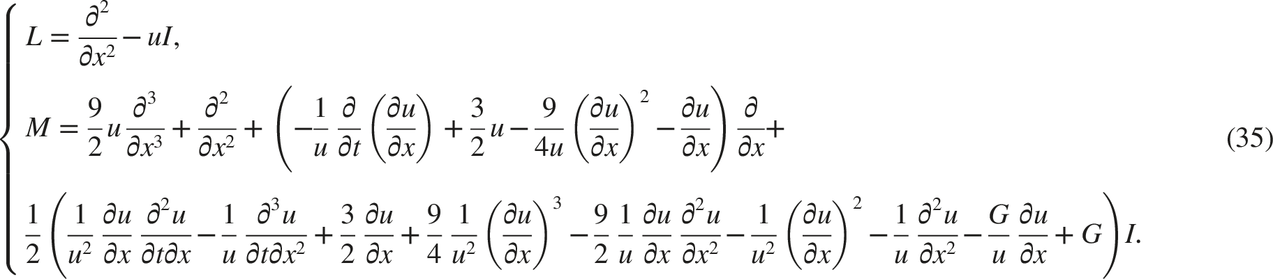
Thus, we have demonstrated that the operators L and M satisfy the Lax equation, implying that the proposed model represents the compatibility condition of the Lax pair given in Eqs. (17) and (18). Solving Eqs. (25) and (26), we obtain the values of l and D as follows:

l = - \frac{G}{3 u},

(31)

where G is the constant of integration.

D = \frac{1}{2} (\frac{\partial C}{\partial x} - \frac{G}{u} \frac{\partial u}{\partial x} + G) .

(32)

Now, let G = −27/2, B = 1 in Eq. (27) via Eq. (31) and integrating the resulting equation (ignoring the constant of integration) we have,

C = - \frac{1}{u} \frac{\partial}{\partial t} (\frac{\partial u}{\partial x}) + \frac{3}{2} u - \frac{9}{4 u} {(\frac{\partial u}{\partial x})}^{2} - \frac{\partial u}{\partial x}

(33)

so, finally we have α, B, C, D as follows,

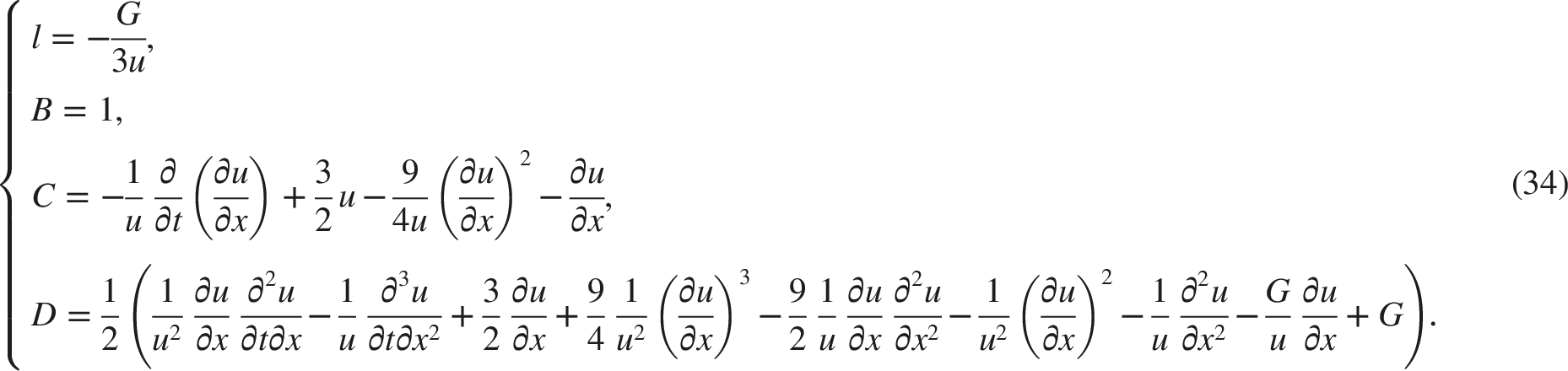
\{\begin{cases} l = - \frac{G}{3 u}, \\ B = 1, \\ C = - \frac{1}{u} \frac{\partial}{\partial t} (\frac{\partial u}{\partial x}) + \frac{3}{2} u - \frac{9}{4 u} {(\frac{\partial u}{\partial x})}^{2} - \frac{\partial u}{\partial x}, \\ D = \frac{1}{2} (\frac{1}{u^{2}} \frac{\partial u}{\partial x} \frac{\partial^{2} u}{\partial t \partial x} - \frac{1}{u} \frac{\partial^{3} u}{\partial t \partial x^{2}} + \frac{3}{2} \frac{\partial u}{\partial x} + \frac{9}{4} \frac{1}{u^{2}} {(\frac{\partial u}{\partial x})}^{3} - \frac{9}{2} \frac{1}{u} \frac{\partial u}{\partial x} \frac{\partial^{2} u}{\partial x^{2}} - \frac{1}{u^{2}} {(\frac{\partial u}{\partial x})}^{2} - \frac{1}{u} \frac{\partial^{2} u}{\partial x^{2}} - \frac{G}{u} \frac{\partial u}{\partial x} + G) . \end{cases}

(34)

Using above values of l, B, C, D in Eq. (17) and Eq. (18), then we obtain the LP as follows,

\{\begin{cases} L = \frac{\partial^{2}}{\partial x^{2}} - u I, \\ M = \frac{9}{2} u \frac{\partial^{3}}{\partial x^{3}} + \frac{\partial^{2}}{\partial x^{2}} + (- \frac{1}{u} \frac{\partial}{\partial t} (\frac{\partial u}{\partial x}) + \frac{3}{2} u - \frac{9}{4 u} {(\frac{\partial u}{\partial x})}^{2} - \frac{\partial u}{\partial x}) \frac{\partial}{\partial x} + \\ \frac{1}{2} (\frac{1}{u^{2}} \frac{\partial u}{\partial x} \frac{\partial^{2} u}{\partial t \partial x} - \frac{1}{u} \frac{\partial^{3} u}{\partial t \partial x^{2}} + \frac{3}{2} \frac{\partial u}{\partial x} + \frac{9}{4} \frac{1}{u^{2}} {(\frac{\partial u}{\partial x})}^{3} - \frac{9}{2} \frac{1}{u} \frac{\partial u}{\partial x} \frac{\partial^{2} u}{\partial x^{2}} - \frac{1}{u^{2}} {(\frac{\partial u}{\partial x})}^{2} - \frac{1}{u} \frac{\partial^{2} u}{\partial x^{2}} - \frac{G}{u} \frac{\partial u}{\partial x} + G) I . \end{cases}

(35)

3. Darboux transformation (DT)

Consider^39–45,54

ψ^{″} (x) + (λ - u) ψ (x) = 0,

(36)

Such a formulation appears frequently in the literature as a Sturm–Liouville problem, where one seeks eigenfunctions and eigenvalues, with u acting as the potential function. In this article, we make use of the Darboux theorem:

3.1. Darboux Theorem

Consider ψ = ψ₁(x) be a solution of SL-problem, for λ = λ₁, suppose the DT,^55,56

ψ [1] = (\frac{d}{d x} - \frac{{ψ_{1}}^{'}}{ψ_{1}}) ψ,

(37)

then (37) holds,

ψ^{″} [1] + (λ - u [1]) ψ [1] = 0, u [1] = u - 2 \frac{d}{d x} (\frac{{ψ_{1}}^{'}}{ψ_{1}}) .

(38)

3.2. DT for Eq. (2)

To this concern, Eq. (30) can be assumed as,(2)

L ψ = λ ψ,

(39)

ψ_{t} = M ψ .

(40)

subject to the consistency condition:

[\frac{\partial L}{\partial t} + [L, M]] ψ = 0

(41)

while Eq. (39) and Eq. (40) is covariant under the DT hence,

L [1] ψ [1] = λ ψ [1],

(42)

ψ_{t} [1] = M [1] ψ [1],

(43)

and the consistency condition becomes as,

\frac{\partial u [1]}{\partial t} - \frac{\partial}{\partial t} (\frac{\partial^{2} u [1]}{\partial x^{2}}) + \frac{3}{2} u [1] \frac{\partial u [1]}{\partial x} - \frac{9}{2} \frac{\partial u [1]}{\partial x} \frac{\partial^{2} u [1]}{\partial x^{2}} - \frac{9}{2} u [1] \frac{\partial^{3} u [1]}{\partial x^{3}} = 0,

(44)

This implies that u¹ is a new solution of Eq. (2), which can be obtained from the original unknown solution u.

4. Single-soliton solution via darboux transformation

Using Eq. (35), Eq. (39) and Eq. (40),^39–45,54

\frac{\partial^{2} ψ}{\partial x^{2}} - u ψ = λ ψ,

(45)

\begin{matrix} \frac{\partial ψ}{\partial t} - \frac{9}{2} u \frac{\partial^{3} ψ}{\partial x^{3}} - \frac{\partial^{2} ψ}{\partial x^{2}} - (- \frac{1}{u} \frac{\partial}{\partial t} (\frac{\partial u}{\partial x}) + \frac{3}{2} u - \frac{9}{4 u} {(\frac{\partial u}{\partial x})}^{2} - \frac{\partial u}{\partial x}) \frac{\partial ψ}{\partial x} - \\ \frac{1}{2} (\frac{1}{u^{2}} \frac{\partial u}{\partial x} \frac{\partial^{2} u}{\partial t \partial x} - \frac{1}{u} \frac{\partial^{3} u}{\partial t \partial x^{2}} + \frac{3}{2} \frac{\partial u}{\partial x} + \frac{9}{4} \frac{1}{u^{2}} {(\frac{\partial u}{\partial x})}^{3} - \frac{9}{2} \frac{1}{u} \frac{\partial u}{\partial x} \frac{\partial^{2} u}{\partial x^{2}} - \frac{1}{u^{2}} {(\frac{\partial u}{\partial x})}^{2} - \frac{1}{u} \frac{\partial^{2} u}{\partial x^{2}} - \frac{G}{u} \frac{\partial u}{\partial x} + G) ψ = 0 . \end{matrix}

(46)

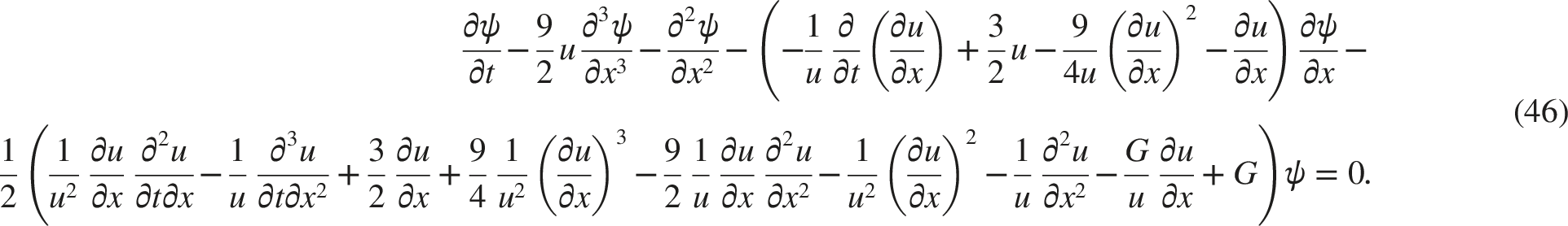
Via DT on ψ,

ψ [1] = (\frac{d}{d x} - \frac{{ψ_{1}}^{'}}{ψ_{1}}), ψ_{1} = ψ_{1} (x, t) .

(47)

Then the system in Eq. (45) and Eq. (46) is covariant under the DT, then

\frac{\partial^{2} ψ [1]}{\partial x^{2}} - u [1] ψ [1] = λ ψ [1]

(48)

\begin{matrix} \frac{\partial ψ [1]}{\partial t} - \frac{9}{2} u [1] \frac{\partial^{3} ψ [1]}{\partial x^{3}} - \frac{\partial^{2} ψ [1]}{\partial x^{2}} - (- \frac{1}{u [1]} \frac{\partial}{\partial t} (\frac{\partial u [1]}{\partial x}) + \frac{3}{2} u [1] - \frac{9}{4 u [1]} {(\frac{\partial u [1]}{\partial x})}^{2} - \frac{\partial u [1]}{\partial x}) \frac{\partial ψ [1]}{\partial x} - \\ \frac{1}{2} (\frac{1}{u^{2} [1]} \frac{\partial u [1]}{\partial x} \frac{\partial^{2} u [1]}{\partial t \partial x} - \frac{1}{u [1]} \frac{\partial^{3} u [1]}{\partial t \partial x^{2}} + \frac{3}{2} \frac{\partial u [1]}{\partial x} + \frac{9}{4} \frac{1}{u^{2} [1]} {(\frac{\partial u [1]}{\partial x})}^{3} - Ω) ψ [1] = 0, \end{matrix}

(49)

where

Ω = 9 / 21 / u [1] \partial u [1] / \partial x \partial^{2} u [1] / \partial x^{2} - 1 / u^{2} [1] {(\partial u [1] / \partial x)}^{2} - 1 / u [1] \partial^{2} u [1] / \partial x^{2} - G / u [1] \partial u [1] / \partial x + G

and

u [1] = u - 2 {ψ_{1}}^{'} / ψ_{1}

is a new exact solution for Eq. (2) and u will be the initial solution (i.e u = 0) and substituting this vale in Eq.(45) and Eq.(46), we have

\frac{\partial^{2} ψ}{\partial x^{2}} - λ ψ = 0,

(50)

\frac{\partial ψ}{\partial t} + \frac{\partial^{2} ψ}{\partial x^{2}} - \frac{G}{2} ψ = 0 .

(51)

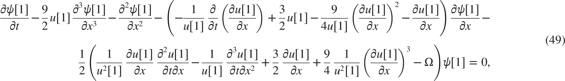
λ = k², we lett A(t)exp(kx) be the solution of Eq. (50), Eq. (51) and integrating it,

A (t) = e x p [(\frac{G - 2 k^{2}}{2}) t - k x_{0}],

(52)

where kx₀ is constant of integration. Therefore,

ψ^{1} = e x p [k x - (\frac{G - 2 k^{2}}{2}) t - k x_{0}],

(53)

ψ¹ is the solution of Eq. (50) and Eq. (51). Also,

ψ^{2} = e x p [- k x - (\frac{G - 2 k^{2}}{2}) t - k x_{0}],

(54)

ψ² is the solution of Eq. (50) and Eq. (51), so there general solution will be

ψ = c_{1} e x p [k x - (\frac{G - 2 k^{2}}{2}) t - k x_{0}] + c_{2} e x p [- k x - (\frac{G - 2 k^{2}}{2}) t - k x_{0}] .

(55)

Now setting c₁ = 1/2, c₂ = 1/2, then we have

ψ_{1} = \cosh [k x - (\frac{G - 2 k^{2}}{2}) t - k x_{0}] .

(56)

If we set c₁ = 1/2, c₂ = −1/2, then we have

ψ_{2} = \sinh [k x - (\frac{G - 2 k^{2}}{2}) t - k x_{0}] .

(57)

Inserting Eq. (55) in Eq. (47) we have,

ψ [1] = [\frac{d}{d x} - \tanh [k x - (\frac{G - 2 k^{2}}{2}) t - k x_{0}]] ψ .

(58)

then

u [1] = - 2 k^{2} \sec h^{2} [k x - (\frac{G - 2 k^{2}}{2}) t - k x_{0}] .

(59)

Now, put $k = \sqrt{λ}$ in above equation,

u [1] = - 2 λ \sec h^{2} [\sqrt{λ} x - (\frac{G - 2 λ}{2}) t - \sqrt{λ} x_{0}],

(60)

where u¹ is the required solution.

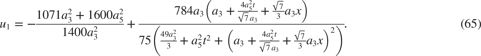
5. Lump solutions (LS)

For LS of Eq. (2), we use,^57,58

u (x, t) = 2 b {(\ln f)}_{x} + m,

(61)

and get the following

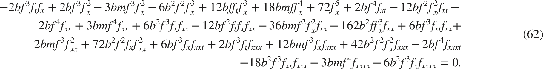
\begin{matrix} - 2 b f^{3} f_{t} f_{x} + 2 b f^{3} f_{x}^{2} - 3 b m f^{3} f_{x}^{2} - 6 b^{2} f^{2} f_{x}^{3} + 12 b f f_{t} f_{x}^{3} + 18 b m f f_{x}^{4} + 72 f_{x}^{5} + 2 b f^{4} f_{x t} - 12 b f^{2} f_{x}^{2} f_{x t} - \\ 2 b f^{4} f_{x x} + 3 b m f^{4} f_{x x} + 6 b^{2} f^{3} f_{x} f_{x x} - 12 b f^{2} f_{t} f_{x} f_{x x} - 36 b m f^{2} f_{x}^{2} f_{x x} - 162 b^{2} f f_{x}^{3} f_{x x} + 6 b f^{3} f_{x t} f_{x x} + \\ 2 b m f^{3} f_{x x}^{2} + 72 b^{2} f^{2} f_{x} f_{x x}^{2} + 6 b f^{3} f_{x} f_{xxt} + 2 b f^{3} f_{t} f_{xxx} + 12 b m f^{3} f_{x} f_{xxx} + 42 b^{2} f^{2} f_{x}^{2} f_{xxx} - 2 b f^{4} f_{xxxt} \\ - 18 b^{2} f^{3} f_{x x} f_{xxx} - 3 b m f^{4} f_{xxxx} - 6 b^{2} f^{3} f_{x} f_{xxxx} = 0 . \end{matrix}

(62)

Now f in Eq. (62) can be taken as,^57,58

f = ϒ_{1}^{2} + ϒ_{2}^{2} + a_{7},

(63)

where ϒ₁ = a₁x + a₂t + a₃, ϒ₂ = a₄x + a₅t + a₆, a_i(1 ≤ i ≤ 7) are constants. Usage of f into Eq. (62) and determining the coefficients of x and t yields:

Set I. If a₄ = a₆ = 0

a_{1} = \frac{\sqrt{7} a_{3}}{3}, a_{2} = \frac{4 a_{5}^{2} \sqrt{7}}{7 a_{3}}, a_{7} = \frac{49 a_{3}^{2}}{3}, b = \frac{28 \sqrt{7}}{25}, m = - \frac{1071 a_{3}^{2} + 1600 a_{5}^{2}}{1400 a_{3}^{2}} .

(64)

These parameters generates the LS

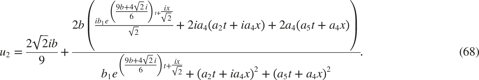
u_{1} = - \frac{1071 a_{3}^{2} + 1600 a_{5}^{2}}{1400 a_{3}^{2}} + \frac{784 a_{3} (a_{3} + \frac{4 a_{5}^{2} t}{\sqrt{7} a_{3}} + \frac{\sqrt{7}}{3} a_{3} x)}{75 (\frac{49 a_{3}^{2}}{3} + a_{5}^{2} t^{2} + {(a_{3} + \frac{4 a_{5}^{2} t}{\sqrt{7} a_{3}} + \frac{\sqrt{7}}{3} a_{3} x)}^{2})} .

(65)

6. Lump with 1-strip solution (L1S)

To get L1S, we use the transformation,⁴⁹

f = ϒ_{1}^{2} + ϒ_{2}^{2} + a_{7} + b_{1} e^{k_{1} x + k_{2} t},

(66)

where ϒ₁ = a₁x + a₂t + a₃, ϒ₂ = a₄x + a₅t + a₆, a_i(1 ≤ i ≤ 7), k₁, k₂ and b₁ are constants. Application of f in Eq. (62) and determining the coefficients of exp-functions, x and t yields:

Set I. When a₃ = a₆ = 0,

a_{1} = \sqrt{- 1} a_{4}, k_{1} = \frac{\sqrt{2} i}{2}, k_{2} = \frac{9 b + 4 \sqrt{2} i}{6}, m = \frac{2 \sqrt{- 2} b}{9}, a_{7} = 0 .

(67)

These values exhibits the required solution,

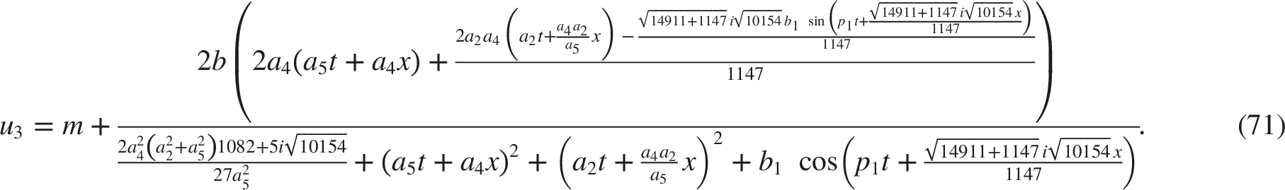
u_{2} = \frac{2 \sqrt{2} i b}{9} + \frac{2 b (\frac{i b_{1} e^{(\frac{9 b + 4 \sqrt{2} i}{6}) t + \frac{i x}{\sqrt{2}}}}{\sqrt{2}} + 2 i a_{4} (a_{2} t + i a_{4} x) + 2 a_{4} (a_{5} t + a_{4} x))}{b_{1} e^{(\frac{9 b + 4 \sqrt{2} i}{6}) t + \frac{i x}{\sqrt{2}}} + {(a_{2} t + i a_{4} x)}^{2} + {(a_{5} t + a_{4} x)}^{2}} .

(68)

7. Lump periodic (LP)

To get LP, we apply the transformation,⁴⁹

f = ϒ_{1}^{2} + ϒ_{2}^{2} + a_{7} + b_{1} \cos (k_{1} x + p_{1} t),

(69)

where ϒ₁ = a₁x + a₂t + a₃, ϒ₂ = a₄x + a₅t + a₆, a_i(1 ≤ i ≤ 7), k₁, b₁ and p₁ are distinct values to determined. Inserting f in Eq. (62) and determining the coefficients of the cos function, x and t yields:

Set I. If a₃ = a₆ = 0,

a_{1} = \frac{a_{4} a_{2}}{a_{5}}, k_{1} = \frac{\sqrt{14911 + 1147} i \sqrt{10154}}{1147}, a_{7} = \frac{2 a_{4}^{2} (a_{2}^{2} + a_{5}^{2}) 1082 + 5 i \sqrt{10154}}{27 a_{5}^{2}}, a_{2} = a_{2}, a_{5} = a_{5}, m = m .

(70)

then

u_{3} = m + \frac{2 b (2 a_{4} (a_{5} t + a_{4} x) + \frac{2 a_{2} a_{4} (a_{2} t + \frac{a_{4} a_{2}}{a_{5}} x) - \frac{\sqrt{14911 + 1147} i \sqrt{10154} b_{1} \sin (p_{1} t + \frac{\sqrt{14911 + 1147} i \sqrt{10154} x}{1147})}{1147}}{1147})}{\frac{2 a_{4}^{2} (a_{2}^{2} + a_{5}^{2}) 1082 + 5 i \sqrt{10154}}{27 a_{5}^{2}} + {(a_{5} t + a_{4} x)}^{2} + {(a_{2} t + \frac{a_{4} a_{2}}{a_{5}} x)}^{2} + b_{1} \cos (p_{1} t + \frac{\sqrt{14911 + 1147} i \sqrt{10154} x}{1147})} .

(71)

8. Rouge wave solutions (RWs)

To obtain the RWS, we employ the transformation provided in Eq. (4),⁵⁹

f = ϒ_{1}^{2} + ϒ_{2}^{2} + b_{1} \cosh (k_{1} z + p_{1} t) + a_{7},

(72)

where ϒ₁ = a₁x + a₂t + a₃, ϒ₂ = a₄x + a₅t + a₆.

The parameters a_i (1 ≤ i ≤ 7), along with k₁, p₁, and b₁, are assumed to be arbitrary real constants. By substituting the function f into Eq. (62) and setting the coefficients of the hyperbolic terms, as well as those of x and t, to zero, we solve the resulting algebraic equations and obtain:

Set I. When a₃ = a₆ = 0,

a_{7} = \frac{16 a_{1}^{2} (a_{2}^{2} + a_{5}^{2})}{a_{5}^{2}}, a_{4} = - \frac{a_{1} a_{2}}{a_{5}}, k_{1} = \frac{\sqrt{2}}{2}, a_{2} = a_{2} .

(73)

These parameters gives the RWS,

u_{4} = m + \frac{2 b (2 a_{4} (a_{5} t + a_{4} x) - \frac{2 a_{2} a_{4} (a_{2} t + \frac{a_{4} a_{2} x}{a_{5}})}{a_{5}} + \frac{b_{1} \sinh (p_{1} t + \frac{x}{\sqrt{2}})}{\sqrt{2}})}{\frac{16 a_{1}^{2} (a_{2}^{2} + a_{5}^{2})}{a_{5}^{2}} + {(a_{5} t + a_{4} x)}^{2} + {(a_{2} t + \frac{a_{4} a_{2} x}{a_{5}})}^{2} + b_{1} \cosh (p_{1} t + \frac{x}{\sqrt{2}})} .

(74)

9. Manifold periodic solution (MPS)

To get MPS, we consider f as,⁶⁰

f = e^{- d_{1} ϒ_{1}} + h_{1} e^{d_{1} ϒ_{1}} + h_{2} \cos (d_{2} ϒ_{2}),

(75)

where ϒ₁ = a₁x + a₂t + a₃, ϒ₂ = a₄x + a₅t + a₆.

The quantities a_i (1 ≤ i ≤ 6), h₁, h₂, and d₁ are parameters to be determined. By inserting f into Eq. (62) and equating the coefficients of cos(⋅), x, and t to zero, we arrive at the following results:

Set I. When

\{\begin{cases} b = - \frac{12 a_{1}^{4} d_{1}^{4} m + 8 a_{1}^{3} a_{2} d_{1}^{4} - 3 a_{1}^{2} d_{1}^{2} m + 2 a_{1}^{2} d_{1}^{2} - 2 a_{1} a_{2} d_{1}^{2} - 1}{6 a_{1}^{3} d_{1}^{3} (4 a_{1}^{2} d_{1}^{2} - 1)}, \\ a_{4} = \frac{480 a_{1}^{8} d_{1}^{8} m + 320 a_{1}^{7} a_{2} d_{1}^{8} - 600 a_{1}^{6} d_{1}^{6} m + 32 a_{1}^{6} d_{1}^{6} - 472 a_{1}^{5} a_{2} d_{1}^{6} + Φ}{6 a_{1}^{2} d_{1}^{2} (4 a_{1}^{2} d_{1}^{2} - 1) d_{2} \sqrt{3 a_{1}^{2} d_{1}^{2} - 1}}, \\ Φ = 228 a_{1}^{4} d_{1}^{4} m - 100 a_{1}^{4} d_{1}^{4} + 194 a_{1}^{3} a_{2} d_{1}^{4} - 27 a_{1}^{2} d_{1}^{2} m + 65 a_{1}^{2} d_{1}^{2} - 24 a_{1} a_{2} d_{1}^{2} - 12, \\ a_{5} = \frac{\sqrt{3 a_{1}^{2} d_{1}^{2} - 1}}{d_{2}}, \\ h_{1} = 0 . \end{cases}

(76)

These values exhibits the MPS,

\begin{aligned} u_{5} = & m - \frac{e^{d_{1} (a_{3} + a_{2} t + a_{1} x)} A}{3 a_{1}^{3} d_{1}^{3} (1 - 4 a_{1}^{2} d_{1}^{2})} \\ \times [- a_{1} d_{1} e^{- d_{1} (a_{3} + a_{2} t + a_{1} x)} \\ - \frac{h_{2} B}{6 a_{1}^{2} d_{1}^{2} \sqrt{- 1 + 3 a_{1}^{2} d_{1}^{2}} (1 - 4 a_{1}^{2} d_{1}^{2})} \\ \times \sin (a_{6} d_{2} + \sqrt{- 1 + 3 a_{1}^{2} d_{1}^{2}} t + \frac{B x}{6 a_{1}^{2} d_{1}^{2} \sqrt{- 1 + 3 a_{1}^{2} d_{1}^{2}} (1 - 4 a_{1}^{2} d_{1}^{2})})] \\ \times \frac{1}{1 + e^{d_{1} (a_{3} + a_{2} t + a_{1} x)} h_{2} \cos (a_{6} d_{2} + \sqrt{- 1 + 3 a_{1}^{2} d_{1}^{2}} t + \frac{B x}{6 a_{1}^{2} d_{1}^{2} \sqrt{- 1 + 3 a_{1}^{2} d_{1}^{2}} (1 - 4 a_{1}^{2} d_{1}^{2})})}, \end{aligned}

(77)

where

A = - 1 - 2 a_{1} a_{2} d_{1}^{2} + 8 a_{1}^{3} a_{2} d_{1}^{4} + a_{1}^{2} d_{1}^{2} (2 - 3 m) + 12 a_{1}^{4} d_{1}^{4} m

, and

B = - 12 - 24 a_{1} a_{2} d_{1}^{2} + 194 a_{1}^{3} a_{2} d_{1}^{4} - 472 a_{1}^{5} a_{2} d_{1}^{6} + 320 a_{1}^{7} a_{2} d_{1}^{8} + a_{1}^{2} d_{1}^{2} (65 - 27 m) + 480 a_{1}^{8} d_{1}^{8} m + 4 a_{1}^{4} d_{1}^{4} (- 25 + 57 m) - 8 a_{1}^{6} d_{1}^{6} (- 4 + 75 m)

10. Ma-breathers (MBs) and its relating rouge wave

For obtaining MBs, we assume f in the form,61

f = a_{1} + e^{i (p_{1} x)} + e^{- i (p_{1} x)} e^{k_{1} t + k_{2}} + b_{1} e^{2 (k_{1} t + k_{2})},

(78)

where a₁, p₁, k₁, k₂ are any parameters. Now, utilizing f in Eq.(62) and taking the coefficients of exp, x, t functions to zero and after solving these equations we get:

Set I. When

m = - \frac{(\frac{2 i}{3}) (44 b p_{1}^{3} - b p_{1} + i)}{(2 p_{1} - 1) (2 p_{1} + 1)}, b_{1} = 0, p_{1} = p_{1}, a_{2} = a_{2}, b_{2} = b_{2} .

(79)

These values forms MB,

u_{6} = - \frac{(\frac{2 i}{3}) (44 b p_{1}^{3} - b p_{1} + i)}{(2 p_{1} - 1) (2 p_{1} + 1)} + \frac{2 b (- i e^{- i p_{1} x} p_{1} + i e^{i p_{1} x} p_{1})}{e^{- i p_{1} x} + e^{- i p_{1} x}} .

(80)

11. Kuznetsov–Ma breather (KMB) and its relating rouge wave

We use, f as follows,⁶¹

f = e^{- p_{1} (x - b_{1} t)} + a_{1} \cos (p (x + b_{1} t)) + a_{2} \cos (p (x - b_{1} t)),

(81)

where p_i, b_i and a_i are constant. Usage of f in Eq.(58) and determining the coefficients of exp and cos functions yields:

Set I

b_{1} = - \frac{6 p_{1} (64 b p_{1}^{4} - 20 b p_{1}^{2} + b + 4 p_{1})}{{(4 p_{1}^{2} - 1)}^{2}}, p = i p_{1}, m = \frac{2 (12 b p_{1}^{3} - 3 b p_{1} - 1)}{3 (4 p_{1}^{2} - 1)}, a_{2} = 0, a_{3} = a_{3} .

(82)

These parameters forms proposed solution,

\begin{aligned} u_{7} = & \frac{2 (12 b p_{1}^{3} - 3 b p_{1} - 1)}{3 (4 p_{1}^{2} - 1)} \\ + \frac{2 b}{e^{- p_{1} (- \frac{6 p_{1} (64 b p_{1}^{4} - 20 b p_{1}^{2} + b + 4 p_{1}) t}{{(4 p_{1}^{2} - 1)}^{2}} + x)} + a_{1} \cosh (p_{1} (- \frac{6 p_{1} (64 b p_{1}^{4} - 20 b p_{1}^{2} + b + 4 p_{1}) t}{{(4 p_{1}^{2} - 1)}^{2}} + x))} \\ \times (- \frac{e^{- p_{1} (- \frac{6 p_{1} (64 b p_{1}^{4} - 20 b p_{1}^{2} + b + 4 p_{1}) t}{{(4 p_{1}^{2} - 1)}^{2}} + x)}}{p_{1}} + a_{1} p_{1} \sinh (p_{1} (- \frac{6 p_{1} (64 b p_{1}^{4} - 20 b p_{1}^{2} + b + 4 p_{1}) t}{{(4 p_{1}^{2} - 1)}^{2}} + x))) . \end{aligned}

(83)

12. Generalized breather (GBs)

In order to get GBs, we will use ansatz,⁶²

u (x, t) = 2 b c {(\frac{6}{k} \ln ϕ (x, t))}_{x} + n, u = u (x, t),

(84)

where n, k, b and c are constants and Eq. (84), Eq. (2),

\begin{matrix} - 12 b c k ϕ^{3} ϕ_{t} ϕ_{x} + 12 b c k ϕ^{3} ϕ_{x}^{2} - 18 b c k ϕ^{3} ϕ_{x}^{2} - 216 b^{2} c^{2} ϕ^{2} ϕ_{x}^{3} + 72 b c k ϕ ϕ_{t} ϕ_{x}^{3} + 108 b c k m ϕ ϕ_{x}^{4} + 2592 b^{2} c^{2} ϕ_{x}^{5} + \\ 12 b c k ϕ^{4} ϕ_{x t} - 72 b c k ϕ^{2} ϕ_{x}^{2} ϕ_{x t} - 12 b c k ϕ^{4} ϕ_{x x} + 18 b c k m ϕ^{4} ϕ_{x x} + 216 b^{2} c^{2} ϕ^{3} ϕ_{x} ϕ_{x x} - 72 b c k ϕ^{2} ϕ_{t} ϕ_{x} ϕ_{x x} - \\ 216 b c k m ϕ^{2} ϕ_{x}^{2} ϕ_{x x} - 5832 b^{2} c^{2} ϕ ϕ_{x}^{3} ϕ_{x x} + 36 b c k ϕ^{3} ϕ_{x t} ϕ_{x x} + 54 b c k m ϕ^{3} ϕ_{x x}^{2} + 2592 b^{2} c^{2} ϕ^{2} ϕ_{x} ϕ_{x x}^{2} + \\ 36 b c k ϕ^{3} ϕ_{x} ϕ_{xxt} + 12 b c k ϕ^{3} ϕ_{t} ϕ_{xxx} + 72 b c k m ϕ^{3} ϕ_{x} ϕ_{xxx} + 1512 b^{2} c^{2} ϕ^{2} ϕ_{x}^{2} ϕ_{xxx} - 648 b^{2} c^{2} ϕ^{3} ϕ_{x x} ϕ_{xxx} - \\ 12 b c k ϕ^{4} ϕ_{xxxt} - 18 b c k m ϕ^{4} ϕ_{xxxx} - 216 b^{2} c^{2} ϕ^{3} ϕ_{x} ϕ_{xxxx} = 0 \end{matrix}

(85)

For GB, we use ϕ in Eq. (85),

ϕ = \frac{(1 - 4 c) \cosh (σ t) + \sqrt{2 c} \cos (ρ x) + i σ \sinh (σ t)}{\sqrt{2 c} \cos (ρ x) - \cosh (σ t)} e^{i t},

(86)

The constants ρ, σ, and c are to be identified. Upon equating the coefficients of sinh, cosh, and exp terms to zero, the solution yields the following:

Set I

c = \frac{1}{2}, n = n, ρ = \frac{1}{2} + \frac{i}{2} \sqrt{3}, σ = σ, b = b .

(87)

These values makes GB to Eq. (1),

u_{8} = n + \frac{6 b e^{- i t} (\cos (\frac{1 + i \sqrt{3}}{2}) x) - \cosh (t σ) (Π + \frac{(\frac{1 + i \sqrt{3}}{2}) e^{i t} s i n ((\frac{1 + i \sqrt{3}}{2}) x) \cos ((\frac{1 + i \sqrt{3}}{2}) x) - \cosh (t σ) + i σ \sinh (t σ)}{{(\cos ((\frac{1 + i \sqrt{3}}{2}) x) - \cosh (t σ))}^{2}})}{k (\cos ((\frac{1 + i \sqrt{3}}{2}) x) - \cosh (t σ) + i σ \sinh (t σ))},

(88)

where

Π = (\frac{1 + i \sqrt{3}}{2}) e^{i t} s i n ((\frac{1 + i \sqrt{3}}{2}) x) / \cos ((\frac{1 + i \sqrt{3}}{2}) x) - \cosh (t σ)

13. Akhmediev breathers (ABs)

We assume ψ as follows,⁶³

ψ = \sqrt{p_{0}} \frac{(1 - 4 a) \cosh (b x) + i b \sinh (b x) + \sqrt{2 a} \cos (ω_{\mod} T)}{\sqrt{2 a} \cos (ω_{\mod} T) - \cosh (b x)},

(89)

where ω_mod stands for perturbation frequency (PF) with p₀ as the power, while a, b are given by b = [8a(1 − 2a)]²,

2 a = 1 - {(ω_{\mod} / ω_{c})}^{2}

and

ω_{c}^{2} = 4 p_{0} γ / | β_{2} |

Equating the coefficients of trigonometric and hyperbolic terms to zero and solving yields:

Set I. When

a = \frac{1}{2}, b = - \sqrt{\frac{2 - 3 n}{12 n}}, c = - \frac{144 i k n^{3} (\sqrt{\frac{2 - 3 n}{12 n}})}{(3 n - 2) (153 n - 14)}, ρ = ρ, p_{0} = p_{0} .

(90)

therefore ABs,

u_{9} = n + \frac{144 i k n^{2} (2 - 3 n) (\cos (t ω) - \cosh (\frac{\sqrt{\frac{2 - 3 n}{2 n}} x}{2 \sqrt{3}})) (\frac{\sqrt{p_{0}} (\frac{i (2 - 3 n) \cosh (\frac{\sqrt{\frac{2 - 3 n}{2 n}} x}{2 \sqrt{3}})}{12 n} - \frac{\sqrt{\frac{2 - 3 n}{2 n}} s i n h (\frac{\sqrt{\frac{2 - 3 n}{2 n}} x}{2 \sqrt{3}})}{2 \sqrt{3}})}{\cos (t ω) - \cosh (\frac{\sqrt{\frac{2 - 3 n}{2 n}} x}{2 \sqrt{3}})} + Π_{1})}{(3 n - 2) (153 n - 14) (\cos (t ω) - \cosh (\frac{\sqrt{\frac{2 - 3 n}{2 n}} x}{2 \sqrt{3}}) + \frac{i \sqrt{\frac{2 - 3 n}{2 n}} s i n h (\frac{\sqrt{\frac{2 - 3 n}{2 n}} x}{2 \sqrt{3}})}{2 \sqrt{3}})},

(91)

where

Π_{1} = \sqrt{\frac{2 - 3 n}{2 n}} \sqrt{p_{0}} s i n h (\frac{\sqrt{\frac{2 - 3 n}{2 n}} x}{2 \sqrt{3}}) (\cos (t ω) - \cosh (\frac{\sqrt{\frac{2 - 3 n}{2 n}} x}{2 \sqrt{3}}) + \frac{i \sqrt{\frac{2 - 3 n}{2 n}} s i n h (\frac{\sqrt{\frac{2 - 3 n}{2 n}} x}{2 \sqrt{3}})}{2 \sqrt{3}}) / {(\cos (t ω) - \cosh (\frac{\sqrt{\frac{2 - 3 n}{2 n}} x}{2 \sqrt{3}}))}^{2}

14. Result and discussions

Many researchers solved the prosed model particularly, Li et al. studied the entropy weak solution to a gFW-equation,⁴⁸ Camacho et al. worked on symmetries and conservation for proposed model,⁴⁶ Dai et al. evaluated the classifications and representation of single wave solutions to the gFW-equation.⁴⁹ and Itasaka studied Wave-breaking phenomena to gFW-equation,⁴⁷ Abidi et al. evaluated exact solutions for stated model via homotopy analysis and Adomian’s decomposition schemes,⁶⁴ Manafian et al. studied the modified gFW-equation for classification of the single traveling wave solutions,⁶⁵ Wei et al. evaluated wave breaking analysis for FW-equation,⁶⁶ Hormann et al. presented well-posedness,solution concepts for FW-equation.⁶⁷ and Ahmad et al. worked on numerical solutions for FW-equation.⁶⁸ But here in this work, we construct, for the first time, a systematic framework combining the Lax pair structure with the Darboux transformation for the gFW-equation, which has not been fully explored in the existing literature. We derive a wide spectrum of exact solutions within a unified analytical setting, including lump solutions, lump–1-strip, lump–periodic, manifold periodic waves, and multiple types of breather and rogue wave structures via choosing appropriate transformations and symbolic computation. The coexistence and interaction of these solutions in the gFW-system represent a novel contribution. We provide explicit constructions of higher-order and hybrid wave structures (such as lump–periodic and lump–stripe interactions), which reveal new dynamical behaviors not previously reported for this model. The study establishes connections between different classes of nonlinear waves (e.g., Ma breather, Akhmediev breather, and rogue waves) within the same mathematical framework, offering new insight into energy localization and transition mechanisms. Compared to existing studies that focus on isolated solution types, our work presents a comprehensive analysis of multiple nonlinear structures and their interactions, enhancing the understanding of complex wave dynamics.^69–75

The exact solutions obtained in this work such as lump waves, breather structures, periodic waves, and rogue waves have clear physical interpretations. Lump solutions describe highly localized wave packets that can model energy concentration in fluids and optical media. Breather solutions (including Ma, Kuznetsov–Ma, and Akhmediev breathers) represent oscillatory modes that capture modulation instability and recurrence phenomena observed in optical fibers and water wave tanks. Rogue wave solutions, characterized by their sudden and extreme amplitude, are particularly relevant for understanding hazardous ocean waves and high intensity pulses in nonlinear optics. Moreover, the interaction structures such as lump–periodic and lump–stripe waves provide insight into complex wave superposition and energy exchange mechanisms, which are essential for predicting nonlinear wave evolution in realistic environments. From a practical perspective, these analytical solutions serve as benchmark models for validating numerical simulations and experimental observations. They also contribute to the prediction and potential control of extreme events, such as rogue waves in oceanography and signal amplification in fiber optics.

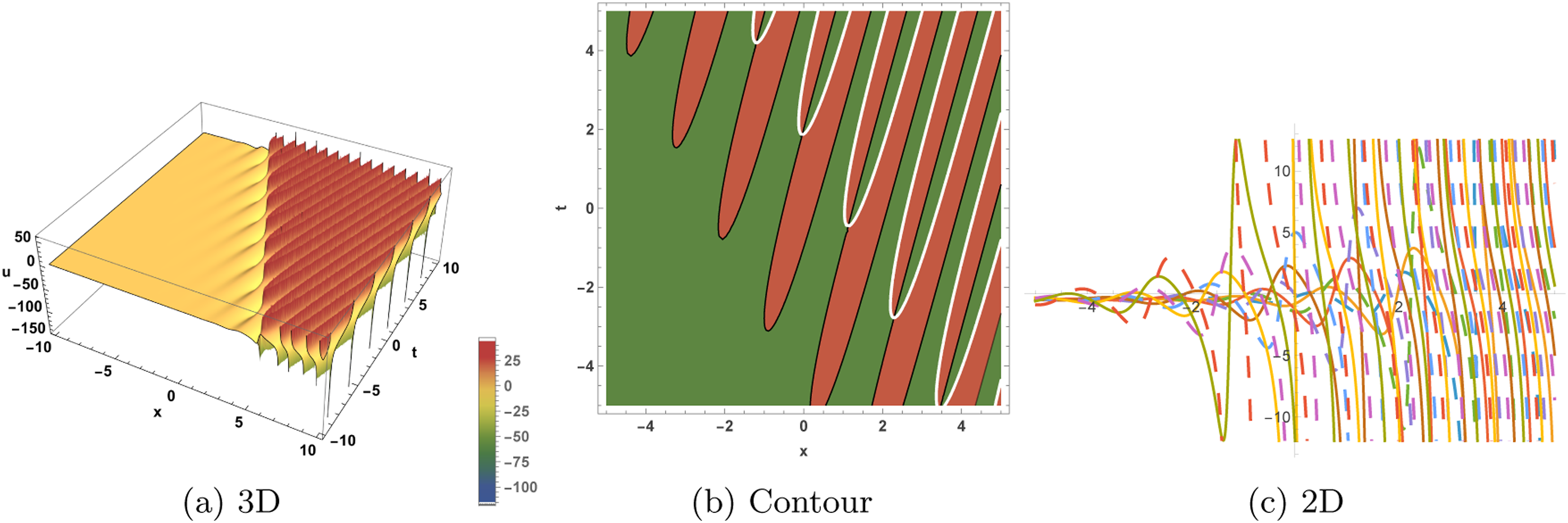
Figure 1 shows the 3D profiles for one-soliton solution in Eq. (60) by using the values of G = 2, x₀ = 3. (a) Representing the 3D plots at λ = −10, (b) at λ = 0.1, and (c) and at λ = 10, respectively. Figure 2 depicts behaviour of the lump–stripe (LS) solution (Eq. (65)) for a₃ = 2 under varying a₅. (a) a₅ = −15: weak lump on stripe background; (b) a₅ = −10: enhanced lump–stripe interaction; (c) a₅ = −5: localized peak intensifies; (d) a₅ = 0: transition to asymmetric profile; (e) a₅ = 5: oscillatory lump–stripe structure; (f) a₅ = 10: stabilized localized peak; (g) a₅ = −15: elongated contour along stripe; (h) a₅ = −10: compressed elliptical structure; (i) a₅ = −5: rotated localized contours; (j) a₅ = 0: vertical stripe dominance; (k) a₅ = 5: tilted lump formation; (l) a₅ = 10: stretched and shifted contours. Figure 3 represents evolution of the lump with stripe solution for different values of a₂. (a) a₂ = −15: weak lump attached to stripe; (b) a₂ = −10: interaction strengthens near interface; (c) a₂ = −5: localized peak develops; (d) a₂ = 0.5: localized peak develops; (e) a₂ = 5: pronounced lump on stripe; (f) a₂ = 10: shifted and stabilized structure; (g) a₂ = −15: shallow contour with small depression; (h) a₂ = −10: symmetric localized contours; (i) a₂ = −5: asymmetric spreading pattern; (j) a₂ = 0.5: localized peak develops; (k) a₂ = 5: compact lump beneath stripe; (l) a₂ = 10: extended interaction region.

Figure 1.

The 3D profiles for one-soliton solution in Eq. (60) are formed with the values of G = 2, x₀ = 3. (a) Representing the 3D plots at λ = −10, (b) at λ = 0.1, and (c) and at λ = 10, respectively.

Figure 2.

Behaviour of the lump–stripe (LS) solution (Eq. (65)) for a₃ = 2 under varying a₅. (a) a₅ = −15: weak lump on stripe background; (b) a₅ = −10: enhanced lump–stripe interaction; (c) a₅ = −5: localized peak intensifies; (d) a₅ = 0: transition to asymmetric profile; (e) a₅ = 5: oscillatory lump–stripe structure; (f) a₅ = 10: stabilized localized peak; (g) a₅ = −15: elongated contour along stripe; (h) a₅ = −10: compressed elliptical structure; (i) a₅ = −5: rotated localized contours; (j) a₅ = 0: vertical stripe dominance; (k) a₅ = 5: tilted lump formation; (l) a₅ = 10: stretched and shifted contours.

Figure 3.

Evolution of the lump with stripe solution for different values of a₂. (a) a₂ = −15: weak lump attached to stripe; (b) a₂ = −10: interaction strengthens near interface; (c) a₂ = −5: localized peak develops; (d) a₂ = 0.5: localized peak develops; (e) a₂ = 5: pronounced lump on stripe; (f) a₂ = 10: shifted and stabilized structure; (g) a₂ = −15: shallow contour with small depression; (h) a₂ = −10: symmetric localized contours; (i) a₂ = −5: asymmetric spreading pattern; (j) a₂ = 0.5: localized peak develops; (k) a₂ = 5: compact lump beneath stripe; (l) a₂ = 10: extended interaction region.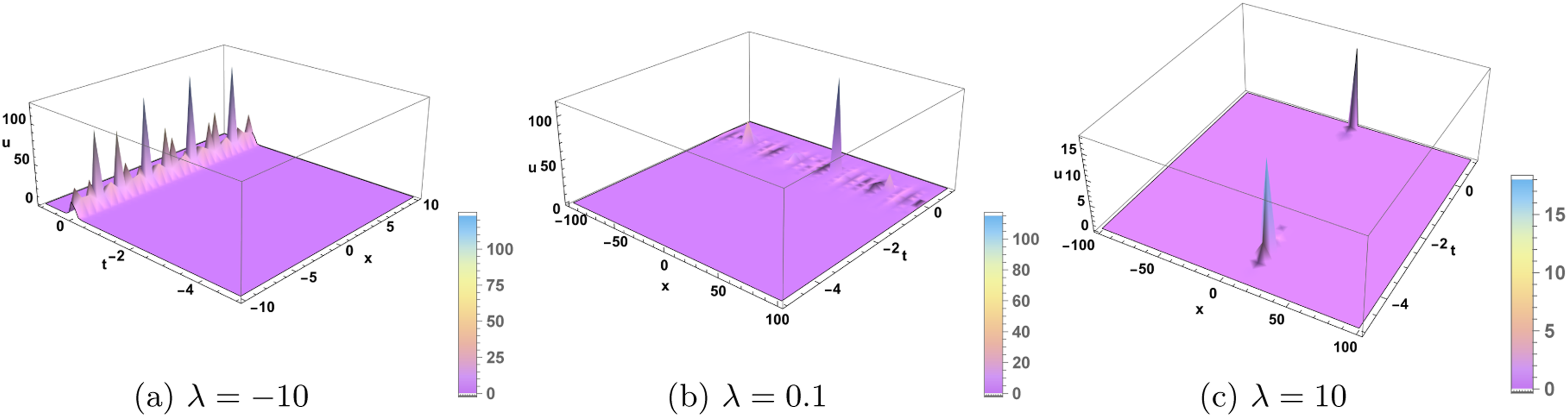

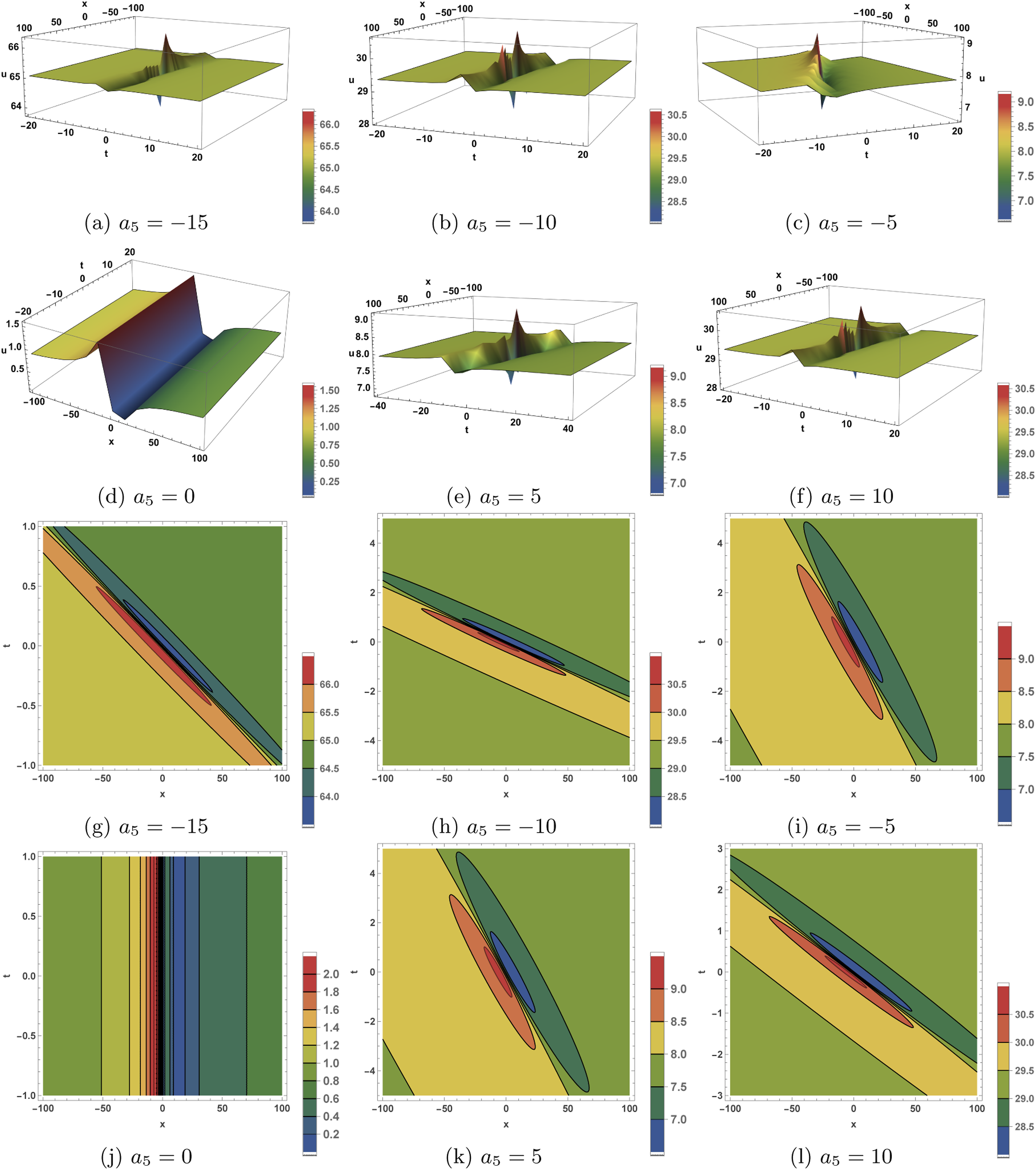
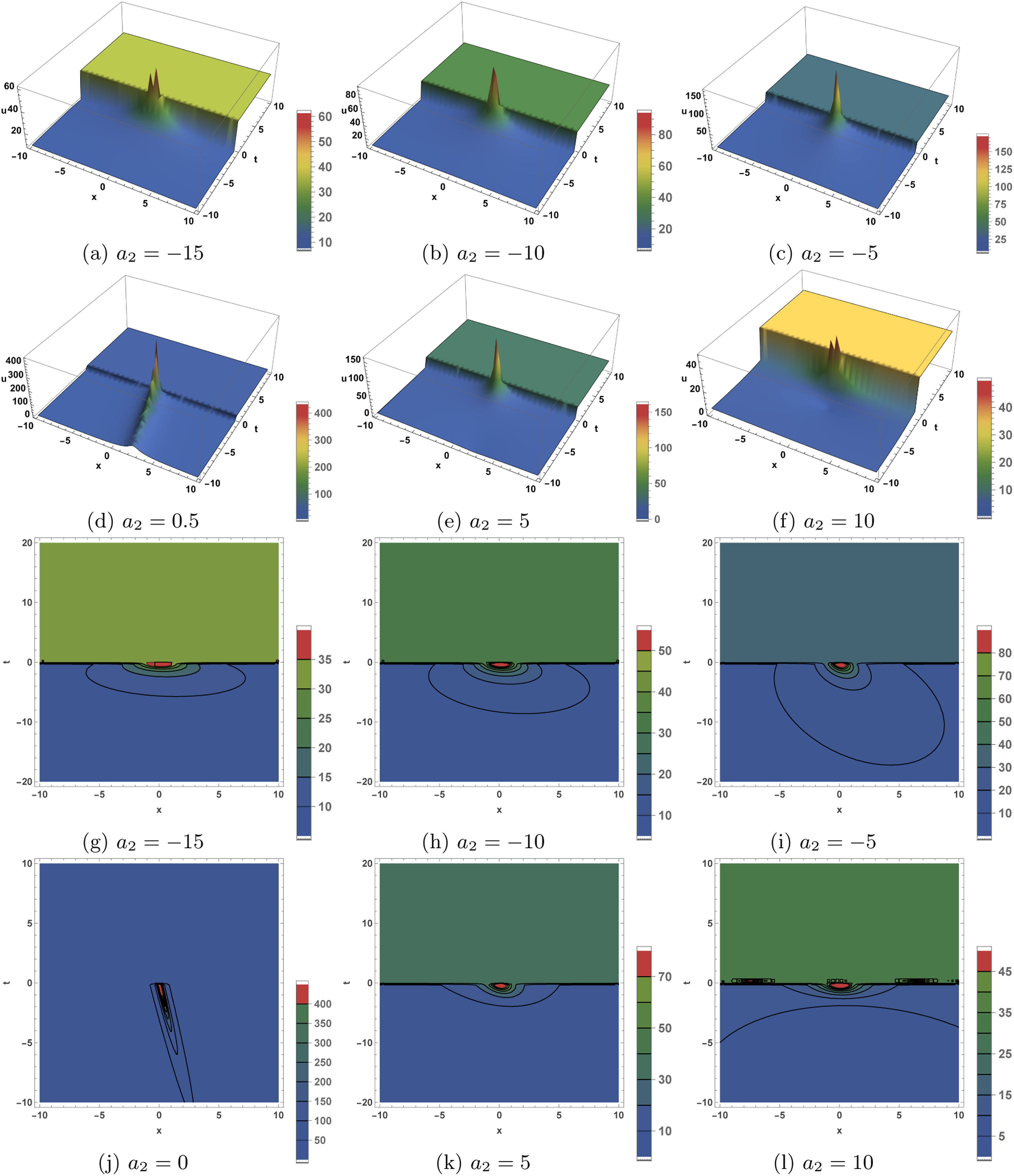
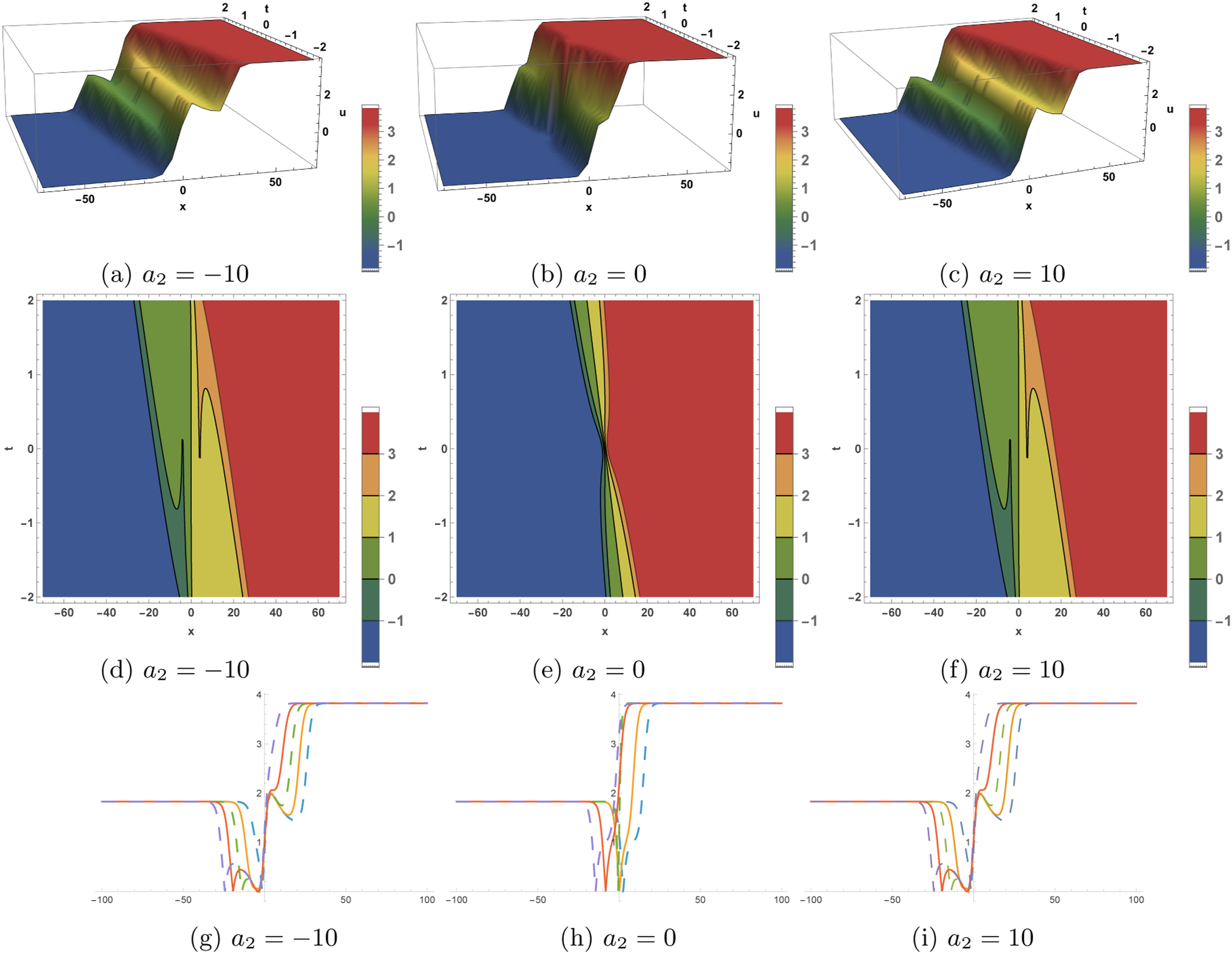
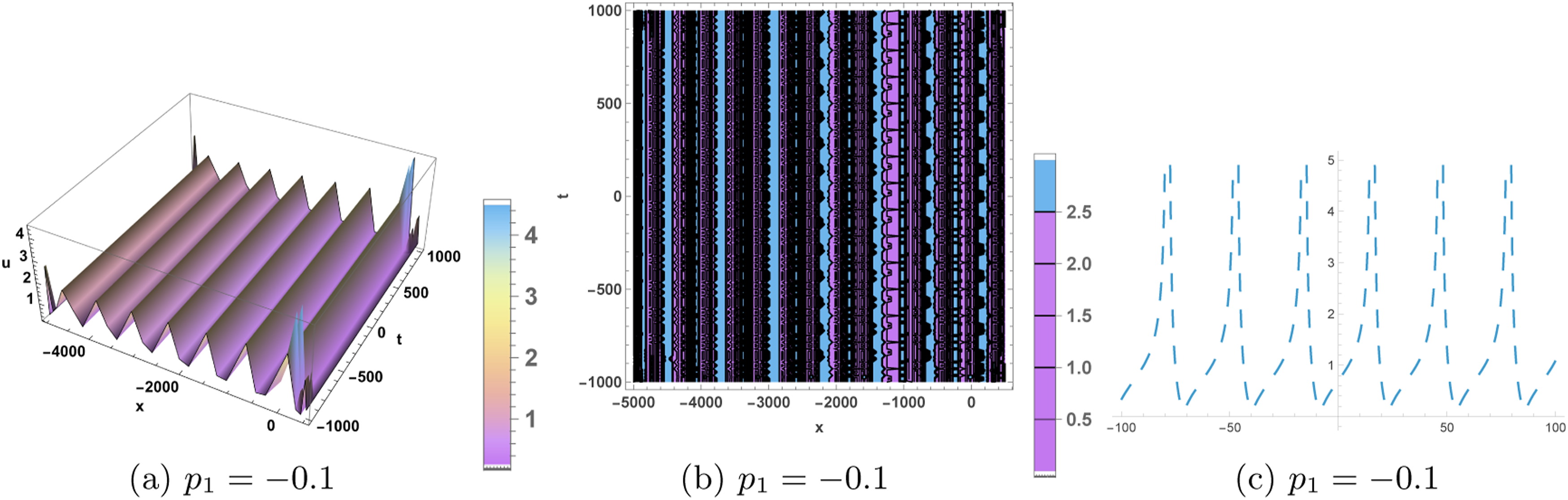
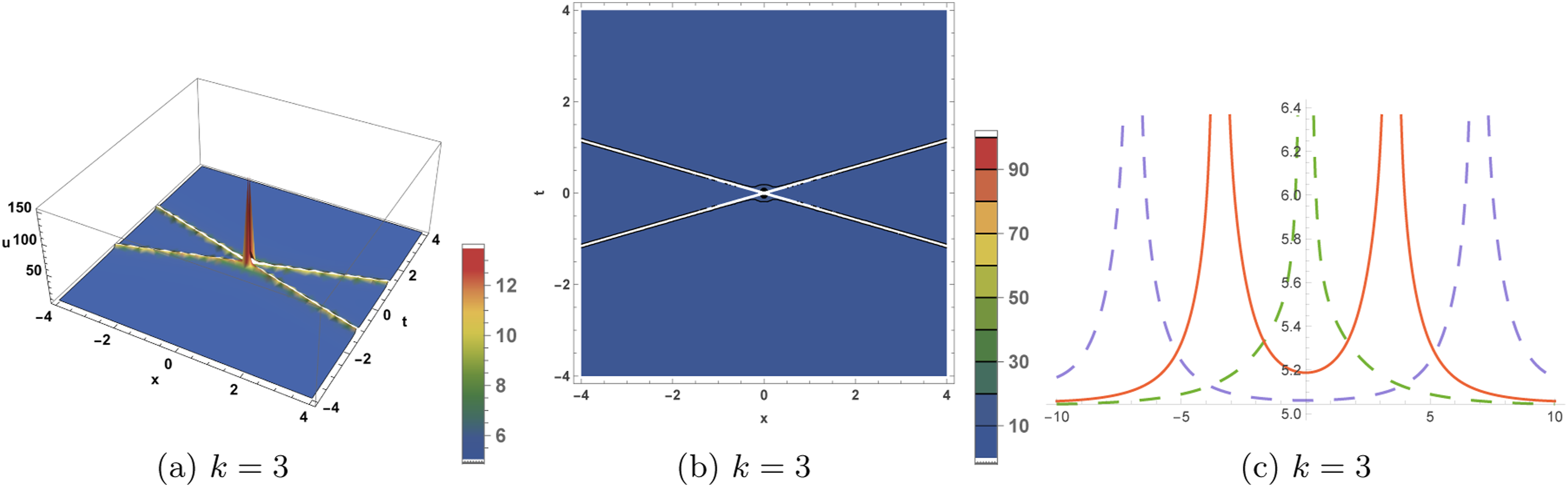
Figure 4 depicts the evolution for LP in Eq. (71) is made with p₁ = 4, a₄ = 3, m = 1, b₁ = 1, b = −2, a₅ = 2, showing the interaction between localized lump peaks and periodic wave backgrounds. The top panels (a–f) illustrate the 3D profiles, while the bottom panels (g–l) present the corresponding contour plots, highlighting the transition of periodic patterns and localization as a₂ varies. Figure 5 displays evolution of rogue waves in Eq. (74) for different a₂ values. (a–c) 3D profiles of u(x, t); (d–f) corresponding contour plots; (g–i) 2D views along x. a₂ = −10, 0, 10 Parameters: p₁ = 3, m = 1.5, b₁ = 1, b = 2, a₅ = 3. Figure 6 shows 3D, contour and 2D profiles of the manifold periodic solution u₅(x, t) for the parameter values a₁ = 1, a₂ = 0.5, a₃ = 0, d₁ = 0.8, d₂ = 1, a₆ = 1, h₂ = 0.5, and m = 1. (a) 3D shape at a₁ = −30, (b) contour profile at a₁ = −30, and (c) 2D profile at a₁ = −30 respectively. Figure 7 represents 3D, contour and 2D shapes MB in Eq. (80) are formed with the value of b = 3. (a) 3D shape at p₁ = −0.1, (b) contour profile at p₁ = −0.1, and (c) 2D profile at p₁ = −0.1 respectively. Figure 8 shows graphs for KMB (Eq. (83)) with b = 4, a₁ = −5. (a) 3D shape at p₁ = −0.1, (b) contour profile at p₁ = −0.1, and (c) 2D profile at p₁ = −0.1. Figure 9 interprets Graphs for GB in Eq. (88) with k = 10, b = 2, m = 1, σ = 0.5. (a) 3D shape, (b) contour profile, and (c) 2D profile respectively. Figure 10 displays 3D, contour and 2D shapes of AB in Eq. (91) are formed with the values of ω = 1, k = 3, m = 5, n = 10, p₀ = 4. (a) 3D shape at k = 3, (b) contour profile at k = 3, and (c) 2D profile at k = 3 respectively.

Figure 4.

The evolution for LP in Eq. (71) is made with p₁ = 4, a₄ = 3, m = 1, b₁ = 1, b = −2, a₅ = 2, showing the interaction between localized lump peaks and periodic wave backgrounds. The top panels (a–f) illustrate the 3D profiles, while the bottom panels (g–l) present the corresponding contour plots, highlighting the transition of periodic patterns and localization as a₂ varies.

Figure 5.

Evolution of rogue waves in Eq. (74) for different a₂ values. (a–c) 3D profiles of u(x, t); (d–f) corresponding contour plots; (g–i) 2D views along x. a₂ = −10, 0, 10 Parameters: p₁ = 3, m = 1.5, b₁ = 1, b = 2, a₅ = 3.

Figure 6.

3D, contour and 2D profiles of the manifold periodic solution u₅(x, t) for the parameter values a₁ = 1, a₂ = 0.5, a₃ = 0, d₁ = 0.8, d₂ = 1, a₆ = 1, h₂ = 0.5, and m = 1. (a) 3D shape at a₁ = −30, (b) contour profile at a₁ = −30, and (c) 2D profile at a₁ = −30 respectively.

Figure 7.

3D, contour and 2D shapes MB in Eq. (80) are formed with the value of b = 3. (a) 3D shape at p₁ = −0.1, (b) contour profile at p₁ = −0.1, and (c) 2D profile at p₁ = −0.1 respectively.

Figure 8.

Graphs for KMB (Eq. (83)) with b = 4, a₁ = −5. (a) 3D shape at p₁ = −0.1, (b) contour profile at p₁ = −0.1, and (c) 2D profile at p₁ = −0.1 respectively.

Figure 9.

Graphs for GB in Eq. (88) with k = 10, b = 2, m = 1, σ = 0.5. (a) 3D shape, (b) contour profile, and (c) 2D profile respectively.

Figure 10.

3D, contour and 2D shapes of AB and x-type wave in Eq. (91) are formed with the values of ω = 1, k = 3, m = 5, n = 10, p₀ = 4. (a) 3D shape at k = 3, (b) contour profile at k = 3, and (c) 2D profile at k = 3 respectively.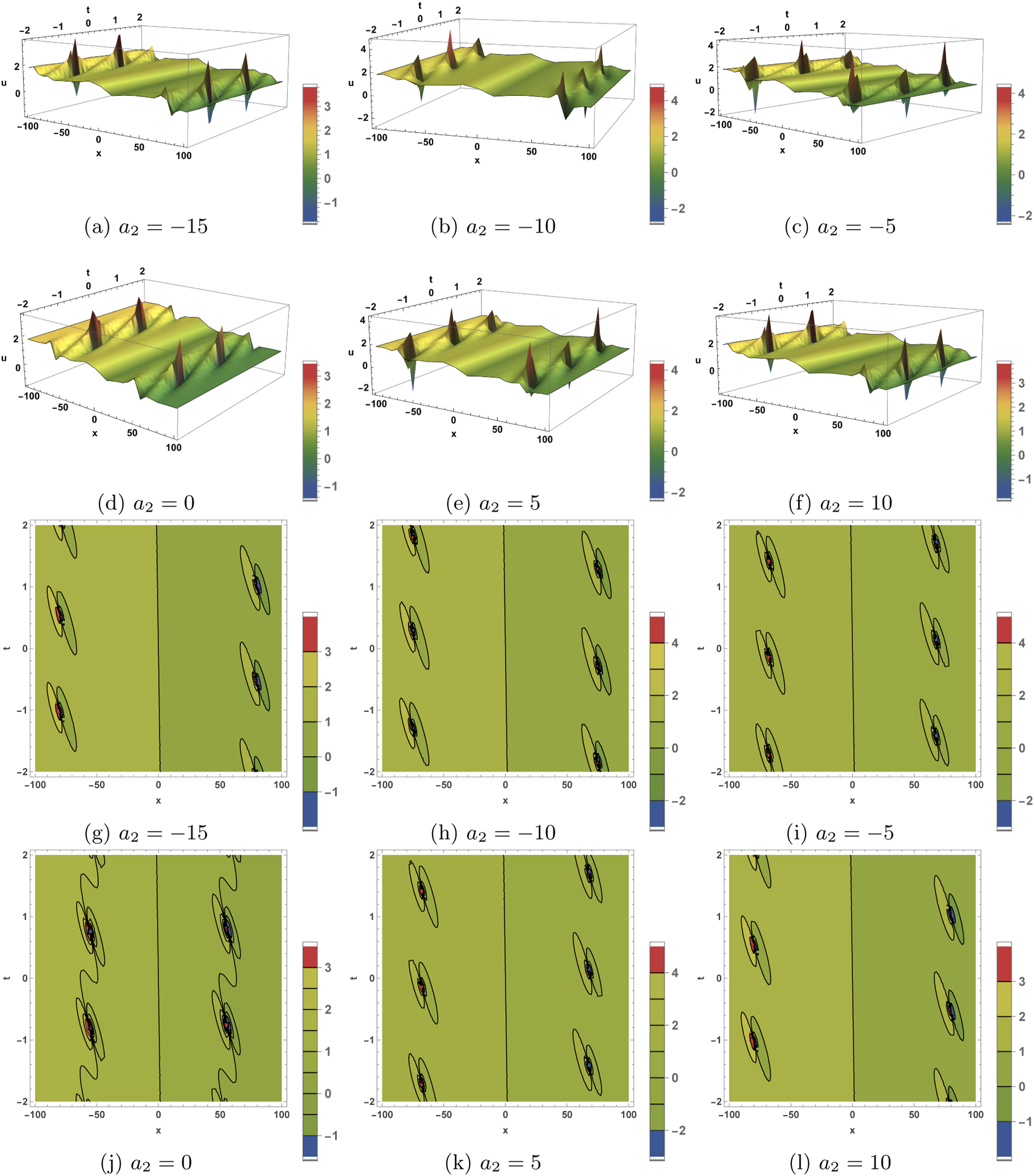

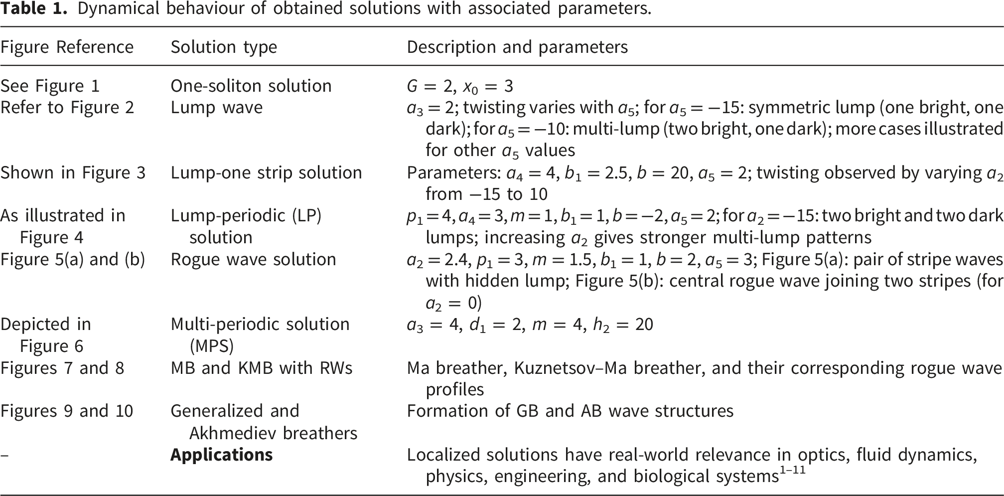
Since our work focuses on analytical solutions obtained via the Lax pair and Darboux transformation, the concept of “accuracy” here refers to the exactness and internal consistency of the solutions rather than approximation errors. All solutions presented are exact within the framework of the gFW equation. For practical applications, the accuracy of the model in representing real-world systems depends on how well the gFW equation itself approximates the physical system under consideration (e.g., shallow water waves, optical pulses, or plasma waves). In this context, the derived analytical solutions provide benchmark results that can be used to validate numerical simulations or experimental observations. To clarify this, our manuscript emphasizing that: The analytical solutions are exact solutions of the generalized FW equation. Their predictive value for physical systems depends on the applicability of the gFW model to the specific context. These solutions serve as references for evaluating numerical methods and understanding qualitative behaviors of nonlinear waves. For the geometry of our obtained solutions, see Table 1:

Table 1.

Dynamical behaviour of obtained solutions with associated parameters.

Figure Reference	Solution type	Description and parameters
See Figure 1	One-soliton solution	G = 2, x₀ = 3
Refer to Figure 2	Lump wave	a₃ = 2; twisting varies with a₅; for a₅ = −15: symmetric lump (one bright, one dark); for a₅ = −10: multi-lump (two bright, one dark); more cases illustrated for other a₅ values
Shown in Figure 3	Lump-one strip solution	Parameters: a₄ = 4, b₁ = 2.5, b = 20, a₅ = 2; twisting observed by varying a₂ from −15 to 10
As illustrated in Figure 4	Lump-periodic (LP) solution	p₁ = 4, a₄ = 3, m = 1, b₁ = 1, b = −2, a₅ = 2; for a₂ = −15: two bright and two dark lumps; increasing a₂ gives stronger multi-lump patterns
Figure 5(a) and (b)	Rogue wave solution	a₂ = 2.4, p₁ = 3, m = 1.5, b₁ = 1, b = 2, a₅ = 3; Figure 5(a): pair of stripe waves with hidden lump; Figure 5(b): central rogue wave joining two stripes (for a₂ = 0)
Depicted in Figure 6	Multi-periodic solution (MPS)	a₃ = 4, d₁ = 2, m = 4, h₂ = 20
Figures 7 and 8	MB and KMB with RWs	Ma breather, Kuznetsov–Ma breather, and their corresponding rogue wave profiles
Figures 9 and 10	Generalized and Akhmediev breathers	Formation of GB and AB wave structures
–	Applications	Localized solutions have real-world relevance in optics, fluid dynamics, physics, engineering, and biological systems^1–11

15. Concluding remarks

In this paper, we have derived a wide class of exact solutions to the generalized Fornberg–Whitham equation using the Lax pair structure, Darboux transformation, and appropriate variable transformations. The obtained solutions include one-soliton waves, breather solutions, lump structures, lump–1-strip, lump–periodic, manifold periodic, and rogue wave solutions. In particular, the existence of multiple-lump wave configurations under suitable parameter choices highlights the rich nonlinear dynamics supported by the model. Moreover, we have constructed Ma breathers, Kuznetsov–Ma breathers along with their corresponding rogue waves, as well as generalized and Akhmediev breathers. The influence of various parameters on the structure and evolution of these solutions has been illustrated through numerical visualizations, providing insight into their physical characteristics and interactions.

Despite these significant contributions, certain limitations remain in the present study. The analysis is primarily restricted to exact analytical solutions of an idealized and integrable (or near-integrable) form of the system, without considering dissipative effects, variable topography, or external forcing terms that are often present in real physical environments. Furthermore, the stability and robustness of the obtained solutions under perturbations have not been rigorously analyzed, and experimental validation or direct comparison with observational data is beyond the scope of this work.

Future research can address these limitations by extending the present framework to non-integrable, fraction gFW-equation and perturbed systems, incorporating physical effects such as viscosity, variable bathymetry, and stochastic forcing. In addition, stability analysis using spectral methods or numerical simulations would provide deeper insight into the persistence of these wave structures in realistic conditions. The development of data-driven approaches, such as machine learning techniques, may further enhance the prediction and control of extreme wave events. Finally, applying the obtained solutions to real world scenarios such as oceanic rogue waves, optical pulse propagation, and plasma wave dynamics would help bridge the gap between theoretical modeling and practical applications.

Footnotes

Ethical considerations

I declare that this manuscript represents my independent work and has been revised in accordance with the reviewers’ suggestions. Except for appropriately cited references, it contains no previously published material or contributions from other individuals or research groups.

Author contributions

Sarfaraz Ahmed: Writing original draft, Visualization, Investigation, Aly R. Seadawy: Software, Methodology, Validation, Syed Rizvi: Resources, Project administration, Writing review & editing, Ibtehal Alazman: Conceptualization, Data curation.

Funding

The authors disclosed receipt of the following financial support for the research, authorship, and/or publication of this article: This work was supported and funded by the Deanship of Scientific Research at Imam Mohammad Ibn Saud Islamic University (IMSIU) (grant number IMSIU-DDRSP2602).

Declaration of conflicting interests

The authors declared no potential conflicts of interest with respect to the research, authorship, and/or publication of this article.

References

Syed

Aldawish

Rizvi

STR

, et al. Bilinear neural network solutions for nonlinear waves in the Sawada–Kotera model studied in heat transfer. Eur. Phys. J. Plus 2025; 140: 835.

Ahmed

Aldawish

Rizvi

STR

, et al. Iterative Investigation of the Nonlinear Fractional Cahn–Allen and Fractional Clannish Random Walker’s Parabolic Equations by Using the Hybrid Decomposition Method. Fractal Fract 2025; 9: 656. https://doi.org/10.3390/fractalfract9100656

Seadawy

Ali

Radwan

, et al. Solitary wave solutions for the conformable time-fractional coupled Konno-Oono model via applications of three mathematical methods. AIMS Mathematics 2025; 10(7): 16027–16044. https://doi.org/10.3934/math.2025718

Mehanna

Alazman

Seadawy

. Comprehensive study of a (3+1)-dimensional nonlinear Vakhnenko-Parkes dynamical equation with applications in nonlinear wave propagation in relaxing media. AIMS Mathematics 2025; 10(11): 25206–25226. https://doi.org/10.3934/math.20251116

Seadawy

Rizvi

STR

Ahmad

, et al. lump-one stripe, multiwave and breather solutions for the Hunter–Saxton equation. Open Physics 2021; 19(1): 1–10. https://doi.org/10.1515/phys-2020-0224

Bilal

Seadawy

Younis

, et al. Analytical wave structures in plasma physics modelled by Gilson-Pickering equation by two integration norms. Results in Physics 2021: 23–103959.

Ali

Alazman

Rizvi

STR

, et al. Mathematical modeling and symmetry analysis of the impact of vaccination on the dynamics of influenza virus disease. Eur. Phys. J. Plus 2025; 140: 1150.

Rizvi

STR

Aldawish

Ahmed

, et al. Abundant analytical solutions for width-Burger equation: M-shaped, multiwave, breathers and their interactions. Boundary Value Problems, 2025) 2025, p. 178.

Rizvi

STR

Alazman

Seadawy

, et al. Elliptic Functions and Advanced Analysis of Soliton Solutions for the Dullin–Gottwald–Holm Dynamical Equation with Applications of Mathematical Methods. Symmetry 2025; 17: 1773. https://doi.org/10.3390/sym17101773

10.

Tariq

Zainab

Seadawy

, et al. On some novel optical wave solutions to the paraxial M-fractional nonlinear Schrödinger dynamical equation. Optical and Quantum Electronics 2021; 53(5): 1–14. https://doi.org/10.1007/s11082-021-02855-6

11.

Shahroz Khalid

Alazman

Rizvi

STR

, et al. Conformable Gross–Pitaevskii dynamical equation: Soliton solutions, energy balance, and nonlinear dynamics. Modern Physics Letters AVol 2025; 40(35): 2550173. https://doi.org/10.1142/s0217732325501731

12.

Bilal

Seadawy

Younis

, et al. Dispersive of propagation wave solutions to unidirectional shallow water wave Dullin–Gottwald–Holm system and modulation instability analysis. Mathematical Methods in the Applied Sciences 2021; 44(5): 4094–4104. https://doi.org/10.1002/mma.7013

13.

Iqbal

Seadawy

, Dispersive solitary wave solutions of nonlinear further modified Kortewege-de Vries dynamical equation in a unmagnetized dusty plasma via mathematical methods, Modern Physics Letters A 2018; 33(2018): 1–19. 1850217. https://doi.org/10.1142/s0217732318502176

14.

Younis

Younas

Bilal

, et al. Investigation of optical solitons with Chen–Lee–Liu equation of monomode fibers by five free parameters. Indian Journal of Physics 2021; 96: 1–8. https://doi.org/10.1007/s12648-021-02077-2

15.

Seadawy

Iqbal

. Construction of new solitary wave solutions of generalized Zakharov-Kuznetsov-Benjamin-Bona-Mahony and simplified modified form of Camassa-Holm equations. Open Physics 2018; 16: 896–909. https://doi.org/10.1515/phys-2018-0111

16.

Liu

Wazwaz

. Novel high-order breathers and rogue waves in the Boussinesq equation via determinants. International Journal of Modern Physics B 2020; 43(6): 3701–3715. https://doi.org/10.1002/mma.6148

17.

Osman

. Multi-soliton rational solutions for some nonlinear evolution equations. Applied Mathematics Letters 2014; 12(3): 126–136. https://doi.org/10.1515/phys-2015-0056

18.

Gao

Guo

Shan

, et al. Magneto-optical/ferromagnetic-material computation: Bäcklund transformations, bilinear forms and N solitons for a generalized (3 + 1)-dimensional variable-coefficient modified Kadomtsev–Petviashvili system. Applied Mathematics Letters 2021; 111: 106627.

19.

Kaur

Wazwaz

. Einstein’s vacuum field equation: Painlevé analysis and Lie symmetries. Waves in Random and Complex Media 2021; 31(2): 199–206. https://doi.org/10.1080/17455030.2019.1574410

20.

Nielsen

Garbin

, et al. Spontaneous symmetry breaking of dissipative optical solitons in a two-component Kerr resonator. Nature Communications 2021; 12(1): 1–9. https://doi.org/10.1038/s41467-021-24251-0

21.

Seadawy

Bilal

Younis

, et al. Analytical mathematical approaches for the double-chain model of DNA by a novel computational technique. Chaos, Solitons and Fractals 2021; 144: 110669.

22.

Zayed

Alngar

Biswas

, et al. Solitons and conservation laws in magneto–optic waveguides with generalized Kudryashov’s equation. Chinese Journal of Physics 2021; 69: 186–205. https://doi.org/10.1016/j.cjph.2020.11.026

23.

Arnous

Biswas

Ekici

, et al. Optical solitons and conservation laws of Kudryashov’s equation with improved modified extended tanh-function. Optik 2021; 225: 165406.

24.

Wazwaz

. The Hirota bilinear method and the tanh–coth method for multiple-soliton solutions of the Sawada–Kotera–Kadomtsev–Petviashvili equation. Applied Mathematics and Computation 2008; 200: 160–166. https://doi.org/10.1016/j.amc.2007.11.001

25.

Seadawy

Ahmed

Rabie

, et al. Chirp-free optical solitons in fiber Bragg gratings with dispersive reflectivity having polynomial law of nonlinearity. Optik 2021; 225: 165681. https://doi.org/10.1016/j.ijleo.2020.165681

26.

Seadawy

Cheemaa

. Applications of extended modified auxiliary equation mapping method for high-order dispersive extended nonlinear Schrödinger equation in nonlinear optics. Modern Physics Letters B 2019; 33(18): 1950203. https://doi.org/10.1142/s0217984919502038

27.

Kumar

. Lie symmetry analysis for obtaining the abundant exact solutions, optimal system and dynamics of solitons for a higher-dimensional Fokas equation. Chaos, Solitons and Fractals 2021; 142: 110507.

28.

Noeiaghdam

Sidorov

Wazwaz

, et al. The Numerical Validation of the Adomian Decomposition Method for Solving Volterra Integral Equation with Discontinuous Kernels Using the CESTAC Method. Mathematics 2021; 9(3): 260. https://doi.org/10.3390/math9030260

29.

Dai

. symmetry breaking bifurcation and stability of two-dimensional optical solitons supported by fractional diffraction. Optics Express 2021; 29(3): 3193–3210. https://doi.org/10.1364/oe.415028

30.

Gaber

Aljohani

Ebaid

, et al. The generalized Kudryashov method for nonlinear space–time fractional partial differential equations of Burgers type. Nonlinear Dyn 2019; 95(1): 361–368. https://doi.org/10.1007/s11071-018-4568-4

31.

Rizvi

STR

Ali

Ahmad

. Optical solitons for Biswas–Milovic equation by new extended auxiliary equation method. Optik 2020; 204: 164181.

32.

Farah

Seadawy

Ahmad

, et al. Interaction properties of soliton molecules and Painleve analysis for nano bioelectronics transmission model. Optical and Quantum Electronics 2020; 52(7): 1–15. https://doi.org/10.1007/s11082-020-02443-0

33.

. Variational principle and periodic solution of the Kundu-Mukherjee-Naskar equation. Results in Physics 2020: 17–103031.

34.

Ghaffar

Ali

Ahmed

, et al. A novel analytical technique to obtain the solitary solutions for nonlinear evolution equation of fractional order. Advances in Difference Equations 2020; 1: 1–15. https://doi.org/10.1186/s13662-020-02751-5

35.

Mohammadian

. A fast insight into high-accuracy nonlinear frequency estimation of stringer-stiffened shells. Facta Universitatis, Series: Mechanical Engineering 2025; 23(4): 787–806. https://doi.org/10.22190/fume250525028h

36.

, et al. A modified frequency formulation for nonlinear mechanical vibrations. Facta Universitatis, Series: Mechanical Engineering 2025; 23(2): 197–210. https://doi.org/10.22190/fume250526022h

37.

. Frequency-amplitude relationship in nonlinear oscillators with irrational nonlinearities. Spectrum of Mechanical Engineering and Operational Research 2025; 2(1): 121–129. https://doi.org/10.31181/smeor21202535

38.

Milic

Marinkovic

Cojbasic

. Geometrically nonlinear analysis of piezoelectric active laminated shells by means of isogeometric FE formulation. Facta Universitatis, Series: Mechanical Engineering 2025; 32(2): 387–405. https://doi.org/10.22190/fume050123059m

39.

Friedlander

Vishik

. Lax pair formulation for the Euler equation. Physics Letters A 1990; 148(6): 313–319. https://doi.org/10.1016/0375-9601(90)90809-3

40.

Mabrouk

Rashed

. Analysis of (3+ 1)-dimensional Boiti–Leon–Manna–Pempinelli equation via Lax pair investigation and group transformation method. Computers and Mathematics with Applications 2017; 74(10): 2546–2556. https://doi.org/10.1016/j.camwa.2017.07.033

41.

Yuan

Tian

, et al. Lax pair, binary Darboux transformation and dark solitons for the three-component Gross–Pitaevskii system in the spinor Bose–Einstein condensate. Nonlinear Dynamics 2020; 99(4): 3001–3011. https://doi.org/10.1007/s11071-020-05483-z

42.

. Lax pair, Darboux transformation and Nth-order rogue wave solutions for a (2+ 1)-dimensional Heisenberg ferromagnetic spin chain equation. Computers and Mathematics with Applications 2019; 77(2): 514–524. https://doi.org/10.1016/j.camwa.2018.09.054

43.

Ding

Gao

Deng

, et al. Lax pair, conservation laws, Darboux transformation, breathers and rogue waves for the coupled nonautonomous nonlinear Schrödinger system in an inhomogeneous plasma. Chaos, Solitons and Fractals 2020; 133: 109580.

44.

Yang

Tian

, et al. Lax pair, conservation laws, Darboux transformation and localized waves of a variable-coefficient coupled Hirota system in an inhomogeneous optical fiber. Chaos, Solitons and Fractals 2021; 150: 110487. https://doi.org/10.1016/j.chaos.2020.110487

45.

Tian

Chai

, et al. Lax pair, Darboux transformation, vector rational and semi-rational rogue waves for the three-component coupled Hirota equations in an optical fiber. The European Physical Journal Plus 2019; 134(5): 213. https://doi.org/10.1140/epjp/i2019-12515-4

46.

Camacho

Rosa

Gandarias

, et al. Classical symmetries, travelling wave solutions and conservation laws of a generalized Fornberg–Whitham equation. Journal of Computational and Applied Mathematics 2017; 318: 149–155. https://doi.org/10.1016/j.cam.2016.11.017

47.

Itasaka

. Wave-breaking phenomena and global existence for the generalized Fornberg-Whitham equation. Journal of Mathematical Analysis and Applications 2021; 502(1): 125247. https://doi.org/10.1016/j.jmaa.2021.125247

48.

Jang

Okawachi

, et al. Breather soliton dynamics in microresonators. Nature communications 2017; 8(1): 1–7. https://doi.org/10.1038/ncomms14569

49.

Chen

. Interaction solutions to nonlinear partial differential equations via Hirota bilinear forms: One-lump-multi-stripe and one-lump-multi-soliton types. Nonlinear Dynamics 2021; 103(1): 947–977. https://doi.org/10.1007/s11071-020-06068-6

50.

Saut

Sun

Wang

, et al. Wave Breaking for the Generalized Fornberg-Whitham Equation. SIAM Journal on Mathematical Analysis 2024; 56(4): 4440–4465. https://doi.org/10.1137/23m1603431

51.

Nazari-Golshan

. Exploring new traveling wave solutions by solving the nonlinear space–time fractal Fornberg-Whitham equation. Scientific Reports 2024; 14(1): 18642. https://doi.org/10.1038/s41598-024-66298-1

52.

Noor

Hammad

MMA

Shah

, et al. Numerical investigation of fractional-order fornberg–whitham equations in the framework of aboodh transformation. Symmetry 2023; 15(7): 1353. https://doi.org/10.3390/sym15071353

53.

Sartanpara

Meher

. The generalized time fractional Fornberg-Whitham equation: An analytic approach. Partial Differential Equations in Applied Mathematics 2022; 5(1): 100350. https://doi.org/10.1016/j.padiff.2022.100350

54.

Geng

Shen

Xue

. A new nonlinear wave equation: Darboux transformation and soliton solutions. Wave Motion 2018; 79: 44–56. https://doi.org/10.1016/j.wavemoti.2018.02.009

55.

Olver

. Darboux’theorem for Hamiltonian differential operators. Journal of differential equations 1988; 71(1): 10–33. https://doi.org/10.1016/0022-0396(88)90036-8

56.

Oevel

. Darboux theorems and Wronskian formulas for integrable systems. Physica A: Statistical Mechanics and its Applications 1993; 195(3): 533–576. https://doi.org/10.1016/0378-4371(93)90174-3

57.

Wang

. Lump and interaction solutions to the (2 + 1)-dimensional Burgers equation. Applied Mathematics Letters 2018; 85: 27–34. https://doi.org/10.1016/j.aml.2018.05.010

58.

Zhou

Manukure

. Lump and lump-soliton solutions to the Hirota Satsuma equation. InCommunications in Nonlinear Science and Numerical Simulation 2019; 68: 56–62. https://doi.org/10.1016/j.cnsns.2018.07.038

59.

Wang

. Lump and interaction solutions to the (2+ 1)-dimensional Burgers equation. Applied Mathematics Letters 2018; 85: 27–34. https://doi.org/10.1016/j.aml.2018.05.010

60.

Khan

Lump

. multi-lump, cross kinky-lump and manifold periodic-soliton solutions for the (2+ 1)-D Calogero–Bogoyavlenskii–Schiff equation. Heliyon 2020; 6(4): 03701.

61.

. N-solitons, breathers and rogue waves for a generalized Boussinesq equation. International Journal of Computer Mathematics 2020; 97(8): 1648–1661. https://doi.org/10.1080/00207160.2019.1639678

62.

Singh

Sakkaravarthi

Murugesan

, et al. Benjamin-Ono equation: Rogue waves, generalized breathers, soliton bending, fission, and fusion. The European Physical Journal Plus 2020; 135(10): 1–17. https://doi.org/10.1140/epjp/s13360-020-00808-8

63.

Dudley

Genty

Dias

, et al. Modulation instability, Akhmediev Breathers and continuous wave supercontinuum generation. Optics express 2009; 17(24): 21497–21508. https://doi.org/10.1364/OE.17.021497

64.

Abidi

Omrani

. The homotopy analysis method for solving the Fornberg–Whitham equation and comparison with Adomian’s decomposition method. Computers and Mathematics with Applications 2010; 59(8): 2743–2750. https://doi.org/10.1016/j.camwa.2010.01.042

65.

Manafian

Lakestani

. The classification of the single traveling wave solutions to the modified Fornberg–Whitham equation. International Journal of Applied and Computational Mathematics 2017; 3(4): 3241–3252. https://doi.org/10.1007/s40819-016-0288-y

66.

Wei

. Wave breaking analysis for the Fornberg–Whitham equation. Journal of Differential Equations 2018; 265(7): 2886–2896. https://doi.org/10.1016/j.jde.2018.04.054

67.

Hormann

. Solution concepts, well-posedness, and wave breaking for the Fornberg–Whitham equation. Monatshefte fur Mathematik 2018; 195(3): 421–449. https://doi.org/10.1007/s00605-020-01504-6

68.

Ahmad

Seadawy

Ganie

, et al. Approximate Numerical solutions for the nonlinear dispersive shallow water waves as the Fornberg–Whitham model equations. Results in Physics 2021; 22(7): 103907. https://doi.org/10.1016/j.rinp.2021.103907

69.

Lai

. The entropy weak solution to a generalized Fornberg–Whitham equation. Boundary Value Problems 2020; 1: 791–810.

70.

Dai

Yuan

. The classification and representation of single traveling wave solutions to the generalized Fornberg–Whitham equation. Applied Mathematics and Computation 2014; 242: 729–735. https://doi.org/10.1016/j.amc.2014.06.049

71.

Zhang

Muhammad

, et al. Lump, periodic lump and interaction lump stripe solutions to the (2 + 1)-dimensional B-type Kadomtsev–Petviashvili equation. Modern Physics Letters B 2018; 32(07): 1850106. https://doi.org/10.1142/s0217984918501063

72.

. multiple-lump waves for a (3 + 1)-dimensional Boiti–Leon–Manna–Pempinelli equation arising from incompressible fluid. Computers and Mathematics with Applications 2018; 76(1): 204–214. https://doi.org/10.1016/j.camwa.2018.04.015

73.

Ahmed

Seadawy

. Kinky breathers, W-shaped and multi-peak solitons interaction in (2 + 1)-dimensional nonlinear Schrödinger equation with Kerr law of nonlinearity. The European Physical Journal Plus 2019; 134(3): 1–10. https://doi.org/10.1140/epjp/i2019-12482-8

74.

Ahmed

Seadawy

. M-shaped rational solitons and their interaction with kink waves in the Fokas–Lenells equation. Physica Scripta 2019; 94: 055205. https://doi.org/10.1088/1402-4896/ab0455

75.

Manafian

Lakestani

. New improvement of the expansion methods for solving the generalized Fitzhugh–Nagumo equation with time-dependent coefficients. Int. J. Eng. Math 2015; 2015: 107978–108035. https://doi.org/10.1155/2015/107978