A flexible observed factor model with separate dynamics for the factor volatilities and their correlation matrix

Abstract

In this article, we consider a novel regression model with observed factors. To allow for the prediction of future observations, we model the observed factors using a flexible multivariate stochastic volatility (MSV) structure with separate dynamics for the volatilities and the correlation matrix. The correlation matrix of the factors is time varying, and its evolution is described by an inverse Wishart process. We develop an estimation procedure based on Bayesian Markov chain Monte Carlo methods, which has two major advantages compared to existing methods for similar models in the literature. First, the procedure is computationally more efficient. Second, it can be applied to calculate the predictive distributions for future observations. We compare the proposed model with other multivariate volatility models using Fama-French factors and portfolio weighted return data. The result shows that our model has better predictive performance.

Keywords

1 Introduction

Over the last two decades, multivariate stochastic volatility (MSV) models have become an important class in financial econometrics, largely due to the successful utilization of Bayesian Markov chain Monte Carlo (MCMC) methods in model estimation. Recent developments in the MSV literature focus on dimension reduction via factor analysis, given that the complexity of computation and the difficulty in model interpretation drastically increase as the dimension of data increases. Harvey et al. (1994) first discussed the MSV factor structure. Bayesian methodology was introduced to the factor MSV (FMSV) models by Jacquier et al. (1995), where the stochastic volatility (SV) process is imposed on the factor structure. Pitt and Shephard (1999), Chib et al. (2006) and Lopes and Carvalho (2007) consider different specifications that allow more complicated factor dynamics.

A common feature of these FMSV models is the diagonality restriction imposed on the factor correlation/covariance matrix, implying that the factors are uncorrelated. This assumption could be unrealistic in real problems, especially when the factors are observable. To relax the diagonality assumption in a time-varying framework, Philipov and Glickman (2006b) introduced a dynamic FMSV model in which the inverse factor covariance matrices are driven by Wishart processes. The model is a straightforward application of factor analysis to the work of Philipov and Glickman (2006a). The inverse Wishart specification introduced by Philipov and Glickman (2006a, 2006b) is appealing because it can be estimated via MCMC methods. Asai and McAleer (2009) (hereafter AM) propose a dynamic correlation MSV model (DCMSV) based on MCMC techniques, where the return series are directly modelled with SV processes and the covariance evolution is characterized by the inverse Wishart distribution. Since Philipov and Glickman (2006a, 2006b) and AM’s models have similarity on the covariance specification, following AM, in this article we term this class of models the ‘Wishart Inverse Covariance’ (WIC). Philipov and Glickman (2006a, 2006b) and AM demonstrate the usefulness of the WIC models in portfolio analysis and risk management. Moreover, AM show with real data that their WIC model works well in capturing the evolution of the correlation matrix, while the dynamic conditional correlation (DCC) GARCH (Engle, 2002) models fail.

There are several major issues in existent WIC MSV/FMSV models. First, the time effect among different series is controlled by only one scalar persistence parameter, which is likely to be too restrictive in practice. To resolve this issue, we propose an observed dynamic-correlation FMSV model (DCFMSV). The basic model form of DCFMSV is similar to that of AM, but the structure is applied to a factor model. Compared with the FMSV of Philipov and Glickman (2006b) (hereafter PG), DCFMSV provides more flexibility because it allows for different time effects on the factors by introducing separate SV processes. Due to the factor structure, applications of DCFMSV to large datasets can be more advantageous than AM’s DC-MSV model. Another issue with the WIC models lies in the MCMC implementation. Philipov and Glickman (2006a) and AM propose different MCMC methods to conduct the posterior simulation. However, these methods may be either time consuming or potentially inaccurate. We propose a computationally more efficient algorithm that is free from the potential inaccuracy. Moreover, because the algorithm treats the estimation of the parameters and the latent variables simultaneously, it improves the disadvantage of AM’s two-stage method that cannot be easily utilized for future prediction.

This article makes a two-fold contribution. First, we introduce a novel flexible factor model to the WIC MSV literature, where the factors are observable. The model is an extension of AM’s DC-MSV to the factor model framework. Second, we develop a computationally more efficient MCMC algorithm that applies to the whole class of WIC models. The algorithm not only improves computational efficiency but also makes forecasting feasible and thus significantly increases the usefulness of the WIC models.

The remainder of the article is organized as follows. Section 2 presents the model and discusses the Bayesian estimation. Section 3 introduces the MCMC algorithm and conducts a Monte Carlo study using real data to compare the computational efficiency between the proposed scheme and AM’s method. Section 4 provides an empirical example using Fama-French’s factors and portfolio weighted return data. Based on the quality of one-step-ahead predictions, the DCFMSV is compared with AM’s DC-MSV, PG’s FMSV and the well-known DCC-GARCH model. Section 5 presents concluding remarks and some further discussions.

2 The model

2.1 Model specification

Suppose that at time t we have a p-dimensional vector of asset returns, y _t , and q underlying observed factors, f _t , such that y (2.1) _t B f _t e _t

where B is the loading matrix and { f _t , t ≥1} and { e _t , t ≥ 1} are independent stochastic processes. The e _t are also assumed to be independent with $e_{t} \sim N_{p} (e_{t} | 0, Ω), Ω = diag (σ_{1}^{2}, ..., σ_{p}^{2}),$ where N_p( X |  , ) is a p-dimensional multivariate normal density in X with mean  and covariance matrix ∑. The model for the factors is as follows:

f_{t} = V_{t}^{1 / 2} ϵ_{t},

(2.2a)

V_{t}^{1 / 2} = d i a g (e^{h_{t 1} / 2}, e^{h_{t 2} / 2}, \dots, e^{h_{t q} / 2}) ​, q \leq p,

(2.2b)

h (2.2c) _t ₊₁ μ ϕ h _t μ  _t

h_{1 i} \sim N (h_{1 i} | μ_{i}, \frac{σ_{η, i}^{2}}{1 - ϕ_{i}^{2}}), i = 1, 2, \dots, q,

(2.2d)

where N(x|μ, ²) is a univariate normal density in x with mean μ and variance ², and ο is the element-wise multiplication operator. The stochastic sequences {ε_t, t ≥ 1} and { η _t , t ≥ 1} are independent with η _t also an independent sequence and _t(2.3a) P _t _q_t0 ∑,t

η_{t} \sim N q_{} (η_{t} | 0, Σ_{η}), Σ_{η} = d i a g (σ_{η, 1}^{2}, \dots, σ_{η, q}^{2}) .

(2.3b)

The covariance matrix ∑ε,t is a correlation matrix which is obtained by standardizing the q × q stochastic covariance matrix P _t so that

Σ_{ϵ, t} = {(d i a g P_{t})}^{- \frac{1}{2}} P_{t} {(d i a g P_{t})}^{- \frac{1}{2}} .

(2.4)

The dynamics of P _t , and hence ∑_ε,t are given by the stationary autoregressive inverse Wishart process

P_{t + 1}^{- 1} | k, P_{t}^{- 1} \sim W_{q} (P_{t + 1}^{- 1} | k, S_{t}), S_{t} = \frac{1}{k} P_{t}^{- \frac{d}{2}} A P_{t}^{- \frac{d}{2}},

(2.5)

where Wq( X |k, S ) is a Wishart density in X with degrees of freedom (df) k ≥ q and the scale matrix S . The q × q matrix A is a symmetric positive definite matrix parameter, and d is a scalar parameter that accounts for the memory of the matrix process { P _t }. The matrix power operation $P_{t}^{- d / 2}$ is defined by a spectral decomposition. Similar to Philipov and Glickman (2006a), PG and AM, we set the initial value P ₀ to be P ₀ = I _q for convenience.

In the WIC context, there are two different ways to define the scale matrix. AM use Equation (2.5), while PG adopt a BEKK-type representation

S_{t} = \frac{1}{k} A^{\frac{1}{2}} {(P_{t}^{- 1})}^{d} (A^{\frac{1}{2}})',

(2.6)

where $A^{\frac{1}{2}}$ is defined by a Cholesky decomposition such that $A = A^{\frac{1}{2}} (A^{\frac{1}{2}})'$ . In either case, Philipov and Glickman (2006a) and AM show that log | P t| is a first-order autoregression with d being the autoregressive coefficient. If d ∈ (−1, 1), this first order autoregressive process is stationary.

Although the DCFMSV specification is similar to AM’s DC-MSV, the two models are fundamentally different in several aspects. First, AM adopt the settings (2.2a)–(2.5) to model the return series, while DCFMSV applies the settings to the observed factors. This difference is the main advantage of DCFMSV over DC-MSV, as the utilization of a factor structure largely reduces the computational cost and makes the results more interpretable. In the example given later, we have a dataset of 10 industry portfolios, which means for the modelling with DC-MSV, there are 55 elements to be estimated in the correlation matrix. However, if we apply DCFMSV with three common factors, the number of the correlation parameters is reduced to only six. As a consequence of the less complex dependence structure, the estimation result is much easier to interpret and the running time is drastically reduced. Another difference between DCFMSV and DC-MSV is in the sampling scheme. As will be discussed later, the algorithm we develop for DCFMSV can carry out broader analyses, such as forecasting.

2.2 Priors

There are two parameters in Equation (2.1), the measurement equation. For the idiosyncratic variances $Ω = diag (σ_{1}^{2}, \dots, σ_{p}^{2})$ , following Liesenfeld and Richard (2006), we assign independent inverse gamma priors $σ_{j}^{2} \sim I G (σ_{j}^{2} | s h a p e = ν_{0} / 2, s c a l e = ν_{0} s_{0} / 2)$ . In all our analyses, we use v₀ = 10 and s₀ = 0.01. This defines a vague prior which is commonly adopted in the literature. For the loading matrix B , following Jacquier et al. (1995), we choose the prior:

p (B | Ω) \propto | Ω |^{- p / 2} e t r (- \frac{1}{2} Ω^{- 1} B B') ​,

(2.7)

where etr( X ) means exp(trace( X )). This prior implies that the columns B _i of B are a priori independent, each with a prior N_p( B _i |0, Ω), which is uninformative relative to the data.

We adopt the priors suggested by Kim et al. (1998) for the SV parameters. For μ_i and $σ_{η, i}^{2}, i = 1, .., q,$ we assume that μ_i ∼ N (μ_i|0, 10) and $σ_{η, i}^{2} \sim I G (σ_{η, i}^{2} | 5, 0.05) .$ The prior for ϕ_i is a shifted and scaled beta distribution. Let $ϕ_{i} = 2 {\tilde{ϕ}}_{i} - 1$ where ${\tilde{ϕ}}_{i} \sim B e t a (ϕ^{(1)}, ϕ^{(2)}) .$ We choose ϕ⁽¹⁾ = 20 and ϕ⁽²⁾ = 1.5, implying a prior mean of 0.86.

Following PG and AM, the priors for the correlation-level parameters are chosen as follows: for A we specify the prior A ^–1 ∼ W_q( A ^–1|q, q^–1 I _q ). The degrees of freedom equals to q implies a very large spread, which defines an extremely diffuse prior. For d, we choose the vague prior d ∼ Unif(d|–1, 1). Finally, for k we set $k \sim λ_{0} e^{- λ_{0} k} I_{(q, \infty)} (k)$ . Note that the prior for k is a truncated exponential distribution with a rate parameter λ₀. Throughout the article we set λ₀ = 0.02. This implies a prior mean of 50 + q and a prior standard deviation of 50, indicating a very diffuse prior.

2.3 Bayesian estimation

2.3.1 Joint distribution

We estimate the model using an MCMC simulation method described in the following. Let the observed returns Y = { y _t } : T × p, the observed factors F = { f _t } : T × q, the log volatilities H = { h _t } : T × q, the normalized factors ε = { ε _t } : T × p, and the sequence of unnormalized covariance matrices P = { P _t , t = 1, …, T}. Let ω = { ω _i , i = 1, … q}, with ω _i = { μ _i , ϕ _i , σ _η,i , i = 1, …, q}, be the parameters of the volatilities of the factors.

The joint density of ( Y , F , H , ε , P , B , Ω, ω, A , d, k) is p(2.8) Y F H ε P B Ω ω Adk p(2.9) Y B F Ωp F H ε p H ω p ε P p P A dkp B ΩpΩp A pdpk

where

p (Y | B, F, Ω) = \prod_{t = 1}^{T} p (y_{t} | f_{t}, Ω),

(2.10a)

p (F | H, ϵ) = \prod_{t = 1}^{T} p (f_{t} | h_{t}, ϵ_{t}),

(2.10b)

p (h_{t} | ω) = p (h_{1} | ω) \prod_{t = 2}^{T} p (h_{t} | h_{t - 1}, ω),

p (h_{1} | ω) = \prod_{i = 1}^{q} p (h_{1 i} | ω_{i}), p (h_{t} | h_{t - 1}, ω) = \prod_{i = 1}^{q} p (h_{t i} | h_{t - 1, i}, ω_{i}),

(2.10c)

p (ϵ | P, A) = \prod_{t = 1}^{T} p (ϵ_{t} | P_{t}),

(2.10d)

p (P | A, d, k) = \prod_{t = 1}^{T} p (P_{t} | P_{t - 1}, A, d, k) .

(2.10e)

The densities p( y _t | f _t , Ω) in (2.10a) are given by Equation (2.1). The densities p( f _t | h _t , ε _t ) in (2.10b) are degenerate and are given by (2.2a). The densities p(h_1i| ω _i ) in (2.10c) are given by (2.2d), and the densities p( h _ti | h _t _–1,i, ω _i ) in (2.10c) are given by (2.2c). The densities p(  _t | P _t ) in (2.10d) are given by (2.3a) and (2.4). The densities p( P _t | P _t– ₁, A , d, k) in (2.10e) are given by (2.5). The priors p( B |Ω), p(Ω), p( A ), p(d) and p(k) are discussed in the previous section.

2.3.2 Conditional posterior distributions

We sample from the following conditional posterior distributions. For $σ_{j}^{2}$ , we sample from the inverse gamma distribution:

p (σ_{j}^{2} | r e s t) \propto p (σ_{j}^{2}) \cdot p (y_{j} | σ_{j}^{2}, B, F) \propto {(σ_{j}^{2})}^{- \frac{ν_{0} + T}{2} - 1} e x p {- \frac{1}{2 σ_{j}^{2}} [ν_{0 j} s_{0 j} + \sum_{t = 1}^{T} {(y_{t j} - \sum_{i = 1}^{q} b_{j i} f_{t i})}^{2}]},

(2.11)

where y_tj is the jth element of y _t , f_ti is the ith element of f _t and b_ji denotes the i jth element of B . It follows from (2.11) that the conditional density of $σ_{j}^{2}$ is an inverse gamma with the shape parameter $\frac{ν_{0} + T}{2}$ and the scale parameter

\frac{1}{2} [ν_{0 j} s_{0 j} + \sum_{t = 1}^{T} {(y_{t j} - \sum_{i = 1}^{q} b_{j i} f_{t i})}^{2}]

The posterior density of B is a matrix variate normal density given by:

\begin{array}{l} p (B | r e s t) & \propto p (B | Ω) \cdot p (Y | B, Ω, F) \\ \propto e t r (- \frac{1}{2} {Σ_{B}^{- 1} (B - μ_{B})' Ω^{- 1} (B - μ_{B})}), \end{array}

(2.12)

where ∑_B = ( FF + I )^–1 and μ _B = YF ∑ _B .

We will discuss how to sample the SV parameters ω and the latent log volatilities H based on Kim et al. (1998). First of all, the SV equation (2.2b) is transformed into a linear model by:

f_{t i}^{*} = h_{t i} + z_{t i},

where $f_{t i}^{*} = l o g (f_{t i}^{2} + c)$ and z_ti is a log $χ_{1}^{2}$ random variable. The scalar c is an ‘offset’ constant that is set to be 10^–5. Following Kim et al. (1998), the distribution of $f_{t i}^{*}$ can be approximated by a seven-component normal mixture with the component indicator variables s = {s_ti}. Using the offset mixture integration sampler developed by Kim et al. (1998), for each i = 1, .., q, we sample $(ϕ_{i}, σ_{η, i}^{2})$ jointly in one block marginalized over μ _i and H . Then, in another block we sample ( μ _i , H ) conditional on the rest in the model. To save computational cost, we do not impose the additional reweighting step introduced in Kim et al. (1998).

Given that H is drawn, we can then obtain $ϵ_{t} = V_{t}^{- 1 / 2} f_{t}^{*}$ to estimate the correlations and the correlation-level parameters. Now, since the factors are observed and we have ε _t , the estimation procedure for P _t , A , d and k is similar to those proposed by Philipov and Glickman (2006a), PG and AM.

2.4 MCMC algorithm

The complete MCMC algorithm is given as follows:

Step 0: Initialize B , Ω, s , ω , H , d, k and A .

Step 1: Sample B |rest, the sample $σ_{j}^{2} | r e s t$ for j = 1, …, q.

Step 2: Sample $ϕ, σ_{η}^{2} | F^{*}, s$ and $μ, H | F^{*}, s, ϕ, σ_{η}^{2}$ using the integration sampler of Kim et al. (1998).

Step 3: Sample Obtain the standardized factors $\in_{t} = V_{t}^{- 1 / 2} f_{t}^{*}$ from the sample.

Step 4: Sample P _t from P _t |rest, and then obtain $Σ_{\in, t} = {(d i a g P_{t})}^{- \frac{1}{2}} P_{t} {(d i a g P_{t})}^{- \frac{1}{2}}$ for t = 1, …, T.

Step 5: Sample A |rest.

Step 6: Sample d|rest.

Step 7: Sample k|rest.

Step 8: Go to Step 1.

Looping Steps 1 to 8 is a complete sweep of the MCMC sampler. To sample the parameters in Steps 4 to 7, we develop a method that is computationally more efficient compared with AM’s scheme. The detail is given in next section.

Note that Steps 2 to 4 connect the SV processes and the correlation matrices. To deal with the part, AM suggest a two-stage procedure. In the first stage, they estimate the SV parameters ω and the log-volatilities H in one MCMC procedure and obtain the standardized series ε_ti = U_ti f_ti with $U_{t i} = \frac{1}{M} \sum_{l = 1}^{M} e x p [- \frac{1}{2} h_{t i}^{(l)}]$ , where x^(l) denotes the lth draw of the M MCMC iterations. In the second stage, based on the series ε _t = (ε_t₁, …, ε_tq), they estimate { P t} and the correlation parameters ( A , d, k) with another MCMC procedure. Clearly, the strategy does not conduct the MCMC estimation in a joint sense, which is arguably undesirable and improper in at least two aspects. First, the method estimates the log-volatilities and then plugs in the estimates to run a separate MCMC. This procedure averages out the MCMC samples of the volatilities. Therefore, when calculating the posterior summaries for the correlation-level parameters, we work with only one fixed set of log-volatilities H and residuals ε , not the entire sample space. Second, the plug-in method cannot be applied for forecasting since we are not able to simulate the predictive distribution. Unlike AM’s two-stage scheme, our algorithm makes draws for ω and H and then directly obtains the standardized series for the correlation parameters in each iteration. Thus, in this manner we calculate the estimation jointly with a full MCMC procedure, and the prediction can be directly performed using the usual MCMC methods.

3 Computationally efficient sampling for correlation parameters

The posterior distribution function of k has a complicated form in the WIC models. PG use a common straightforward stratified sampling (see, e.g., Liu, 2001) to make draws from this univariate density. However, it may be difficult to choose a suitable number of strata (grids). Utilization of too many grids will increase computational cost, and insufficient grids will render the sampling inaccurate due to the heterogeneity within subregions. AM do not consider the stratified sampling. Instead, they suggest using the adaptive rejection Metropolis sampling (ARMS) of Gilks et al. (1995).

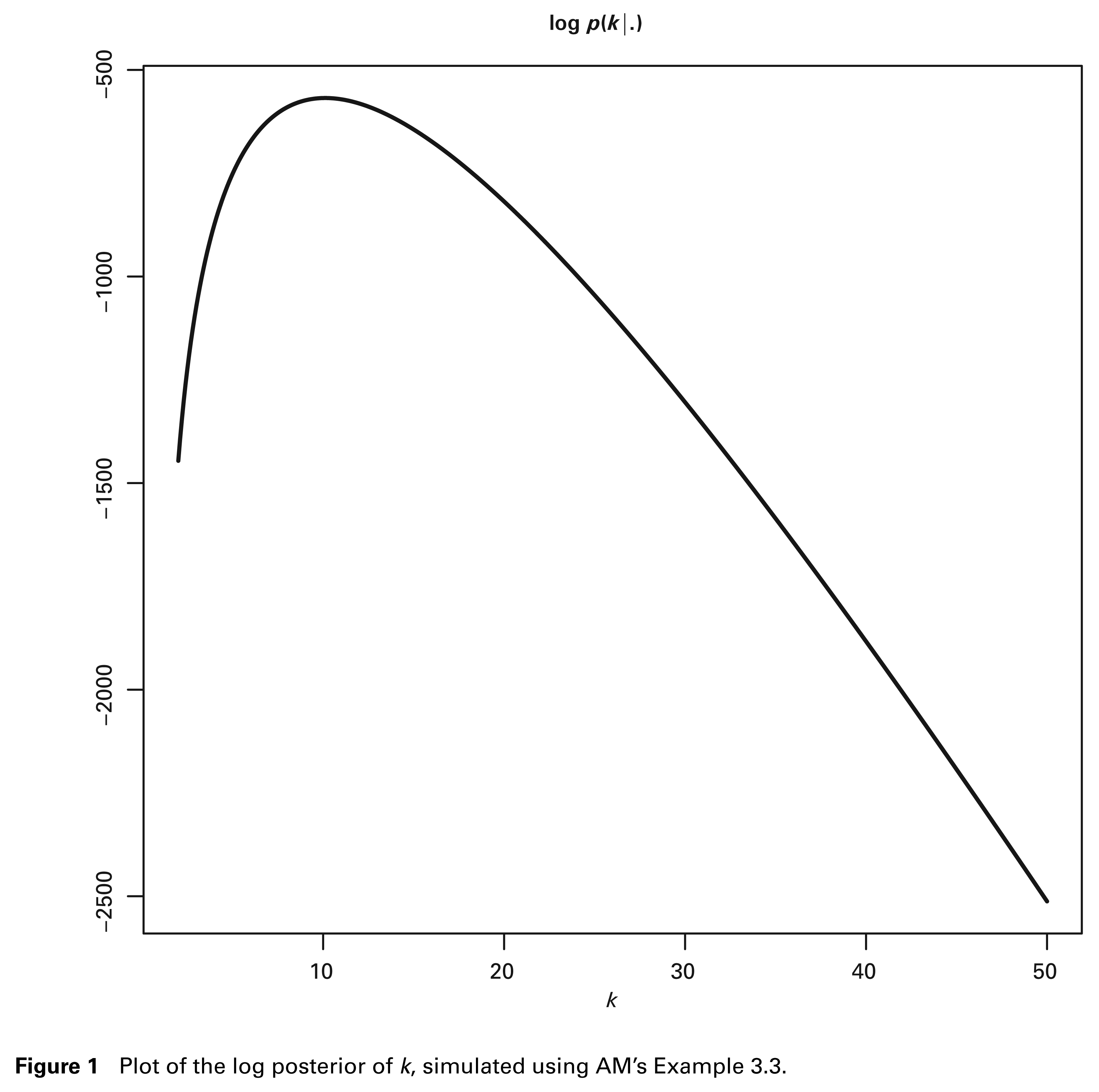
It is known that if the posterior density is assured to be log-concave, the adaptive rejection sampling (ARS) of Gilks (1992) can be more efficient than ARMS. Efficiency increases for two reasons. First, as the log-concavity is known, we no longer need to perform the additional point-evaluation of the log-density required by the call to the ARMS function. Second, we can construct the squeezing functions so that the function evaluation may be saved in each rejection step. Figure 1 shows the log posterior distribution function of k using the data simulated from the settings of AM’s Example 3.3. Clearly, the log density presents a concave shape, motivating the application of ARS in lieu of ARMS to improve computational efficiency. Here we emphasize that, in practice, switching from ARMS to ARS is cost-free, as most ARS and ARMS packages offer both options, for example, OX, R, WinBUGS and the C program by Gilks et al. (1995).

Figure 1

Plot of the log posterior of k, simulated using AM’s Example 3.3.

The following section discusses the log-concavity of the conditional posterior of k. We also apply Sherman-Morrison-Woodbury formula (SMW, see, e.g., Monahan, 2001) to reduce the computational burden during the update of the augmented latent covariance matrices. The utilization of ARS for k and SMW formula for the latent variables, taken together, form the basis of our sampling scheme that provides better computational efficiency.

3.1 The conditional posterior distribution of k

For the prior of k, PG consider the following gamma prior

π (k) \propto e x p {(α - 1) l o g k - λ_{0} k}, k > q,

where q is the dimension of the A matrix. AM adopt an exponential prior as given in Section 2.2. Notice that the two priors are equivalent if we set α = 1. Since PG’s prior distribution form is more general, the following discussion is based on PG’s setting. In practice, we set a vague prior by choosing α ≥ 1. Conditioned on the latent variables P _t , the log posterior density of k is obtained as follows:

\begin{array}{l} l o g p (k | \cdot) & \propto (α - 1) l o g k - λ_{0} k + \frac{T k}{2} (q l o g \frac{k}{2} - l o g | A |) - T \sum_{j = 1}^{q} l o g Γ (\frac{k + 1 - j}{2}) \\ + \frac{k}{2} \sum_{t = 1}^{T} l o g | P_{t - 1}^{d / 2} P_{t}^{- 1} P_{t - 1}^{d / 2} | - \frac{1}{2} t r [A^{- 1} C^{- 1} (k)] ​, \end{array}

where $\begin{array}{l} l o g p (k | \cdot) & \propto (α - 1) l o g k - λ_{0} k + \frac{T k}{2} (q l o g \frac{k}{2} - l o g | A |) - T \sum_{j = 1}^{q} l o g Γ (\frac{k + 1 - j}{2}) \\ + \frac{k}{2} \sum_{t = 1}^{T} l o g | P_{t - 1}^{d / 2} P_{t}^{- 1} P_{t - 1}^{d / 2} | - \frac{1}{2} t r [A^{- 1} C^{- 1} (k)] , \end{array}$ . The first-order derivative of the log posterior density is

\begin{array}{l} \frac{d}{d k} l o g p (k | \cdot) & = \frac{α - 1}{k} - λ_{0} + \frac{T q}{2} (l o g \frac{k}{2} + 1) - \frac{T}{2} l o g | A | - \frac{T}{2} \sum_{j = 1}^{q} ψ (z_{j}) \\ + \frac{1}{2} \sum_{t = 1}^{T} l o g | P_{t - 1}^{d / 2} P_{t}^{- 1} P_{t - 1}^{d / 2} | - \frac{1}{2} t r [A^{- 1} (\sum_{t = 1}^{T} P_{t - 1}^{d / 2} P_{t}^{- 1} P_{t - 1}^{d / 2})] ​, \end{array}

where ψ(•) is a digamma function and $z_{j} = \frac{k + 1 - j}{2}$ .

We then obtain the second-order derivative as:

\begin{array}{l} \frac{d^{2}}{d k^{2}} l o g p (k | \cdot) & = \frac{1}{4} T {q \frac{2}{k} - \sum_{j = 1}^{q} ψ_{1} (z_{j}) - \frac{α - 1}{k^{2}}} \\ \leq \frac{1}{4} T q {\frac{2}{k} - ψ_{1} (\frac{k}{2}) - \frac{α - 1}{q k^{2}}} . \end{array}

(3.1)

The inequality comes from the fact that the trigamma function ψ₁(x) is strictly decreasing in x. Accordingly, since $\frac{k}{2} \geq z_{j}$ for j = 1, …, q, we have $ψ_{1} (\frac{k}{2}) \leq ψ_{1} (z_{j})$ for all j ≥ 1. From the second line of Equation (3.1) we know that $- \frac{α - 1}{q k^{2}} \leq 0$ given α ≥ 1. Therefore, to complete the proof we only need to show that 2/k−ψ₁(k/2) ≤ 0. Taking x = k/2 > 0, and applying the inequality of Choi and Wette (1969),

ψ_{1} (x) = \sum_{i = 0}^{\infty} {(i + x)}^{- 2} > \int_{Z = 0}^{\infty} {(Z + x)}^{- 2} d Z = \frac{1}{x}, Z \geq 0,

the result immediately follows.

3.2 Use of Sherman-Morrison-Woodbury formula

In the MCMC estimation, we need to update the inverse covariance matrix whose conditional posterior is proportional to a Wishart distribution with the scale matrix

{\tilde{S}}_{t - 1} = {(S_{t - 1}^{- 1} + x_{t} x_{t}^{'})}^{- 1}, t = 1, \dots, T,

where x _t denotes the return vector in PG’s model and the standardized series in AM’s model, respectively. Applying SMW formula, the scale matrix ${\tilde{S}}_{t - 1}$ can be calculated by

{(S_{t - 1}^{- 1} + x_{t} x_{t}^{'})}^{- 1} = S_{t - 1} - \frac{S_{t - 1} x_{t} x_{t}^{'} S_{t - 1}}{1 + x_{t}^{'} S_{t - 1} x_{t}} .

Since in each sweep, S _t _–1 is known from the previous iteration, we can obtain ${\tilde{S}}_{t - 1}$ by a rank-1 update rather than by a matrix inversion from scratch. Obviously, this is computationally cheaper and hence should be incorporated into the WIC models as a general estimation strategy.

3.3 Comparison in computational efficiency

This section conducts a study using real data to show that our proposed scheme, denoted by ‘ARS+SMW’, is computationally more efficient than AM’s procedure, denoted as ‘ARMS+NoSMW’. Here the readers should be reminded that, in ‘ARS+SMW’, only k is sampled using ARS; for the other univariate parameter, d, following AM, we use ARMS to make draws. The raw data are collected from Yahoo Finance and consist of four series of weekly stock market indices, namely, the Dow Jones Industrial Average, the Hang Seng Index, the Korea Composite Stock Price Index and the Taiwan Weighted Stock Index. The sample period from 7 July 1997 to 9 November 2009 contains T = 452 observations. The returns are calculated by 100 × (log P_it – log P_i,t_–1), where P_it is the closing price on week t for stock market i. We fit the data with AM’s DC-MSV. Following AM, we first estimate the SV parameters and obtain the standardized series. After the pre-processing step, we estimate the correlation-level parameters for 20 times using ARS+SMW and ARMS+NoSMW, respectively. In each replication we run N = 30 000 MCMC iterations, with the first 10 000 draws discarded, and the remaining M = 20 000 are kept. The programs are written in OX (Doornik, 2007) Console 6.21 on a Windows7 platform, on a laptop equipped with an Intel i7 M620 2.67 GHz central processing unit and 4 GB random access memory. Note that we do not output the result for the SV part since the SV estimation stage is of no interest in the study.

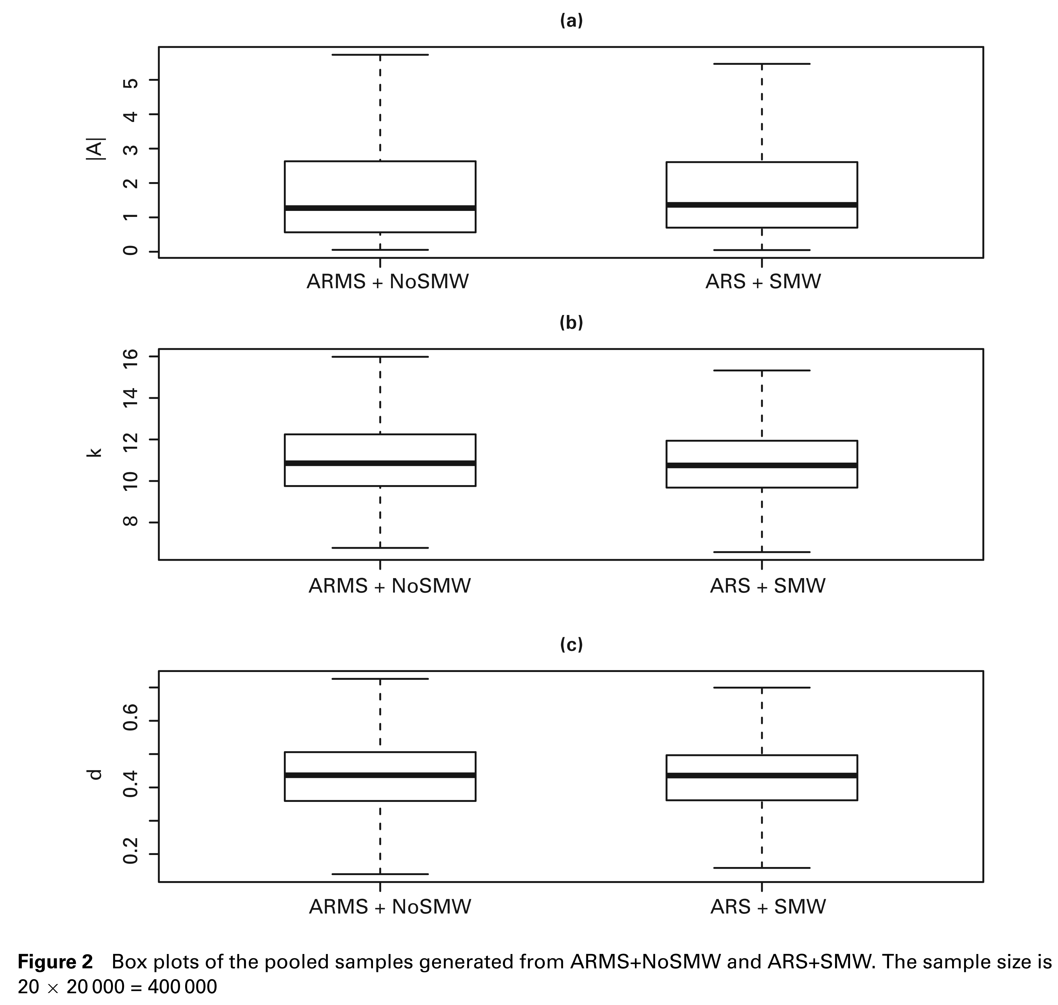
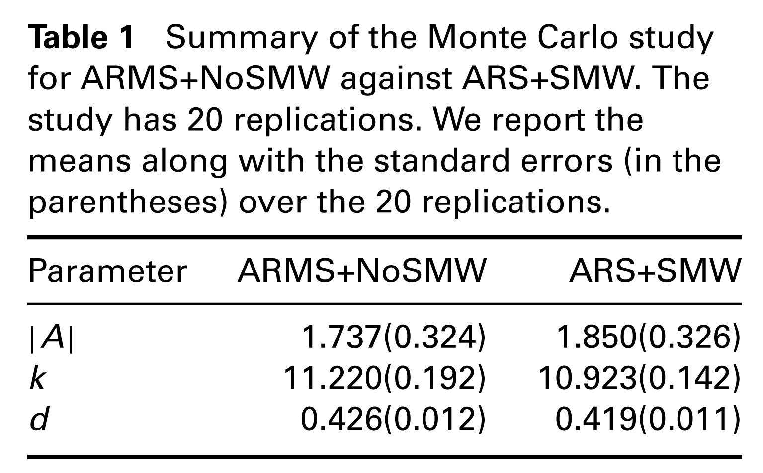
It is important to ensure that the samples generated from ARMS+NoSMW and ARS+SMW are comparable. To compare the posterior draws, for each method we pool all the MCMC draws together, generating a sample size of 20 × 20 000 = 400 000. Figures 2 (a), (b) and (c) show the box plots of | A |, k and d, respectively, where |•| denotes the determinant. We can see from Figure 2 that, for each parameter, the box plots appear to be nearly identical, suggesting that the sample distributions are similar. Table 1 summarizes the Monte Carlo study over the 20 replications. We report the means along with their standard errors (in the parentheses). It is clear that the two samplers produce very similar results.

Figure 2

Box plots of the pooled samples generated from ARMS+NoSMW and ARS+SMW. The sample size is 20 × 20 000 = 400 000

Table 1

Summary of the Monte Carlo study for ARMS+NoSMW against ARS+SMW. The study has 20 replications. We report the means along with the standard errors (in the parentheses) over the 20 replications.

Parameter	ARMS+NoSMW	ARS+SMW
\|A\|	1.737(0.324)	1.850(0.326)
k	11.220(0.192)	10.923(0.142)
d	0.426(0.012)	0.419(0.011)

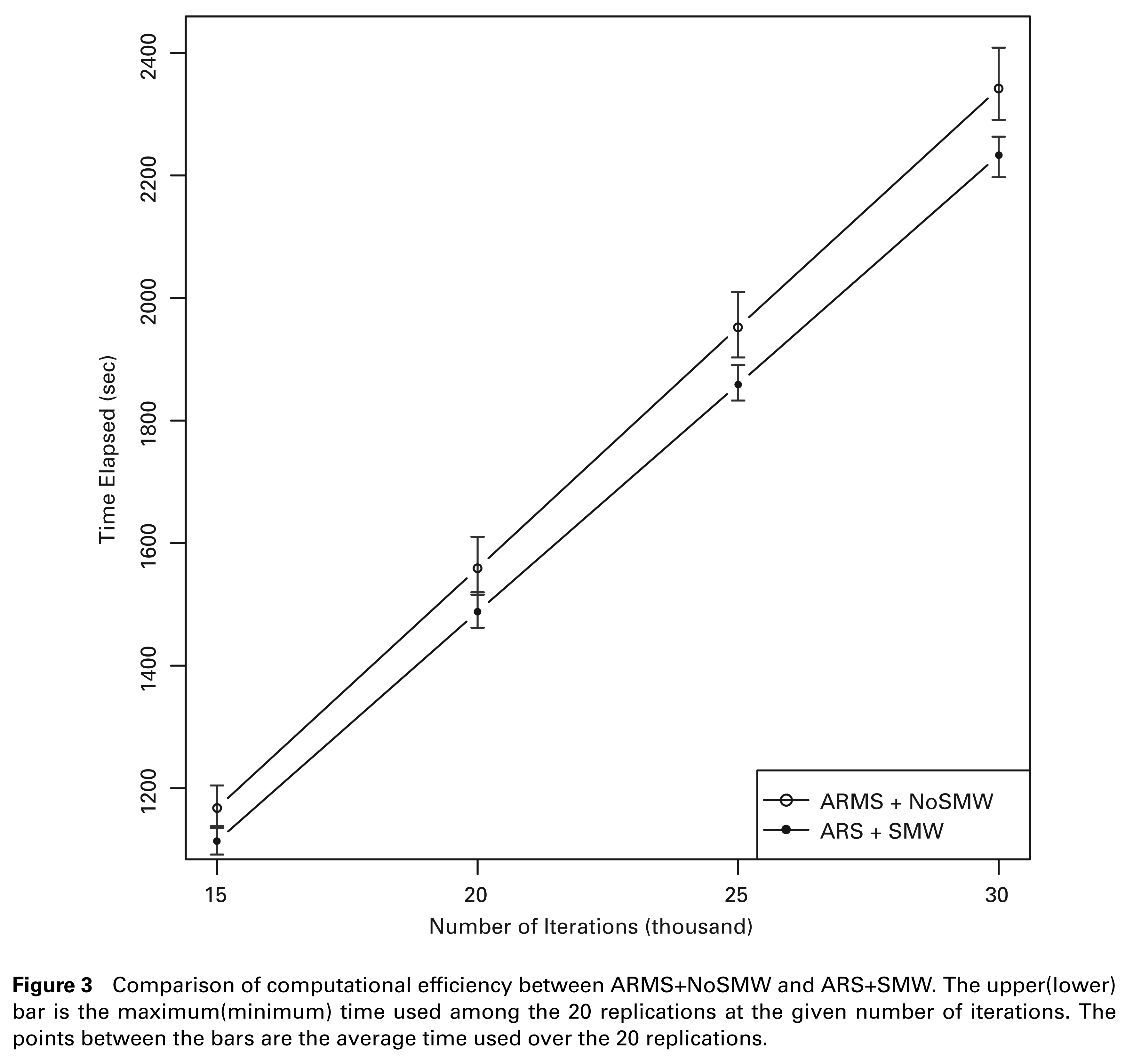
To compare computational efficiency, in each replication we record the time elapsed at n = 15 000, 20 000, 25 000, and 30 000 iterations, and for each n, we find the minimum, average and maximum values among the 20 replications. Figure 3 shows the results. It is interesting to first note that the increase of the running time against the number of iterations is larger for ARMS+NoSMW than for ARS+SMW. Hence, although the minimum–maximum time intervals overlap for n ≤ 20 000, in the end they become disjoint. The result not only presents strong evidence that ARS+SMW is more efficient, but it also indicates that ARS+SMW can be even more advantageous if more MCMC iterations are required. At n = 30 000, where one single MCMC is completed, the average time taken by ARMS+NoSMW(ARS+SMW) is 2 341.9(2 225.4) seconds, showing that ARS+SMW improves the computational efficiency by 5.2%. This can be a considerable saving of time in some practical use, especially when we need to conduct the estimation procedure for multiple times. It is also of our interest to evaluate the contribution from SMW formula alone. We conduct the same experiment for the combination ‘ARMS+SMW’ and compare it with ARMS+NoSMW. The average time to complete a replication with ARMS+SMW is 2 287.4 seconds, indicating that the use of SMW formula saves about 2.4% in running time.

4 Empirical study

In this section we provide an example of how DCFMSV works and compare it with three existing volatility models, namely, AM’s DC-MSV, PG’s diagonal idiosyncratic covariance matrix FMSV model (see equation (9) in PG) and the well-known DCC-GARCH, which belongs to the family of GARCH-type volatility models. It should be emphasized that our purpose is to compare the predictive performance rather than to illustrate more applications. PG have used real data to demonstrate how the WIC FMSV model can be applied to out-of-sample portfolio optimization.

Figure 3

Comparison of computational efficiency between ARMS+NoSMW and ARS+SMW. The upper(lower) bar is the maximum(minimum) time used among the 20 replications at the given number of iterations. The points between the bars are the average time used over the 20 replications.

4.1 The data

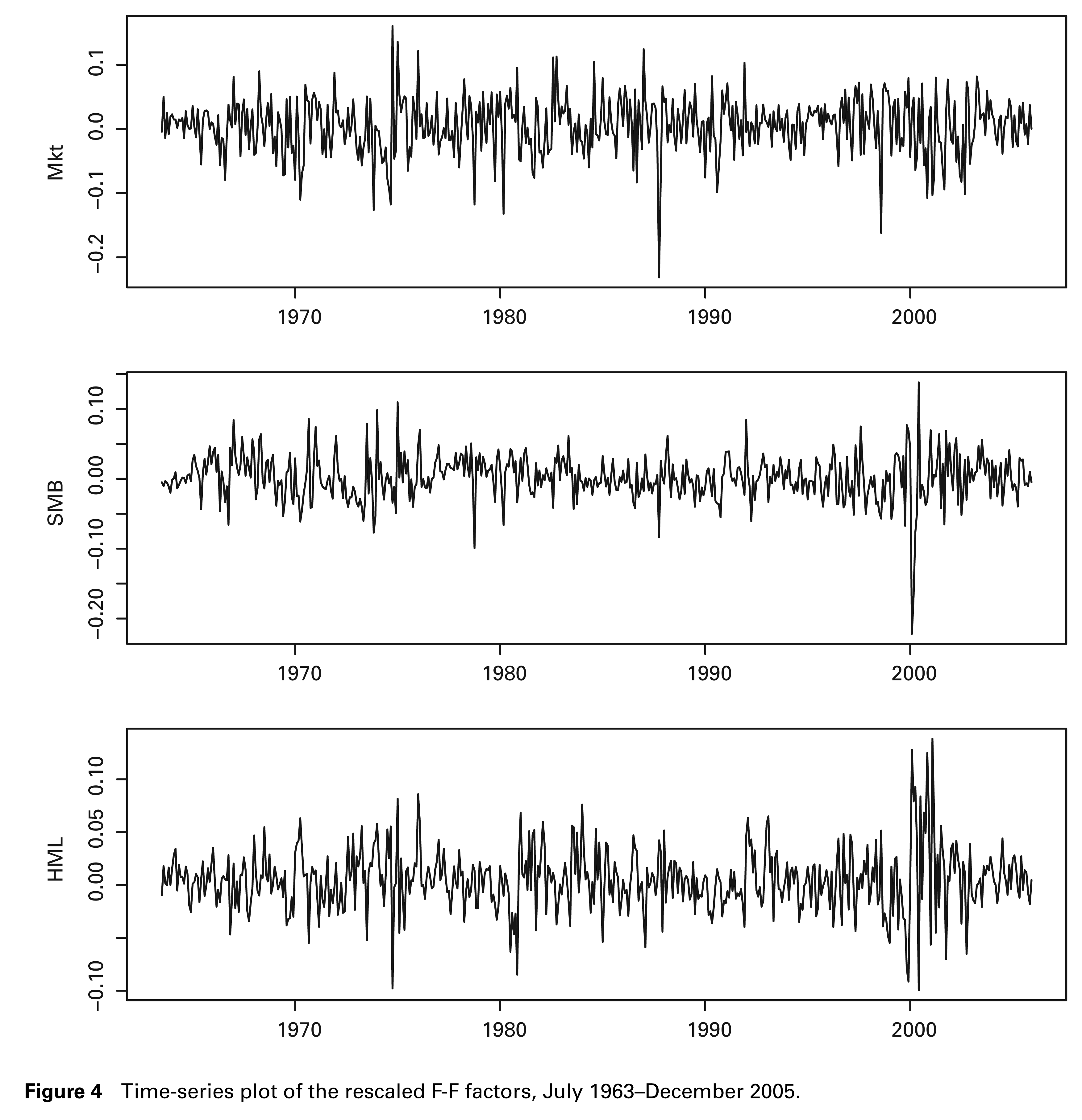
The example is illustrated with monthly data. We choose three Fama-French (F-F) factors: the market excess return (MKT), the Small-Minus-Big (SMB) and the High-Minus-Low (HML) factors. The return series are the average value weighted returns for 10 industry portfolios. The 10 portfolios are NoDur, Durbl, Manuf, Enrgy, HiTec, Telcm, Shops, Hlth, Utils and Other. We obtain the factors and returns from Dr. Kenneth French’s data library. The observation period is from July 1963 to December 2005 with a total sample size of 510. A detailed description for these data can be found in the data library. All data are converted to a (−1,1) scale by multiplying by 0.01. Figure 4 shows the time-series plots of the three rescaled F-F factors. As can be seen clearly, the factor volatilities have quite different patterns. The heterogeneity in factor volatilities suggests that permitting the factors to have separate SV processes is helpful in describing the dynamics.

4.2 Model comparison

The specification of AM’s DC-MSV is identical to settings (2.2a)–(2.5). For PG’s FMSV model, we have the following specification:

\begin{array}{l} y_{t} | B, f_{t}, Ω \sim N_{p} (B f_{t}, Ω), \\ f_{t} | P_{t} \sim N_{q} (0, P_{t}), \\ P_{t}^{- 1} | P_{t - 1}^{- 1}, S_{t - 1} \sim W_{q} (P_{t - 1}^{- 1} | k, S_{t - 1}), \end{array}

where the matrix P _t is a factor covariance matrix, the meaning of the matrix A and the scalar parameters d and k are the same as those in DCFMSV. For the DCC-GARCH model, we adopt the parameterization of Engle (2002) and specify the orders (1,1) and Gaussian errors for each univariate series. We estimate the parameters and forecast future observations using the R package ‘rmgarch’ developed by Ghalanos (2012). Following Geweke and Amisano (2010), the model performance is evaluated with the cumulative log predictive Bayes factor. The calculation of the predictive density for DCC-GARCH is straightforward. For the MSV class of models, we use a Monte Carlo integration to approximate the posterior predictive density

p (y_{t + 1} | ℱ_{t}; ℳ) = \int^{​} p (y_{t + 1} | ℱ_{t}, θ_{ℳ}; ℳ) p (θ_{ℳ} | ℱ_{t}; ℳ) d θ_{ℳ},

where M is the specific model, F_t is the information collected up to time t and θ_M is the set of parameters for M. The cumulative log predictive Bayes factor of Model 1 against Model 0 is calculated by

l o g (B_{1, 0}) = \sum_{t} l o g p (y_{t} | ℱ_{t - 1}; ℳ_{1}) - \sum_{t} l o g p (y_{t} | ℱ_{t - 1}; ℳ_{0}) .8

Kass and Raftery (1995) suggest the log scoring rule for the evaluation of model predictive quality: if log(B_1,0) < 0, the evidence is in favour of Model 0; if log(B_1,0) ∈ [0, 1), the evidence is not worth more than a bare mention; if log(B_1,0) ∈ [1, 3), the evidence is positively in favour of Model 1; if log(B_1,0) ∈ [3, 5), the evidence is strongly in favour of Model 1; if log(B_1,0) > 5, we have very strong evidence in favour of Model 1. The out-of-sample prediction period is three-year long, from January 2006 to December 2008, with a total length N = 36. This time frame covers two market conditions: a relatively calm market before 2007, and the post-2007 period with a relatively volatile market due to the subprime crisis, in which we can compare model performance across different market conditions. The one-step-ahead prediction is conducted on a rolling basis, that is, if we use observations y ₁, …, y _T to forecast y _T ₊₁, then in next period, y _T ₊₁ is included as a sample for the prediction of y _T ₊₂. In the MCMC procedure we take N = 30 000 and M = 20 000.

Figure 4

Time-series plot of the rescaled F-F factors, July 1963–December 2005.

Table 2

Results for the comparison of DCFMSV (DCF) against AM’s DC-MSV (AM), PG’s FMSV (PG) and DCC-GARCH (DCC) based on the cumulative log predictive Bayes factor

Measure	Value
log (B_DCF,AM)	241.54^a
log (B_DCF,PG)	14.94
log (B_DCF,DCC)	12.83

Note: ^aThe time frame of the comparison does not include October 2008.

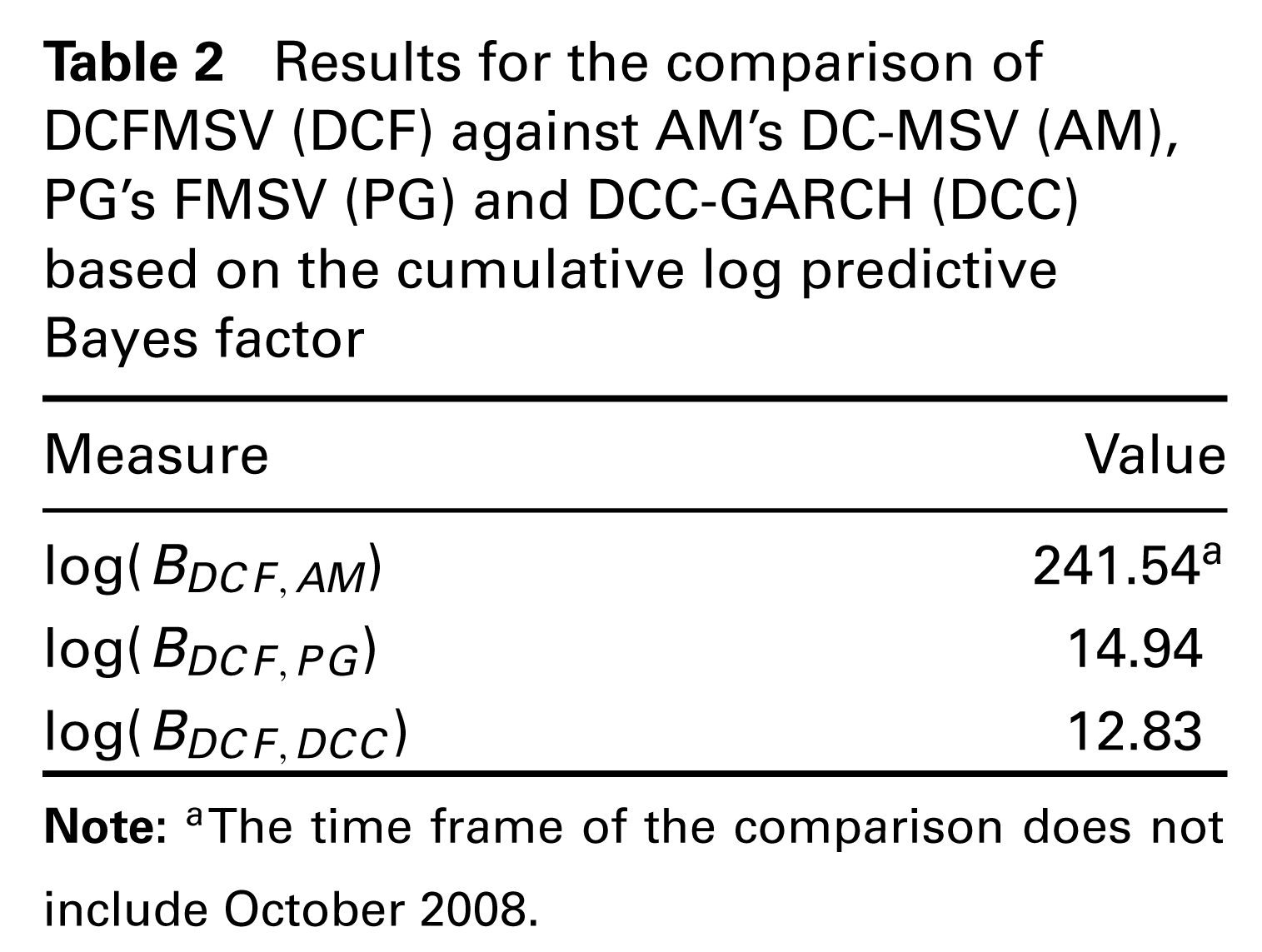
Table 2 summarizes the results. The values log(B_DCF,AM), log(B_DCF,PG) and log(B_DCF,DCC) are the cumulative log predictive Bayes factor of DCFMSV against AM’s DC-MSV, PG’s FMSV and DCC-GARCH, respectively. Contrary to our expectation, the first result suggested by log(B_DCF,AM) indicates that DC-MSV performs much worse than its ‘factored’ version, DCFMSV. This result may not be surprising. As we point out in the introduction, since the whole large dependence structure is governed by simply one scalar parameter d, all the 55 elements have to compromise with each other to some extent. Moreover, DC-MSV performs particularly poorly in turbulent periods. For October 2008, the month right after the bailout of Fannie Mae and Freddie Mac, the predictive likelihood under DC-MSV is not even available because the value is smaller than the minimum value representable by the software package. In addition to the poor predictive quality, the rapid increase in computational cost makes DC-MSV unfavourable to work with. The running time of DC-MSV on the 10-dimensional data is more than seven times as much as that of DCFMSV with three factors. From both perspectives we argue that DCFMSV is more suitable than DC-MSV when the dimension of data is large. The other results in Table 2 show the superiority of DCFMSV over PG’s FMSV and the DCC-GARCH model.

The empirical study offers another chance to compare the computational efficiency. We utilize both ARMS+NoSMW and ARS+SMW to estimate DCFMSV. The running time taken by ARMS+NoSMW (ARS+SMW) is 85 960 (82 438) seconds, showing that ARS+SMW saves almost 1 hour, which we believe is quite favourable for practitioners. Notice that, compared to the result of the Monte Carlo study in Section 3.3, here the improvement by ARS+SMW is reduced to 4.2%. This is because the augmented factor covariance matrix is only of dimension 3, and consequently, SMW formula makes limited contribution. Figure 5 is the plot of the running time for each forecasting period. It is readily seen that the time curve of ARS+SMW is uniformly below that of ARMS+NoSMW. Moreover, the running time increases as the time frame expands, and the difference between the two time curves is enlarged. The pattern implies that, for the applications that require repeated estimation, the use of ARS+SMW is even more favourable.

We close this section with the discussion on the choice of the number of factors, which is an important issue that is not explored in PG. To deal with the model selection problem, we suggest a straightforward solution utilizing the cumulative log predictive Bayes factor. For example, suppose we want to select between the three-factor (full) model and the two-factor (reduced) model which contains the pair of factors (MKT, SMB). We calculate and obtain log(B_{Reduced, Full}) = 5.82 > 5, by which we would select the two-factor model since it provides a better fit to the data.

Figure 5

Comparison of computational efficiency between ARMS+NoSMW and ARS+SMW using real data.

5 Conclusion and discussion

This article proposes a flexible dynamic-correlation FMSVmodel in which the factors are observable. The novelty of the model is its ability to simultaneously allow the factors to have separate SV processes and the factor covariance matrices to follow an inverse Wishart process. To estimate the model, we develop a computationally efficient method based on Bayesian MCMC algorithms. The method makes two contributions to the WIC literature. First, it substantially improves the computational efficiency of MCMC sampling. Second, forecasting can be carried out with the algorithm, which in turn provides a solution to the choice of the number of factors. These improvements to a great extent broaden the scope of the WIC model applications. The result of the model comparison based on predictive quality shows that DCFMSV outperforms all other competing models, including AM’s DC-MSV, PG’s FMSV and DCC-GARCH.

In DCFMSV we can as well apply a latent factor structure, where the factors need to be estimated. However, because of the well-known nonidentifiability problem, some constraints such as the lower triangular condition on the loading matrix must be imposed (see, for example, Geweke and Zhou, 1996; Lopes and West, 2004). Concern arises when applying this type of constraints, in view of the fact that the zero structure on the upper triangle blocks the channels through which the factors come into the system. As a result, the first series y _1t can only take the first factor into account, and the second series y _2t can only take the first two factors, and so on, which clearly causes loss of generality. Other types of constraints, for example, the orthogonality constraint on the latent factors, may also be problematic as PG point out in their discussion. Modelling the evolution of the time-varying correlations via latent factors, therefore, can lead to loss of some desirable features of the current model. Although, for this reason, we only consider observable factors, we do believe that incorporating latent factors into the WIC MSV models is worth of future studies.

Footnotes

Acknowledgements

The author is grateful to Professor Robert Kohn at the University of New South Wales, Sydney, Australia, for his valuable comments on the article.

References

Asai

McAleer

(2009) The structure of dynamic correlations in multivariate stochastic volatility models. Journal of Econometric, 150, 182–92.

Chib

Nardari

Shephard

(2006) Analysis of high dimensional multivariate stochastic volatility models. Journal of Econometrics, 134, 341–71.

Choi

Wette

(1969) Maximum likelihood estimation of the parameters of the gamma distribution and their bias. Technometrics, 11, 683–90.

Doornik

(2007) Object-oriented matrix programming using Ox. London and Oxford: Timberlake Consultants Press, 3 edition www.doornik.com.

Engle

(2002) Dynamic conditional correlation: A simple class of multivariate generalized autoregressive conditional heteroskedasticity models. Journal of Business and Economic Statistics, 20, 339–50.

Geweke

Amisano

(2010) Comparing and evaluating bayesian predictive distributions of asset returns. International Journal of Forecasting, 26, 216–30.

Geweke

Zhou

(1996) Measuring the pricing error of the arbitrage pricing theory. Review of Financial Studies, 9, 557–87.

Ghalanos

(2012) rmgarch: multivariate GARCH models, Version 0.97.

Gilks

(1992) Derivative-free adaptive rejection sampling for gibbs sampling. In Bernardo

Berger

Dawid

Smith

AFM

editors, Oxford: Oxford University Press, Bayesian Statistics, volume 4, pp. 169–93.

10.

Gilks

Best

Tan

KKC

(1995) Adaptive rejection metropolis sampling within gibbs sampling. Journal of the Royal Statistical Society. Series C (Applied Statistics), 44(4), 455–72. ISSN 00359254. http://www.jstor.org/stable/2986138.

11.

Harvey

Ruiz

Shephard

(1994) Multivariate stochastic variance models. Review of Economic Studies, 61, 247–64.

12.

Jacquier

Polson

Rossi

(1995) Models and prior distributions for multivariate stochastic volatility. Technical Report 95-18, CIRANO: Scientific Series, Montreal.

13.

Kass

Raftery

(1995) Bayes factors. Journal of American Statistical Association, 90, 773–95.

14.

Kim

Shephard

Chib

(1998) Stochastic volatility: likelihood inference and comparison with arch models. Review of Economic Studies, 65, 361–93.

15.

Liesenfeld

Richard

J-F

(2006) Classical and Bayesian analysis of univariate and multivariate stochastic volatility models. Econometric Reviews, 25, 335–60.

16.

Liu

(2001) Monte carlo strategies in scientific computing. Springer-Verlag.

17.

Lopes

Carvalho

(2007) Factor stochastic volatility with time varying loadings and Markov switching regimes. Journal of Statistical Planning and Inference, 137, 3082–91.

18.

Lopes

West

(2004) Bayesian model assessment in factor analysis. Statistica Sinica, 14, 41–67.

19.

Monahan

(2001) Numerical methods of statistics. Cambridge: Cambridge University Press.

20.

Philipov

Glickman

(2006a) Multivariate stochastic volatility via wishart processe. Journal of Business and Economic Statistics, 24, 313–28.

21.

Philipov

Glickman

(2006b) Factor multivariate stochastic volatility via Wishart processes. Econometric Reviews, 25, 311–34.

22.

Pitt

Shephard

(1999) Time-varying covariances: a factor stochastic volatility approach. In Bernardo

Berger

Dawid

Smith

AFM

, editors, Bayesian statistics, volume 6, pp. 169–93. Oxford: Oxford University Press.