Modelling of overall survival by an association between progression-free and post-progression survival using a conditional distribution

Abstract

In oncology, overall survival (OS) is the optimal endpoint for measuring the clinical benefit. However, and contrary to progression-free survival (PFS) which represents a potential surrogate endpoint of OS in clinical trials, OS often requires a long follow-up where the effect of the studied treatment may be diluted by subsequent therapies. In the literature, the relationship between PFS and OS was investigated more analytically than theoretically. We propose a new statistical modelling for OS based on the two survival times: PFS and post-progression survival (PPS) which we assumed to be linked using a conditional exponential distribution. This model allows us to test the existence of an association between PFS and PPS to better understand the process of improvement or decrement of OS. We found a closed form of the correlation coefficient between PFS and both PPS and OS. We expressed them as simple formulas in function of model parameters. One of the model parameters proved to be a correlation indicator between these survival times. We also defined the likelihood of the model in order to use the maximum likelihood estimator to estimate the model parameters from Phase III randomized clinical trial data, involving patients with locally advanced non-small cell lung cancer. The results showed a significant link between PFS and PPS and a strong association between improvements in PFS and OS.

Keywords

Oncology overall survival parametric modelling post-progression survival progression-free survival

1 Introduction

In oncology studies, clinical trials are carried out to assess the effect and confirm the effectiveness of an intervention, an experimental drug or treatment using clinical endpoints measured, generally based on the time of occurrence of an event and more specifically on the survival time. The US Food and Drug Administration (FDA) considers overall survival (OS) as the most reliable cancer endpoint to measure the clinical benefit. According to US FDA (2007) guidelines, OS is defined as the time from randomization until death from any cause. Indeed, OS considers all forces of mortality related or not to the disease of interest. For example, cancer patients face death from their cancer and also from other life-threatening situations, such as, the toxicity of the cancer therapy itself, other diseases and accidents. OS is based on the accurate statistic of date of death and is therefore easy to measure and clinically significant. However, as OS often requires lengthy and expensive clinical trials, it is not easy to conclude that an experimental treatment improves survival or not. Indeed, to approve drug efficiency or to detect treatment differences, it is necessary to monitor a considerable number of patients over a long period. That is why it is interesting to substitute OS by a valid clinical surrogate endpoint to mesure the effect of treatment after a relatively short period of time.

There are several clinical criteria that have been used to approve the effectiveness of treatment. These criteria are based on tumour assessments such as response rate that is not a time-to-event endpoint, time-to-progression (TTP) and progression-free survival (PFS). Note that a precise and detailed definition of tumour progression based on the RECIST, (Therasse et al., 2000; Eisenhauer et al., 2009) amendments is essential in the protocol. The FDA has defined PFS as the time elapsed between randomization and tumour progression or death from any cause. On the other hand, TTP is defined as the time from randomization to tumour progression where deaths occurred before progressions were censored which is not the same functional aspect as in PFS. Porzsolt et al. (2009) showed that TTP overestimates treatment effects and so it is more appropriate to use PFS as a surrogate of OS. By considering PFS as a primary endpoint, the FDA has recently approved several new cancer drugs. While there is no formal validation of PFS as a surrogate endpoint in advanced breast cancer (Burzykowski et al., 2008; Saad et al., 2010), PFS formally became a valid primary endpoint for colorectal cancer (Buyse et al., 2007; Tang et al., 2007). S. Singh and C. Law (2010) reported that the use of PFS as an endpoint in neuroendocrine tumour clinical trials may facilitate the evaluation, approval and development of new treatments.

At first sight, PFS seems to be the most suitable substitute for OS because it requires follow-up only until tumour progression. As rightly pointed out by Dr Daniel J. Sargent, a biostatistician within the North Central Cancer Treatment Group, in an article (Mayfield, 2008) ‘Most patients stop taking the study drug when their disease begins to progress, so the PFS clock stops at that point.’ Because PFS reduces the duration of clinical trials, the experimental treatment effect cannot be confounded by subsequent therapies. Furthermore, PFS includes death and thus the relationship between PFS and OS can be an even better correlation. If in fact there is a positive correlation between PFS and OS, it suggests that improvement in PFS leads to improvement in OS and so PFS may be an appropriate potential surrogate. In order to provide a surrogate endpoint for OS, several authors have empirically investigated the correlation between OS and other clinical criteria especially PFS (see Louvet et al., 2001; Ballman et al., 2007; Sherrill et al., 2007; Burzykowski et al., 2008; Lamborn et al., 2008; Foster et al., 2011; Heng et al., 2011; Hurvitz, 2011).

Despite the use of correlation approach as a statistical method in the majority of studies and the importance of PFS as a potential surrogate endpoint in the development of new anti-cancer treatments, there are few studies on parametric approaches that characterize OS and its association with PFS. Assuming an appropriate distribution for survival times, it is possible to introduce explanatory variables in the functions of risk. By taking into account more information, the estimators obtained are more efficient than the nonparametric estimators as the Kaplan and Meier (1958) estimator, and this is one of the main advantages of the parametric approaches. Begg and Larson (1982) used a parametric model where the time to tumour progression or to death was assumed to be exponential. Building on this work, Ellis et al. (2008) used other time-to-event distributions than the simple exponential such as Weibull and log Normal. Fleischer et al. (2009) developed a statistical model of OS based on exponential distributions assuming a dependency between TTP and OS. Moreover, continuous-time multi-state models are a useful way of describing medical processes allowing patients to move from one state to another, for example, from disease-free state to death state. The progressive three-state model and the illness–death model are the most commonly used three-state model. In the Markov model, the transition intensity which represents the instantaneous risk of moving from one state to another depends only on the current state. There are different models regarding the dependance of the transition intensity. First, the time-homogeneous Markov model allows transition probabilities to be found in closed form using Kolmogorov’s forward equations (Cox and Miller, 1965) where the transition intensities are assumed to be constant as functions of time. In addition, a time non-homogeneous Markov model is needed in cases where the transition intensities vary through current time. Non-homogeneous Markov processes may be modelled parametrically by assuming piecewise constant transition intensities (Perez-Ocon et al., 2001) or nonparametrically using the Aalen–Johansen estimator for the estimation of the state occupation probabilities (Aalen and Johansen, 1978). However, the Markov property may be inappropriate and may lead to biased estimates. It should be noted that Datta and Satten (2001) showed the consistency of the Aalen–Johansen estimator even when the multi-state model was not Markov. Another approach is to use the semi-Markov model in which the transition intensities not only depend on current time, but also on the duration in current state (Andersen and Keiding, 2002). Finally, avoiding the Markov property, Pepe (1991), Strauss and Shavelle (1998) and Meira-Machado et al. (2006) proposed nonparametric estimators for the probability of state occupation based on the proportion of censored and uncensored patients in each state.

In this article we propose an alternative parametric modelling for OS that is easy to understand and to implement. The proposed model generalizes the structure of dependency between PFS and OS. The rest of this article is organized as follows. The approach is described in Section 2 by generalizing the main functions which are useful for modelling. In Section 3, the general form of model likelihood is given. Section 4 presents the proposed model, the obtained correlation coefficients and also the use of covariates. Section 5 presents an application to data from a randomized Phase III clinical trial involving patients with locally advanced non-small cell lung cancer. In conclusion, there is a discussion in Section 6.

2 General model

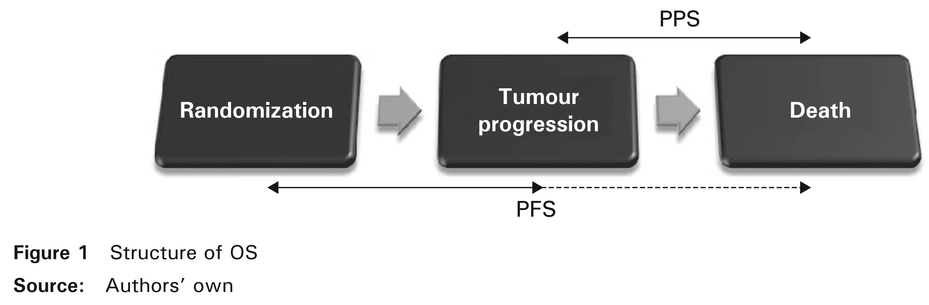
As indicated in Figure 1, if tumour progression and death have been observed then OS includes two consecutive survival times before and after progression, PFS and post-progression survival (PPS). PPS is defined as the time elapsed between tumour progression (relapse) and death. If death is the only event observed, by definition, it is regarded as a progression and therefore PFS ≤ OS. The purpose of this section is to generalize the distribution of OS that we consider to be the sum of two assumed dependent survival times, PFS and PPS.

We start with a random experiment that has a sample space R^ and a probability measure P on R^. Suppose that T, X and Y are survival times for the experiment, where T represents OS, X is PFS and Y is PPS. These survival times take as values t, x and y respectively. We assume that X and Y could be statistically dependent. Since T = X + Y, F_T, the distribution function of T, is defined as follows:

F_{T} (t) = \int_{0}^{t} F_{Y | X} (t - x | x) f_{X} (x) d x,

where f_X is the density of X and F_Y_|X is the conditional distribution function of Y at y given X = x.

By deriving F_T(t) with respect to t, we found f_T, the density of T

f_{T} (t) = \int_{0}^{t} f_{Y | X} (t - x | x) f_{X} (x) d x,

where f_Y_|X is the conditional density of Y at y given X = x.

Given that S_T(t) = 1 – F_T(t), we deduced S_T, the survival function of T

S_{T} (t) = S_{X} (t) + \int_{0}^{t} S_{Y | X} (t - x | x) f_{X} (x) d x,

where S_X is the survival function of X and S_Y_|X is the conditional survival function of Y at y given X = x.

Figure 1

Source: Authors’ own

Moreover, S_Y, the survival function of Y is

S_{Y} (y) = \int_{0}^{\infty} S_{Y | X} (y | x) f_{X} (x) d x,

and the expectation of T is obtained as follows:

E (T) = \int_{0}^{\infty} S_{T} (t) d t

= E (X) + \int_{0}^{\infty} {\int_{x}^{\infty} S_{Y | X} (t - x | x) d t} f_{X} (x) d x

= E (X) + \int_{0}^{\infty} E (Y | X) f_{X} (x) d x

where EYE_XYX

3 Model likelihood

In order to estimate the model parameters, we used the maximum likelihood estimator (MLE). Based on the general form of the likelihood described by Yuan et al. (2011), we constructed the likelihood of our model by a factorization of five categories representing the eventual contributions of the likelihood for each patient.

Let N be the sample size and n_j_{(j = 1,...,5)} be the number of patients in each category,

n_{j} = \sum_{i = 1}^{N} 1_{(δ_{i} = j)},

where, for the ith patient, we define δ_i_{(i = 1,...,N)} as the categorical indicator, stated as follows:

For δ_i = 1, tumour progression and death were both observed and so the total likelihood contribution in this category is

L_{1} = \prod_{i = 1}^{n_{1}} f_{X} (x_{i}) f_{Y | X} (y_{i} | x_{i}),

where y_i = t_i – x_i.

For δ_i = 2, only tumour progression was observed and therefore death is censored. Let C be the administrative right censoring time which is assumed to be independent of survival times. Conditionally to x_i, y_i and $y_{i}^{c} = c_{i} - x_{i}$ are independent and thus the total likelihood contribution is

L_{2} = \prod_{i = 1}^{n_{2}} f_{X} (x_{i}) S_{Y | X} (y_{i}^{c} | x_{i}) .

If death occurred while tumour progression had not been yet observed, we have two possible likelihood contributions according to cause of death information:

For δ_i = 3, if the observed death was related to cancer, either directly or indirectly, then the total likelihood contribution in this case becomes

L_{3} = \prod_{i = 1}^{n_{3}} {1 - S_{X} (t_{i})} f_{T} (t_{i}),

because it is much more reasonable to assume that an undiagnosed relapse occurred either before or at the time of the observed cancer death (X ≤ t).

Otherwise, for δ_i = 4, the observed death was due to causes other than cancer. In that case, relapse is censored and the total likelihood contribution is

L_{4} = \prod_{i = 1}^{n_{4}} S_{X} (t_{i}) f_{T} (t_{i}) .

Finally, for δ_i = 5, neither tumour progression nor death were observed. Patients alive at the end of follow-up and lost to follow-up are censored. Then, the total likelihood contribution is

L_{5} = \prod_{i = 1}^{n_{5}} S_{X} (c_{i}) S_{T} (c_{i}) .

Therefore, the likelihood of the model is

L = \prod_{j = 1}^{5} L_{j} .

4 Proposed model

Based on the reasoning of Section 2 and the fact that the dependence structure between X and Y is represented by the conditional distribution of Y given X, we considered X and Y | X to be exponentially distributed with parameters λ and θ(x) respectively. Regarding the choice of θ(x), we preferred the flexible exponential form because it allows for analytical computation of the correlation coefficients, ease of parameter interpretation and potential goodness of fit.

For β and ν in R, we define

θ_{Y | X} (x) = α \exp (- β x), where α = \exp (ν) and β < λ / 2.

Hence, the hazard function of Y is

h_{Y} (y) = \frac{\int_{0}^{\infty} θ_{Y | X} (x) g (x, y) d x}{\int_{0}^{\infty} g (x, y) d x}

and the mortality fonction of T is

h_{T} (t) = \frac{\int_{0}^{t} θ_{Y | X} (x) g (x, t - x) d x}{\frac{\exp (- λ t)}{λ} + \int_{0}^{t} g (x, t - x) d x},

where g(x, y) = exp{–[θ_Y_|X(x)y + λx]}.

4.1 Measure of the association strength

In clinical studies, the validity of surrogate endpoints is an extremely important concept which remains fairly complex and poorly understood. Prentice (1989) established criteria to validate surrogate endpoints. These criteria essentially require that the surrogate and the true endpoints correlate. In cases where a death is related to tumour progression, there is a causal connection which most probably involves a correlation between X and T. We therefore determined correlation coefficients in order to measure the magnitude of this possible association.

First, we found the expectations of Y and T

E (Y) = \frac{λ}{α (λ - β)}

and

E (T) = \frac{λ^{2} + α (λ - β)}{α λ (λ - β)} .

Therefore, the covariances between X and Y and also between X and T are

Cov (X, Y) = \frac{β}{α {(λ - β)}^{2}}

and

Cov (X, T) = \frac{(α + β) λ^{2} - 2 α β λ + α β^{2}}{α λ^{2} {(λ - β)}^{2}} .

Correlation coefficient is based upon the covariance between the survival times that is a measure of how these variables change in relation to each other. So, technically the parameter β represents a correlation indicator that reveals the direction of the relationship between X and Y as well as between X and T. We noted that:

If β = 0, then Cov(X, Y) = 0 and Cov(X, T) = 1/λ². In this case, survival times X and Y are uncorrelated, where Y follows an exponential distribution with a rate parameter α.

If β > 0, then Cov(X, Y) and Cov(X, T) are positive. Thus, X and T (or Y) evolve in the same direction. In other words, for each increase in X compared to its average, we have an increase in T (or Y) compared to its average, and for every decrease in X, we have a decrease in T (or Y).

f –α ≤ β < 0, then Cov(X, Y) is negative and Cov(X, T) is positive. This means (unlike X and Y) that X and T are positively correlated. It is not uncommon to observe a significant increase in X that offsets the decrease in Y and thus obtaining an increase in T.

If β < –α, then Cov(X, Y) is negative and Cov(X, T) is null for $λ = λ' = β (α + \sqrt{- α β}) / (α + β)$ , positive for 0 < λ < λ′ and negative otherwise. In the case where both covariances are negative, for each decrease in X compared to its average we have an increase in T compared to its average, and inversely. For Cov(X, T) = 0, X and T are uncorrelated.

Further, we calculated variances of Y and T

Var (Y) = \frac{λ {{(λ - β)}^{2} + β^{2}}}{α^{2} {(λ - β)}^{2} (λ - 2 β)}

and

Var (T) = \frac{1}{λ^{2}} + \frac{λ {{(λ - β)}^{2} + β^{2}} + 2 α β (λ - 2 β)}{α^{2} {(λ - β)}^{2} (λ - 2 β)} .

Finally, correlation coefficients were determined as

Corr (X, Y) = ρ_{X Y} = \frac{β}{λ - β} \sqrt{\frac{λ (λ - 2 β)}{{(λ - β)}^{2} + β^{2}}}

and

Corr (X, T) = ρ_{X T} = \frac{(α + β) λ^{2} - α β (2 λ - β)}{α λ {(λ - β)}^{2} \sqrt{V a r (T)}} .

Moreover, since these values are nonlinear functions of parameters λ, ν and β, we estimated the variances of the estimated correlation coefficients ${\hat{ρ}}_{X Y}$ and ${\hat{ρ}}_{X T}$ using the delta method in order to construct their confidence intervals (Greene and Zhang, 1997). The estimated variances of ${\hat{ρ}}_{X Y}$ and ${\hat{ρ}}_{X T}$ are respectively

Var ({\hat{ρ}}_{X Y}) \approx {(\frac{δ {\hat{ρ}}_{X Y}}{δ \hat{λ}}, \frac{δ {\hat{ρ}}_{X Y}}{δ \hat{β}})}^{'} Σ_{\hat{ρ} X Y} (\frac{δ {\hat{ρ}}_{X Y}}{δ \hat{λ}}, \frac{δ {\hat{ρ}}_{X Y}}{δ \hat{β}})

and

Var ({\hat{ρ}}_{X T}) \approx {(\frac{δ {\hat{ρ}}_{X T}}{δ \hat{λ}}, \frac{δ {\hat{ρ}}_{X T}}{δ \hat{ν}}, \frac{δ {\hat{ρ}}_{X T}}{δ \hat{β}})}^{'} Σ_{\hat{ρ} X T} (\frac{δ {\hat{ρ}}_{X T}}{δ \hat{λ}}, \frac{δ {\hat{ρ}}_{X T}}{δ \hat{ν}}, \frac{δ {\hat{ρ}}_{X T}}{δ \hat{β}}),

with the asymptotic variance–covariance matrices

Σ_{\hat{ρ} X Y} = (\begin{matrix} Var (\hat{λ}) & Cov (\hat{λ}, \hat{β}) \\ Cov (\hat{β}, \hat{λ}) & Var (\hat{β}) \end{matrix})

and

Σ_{\hat{ρ} X T} = (\begin{matrix} Var (\hat{λ}) & Cov (\hat{λ}, \hat{ν}) & Cov (\hat{λ}, \hat{β}) \\ Cov (\hat{ν}, \hat{λ}) & Var (\hat{ν}) & Cov (\hat{ν}, \hat{β}) \\ Cov (\hat{β}, \hat{λ}) & Cov (\hat{β}, \hat{ν}) & Var (\hat{β}) \end{matrix}) .

All proofs are outlined in the Appendix.

4.2 The use of covariates

The explanatory variables usually represent either individual characteristics, such as, age, sex, tumour stage and histology, or a set of one or more indicator variables representing different primary (first-line) and subsequent (second-line) treatment groups. The proposed model allows the introduction of explanatory variables. Consider z₁ and z₂ to be two vectors of covariates that may have had an effect on X and Y respectively. Also let γ′, γ″ be the vectors of coefficients respectively associated to z₁ and z₂. Thus, based on the Cox (1972) form of the proportional hazards regression model, the hazard functions of X and Y | X are

h_{X} (z_{1}) = λ \exp (γ^{'} z_{1})

and

θ_{Y | X} (x, z_{2}) = \exp (ν - β x + {γ^{'}}^{'} z_{2}) .

5 Application and numerical results

5.1 Database

In this section, the theory presented earlier is illustrated by its application to data from a randomized Phase III clinical trial involving patients with locally advanced non-small-cell lung cancer (NSCLC) carried out by Fournel et al. (2005). The main objective of this study was to compare the results in terms of survival between chemotherapy–radiotherapy concomitant and sequential reference treatment. In the reference arm, the chemotherapy prescribed was the association of Cisplatin Vinorelbine, according to a procedure similar to that described by Le Chevalier et al. (1994). The radiotherapy was traditionally performed to deliver a dose of 66 Gy over six and a half weeks. In the concomitant arm, the same radiotherapy was used except that it was carried out at the beginning of the treatment along with chemotherapy combining Cisplatin-Etopside in accordance with the procedure described by Lee et al. (1996). This treatment is similar to that reported by Komaki et al. (1994). Following this treatment, two cycles of Cisplatin-Vinorelbine were administered so that in the two arms, patients received the same total dose of Cisplatin. Tumour progression was defined as a progression in measurable lesions or by the development of new lesions. At the end of follow-up, time-to-progression with the mode of relapse (if occurred) and survival time with cause of death (if observed) were obtained. Note that in this database, there is no information available on subsequent therapies and also the observed deaths are largely attributed to cancer. As results showed no significant difference between treatment arms neither in OS nor in PFS, we combined the two datasets as a mono-arm. In total, 182 patients were studied and were distributed as follows: n₁ = 121 patients had a relapse before dying, two patients (n₂ = 2) had only a relapse, n₃ = 46 died from cancer without relapsing and n₅ = 13 neither relapsed nor died. In years, the median follow-up yielded 1.10 (range 0.02 to 6.37). Using the nonparametric Kaplan–Meier estimator, median OS reached 1.15 (CI_95%. 0.95 – 1.34), median PFS was reported as 0.50 (CI_95%. 0.47 = 0.61) and median PPS was 0.46 (CI_95%. 0.31-0.63).

5.2 Estimate without covariates

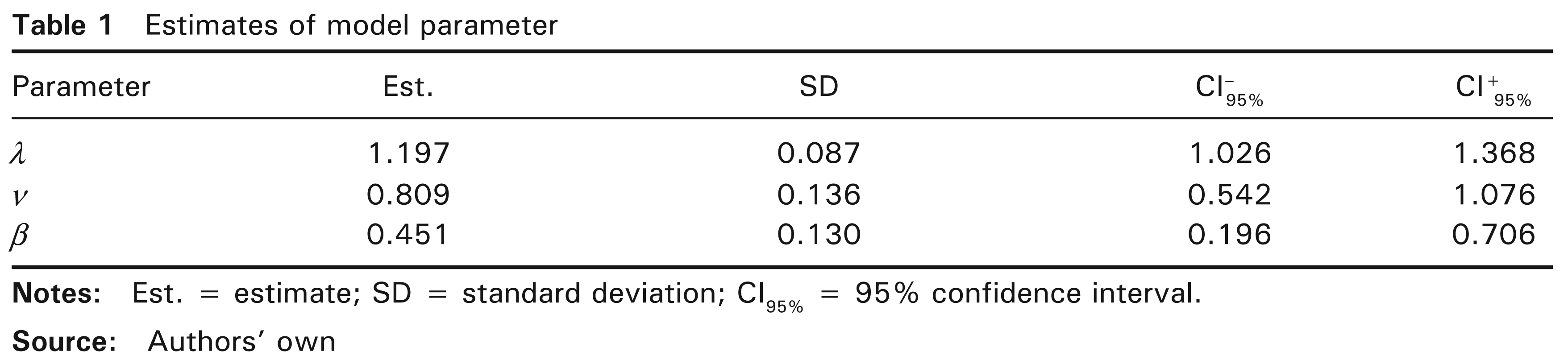
To solve the optimization problem and thereby find the MLE (see Section 3), we used the following two R software packages consecutively: DEoptim (Ardia et al., 2011) to find starting values, and alabama (Varadhan, 2011) to implement constrained optimization. The optimization algorithm was applied to a sample made up of full range of initial values to ensure that the global maximum is obtained. Through the differential evolution algorithm, DEoptim performs global optimization (for more details, see Mullen et al., 2011). In the alabama package, the constrOptim.nl and auglag functions use the augmented Lagrangian and adaptive barrier minimization algorithm in which constraints are allowed. Note that an approximate Hessian matrix can be provided both by the auglag function and by the fdHess function in the nlme R package using finite differences (Pinheiro et al., 2010). By considering the model without covariates, estimates of the three parameters and associated standard deviations and confidence intervals are obtained as set out in Table 1. Note that the model was globally significant because estimates were relatively accurate (with narrow CI). In addition, the estimator $\hat{β}$ was significantly different from zero according to the Wald test (W = 3.47, P-value = 0.0005) which confirmed the existence of the link between PFS and PPS thus consolidating the conditional model. As $\hat{β}$ was also positive, it means there was a positive correlation between PFS and PPS as well as between PFS and OS. Estimates of correlations with their standard deviations and confidence intervals are set out in Table 2. Correlation between PPS and PFS was relatively moderate while between PFS and OS it was very good. In other words, improvement in PFS was strongly associated with improvement in OS. The estimated PFS, PPS and OS curves using the proposed model are plotted in Figure 2 versus the nonparametric Kaplan–Meier estimator curve. Using the proposed model the median OS in years was 1.14, the median PFS 0.57 and the median PPS 0.44. Since there is a close fit between the empirical and the proposed model curves, the proposed model provides a reasonable estimate of OS as well as PFS and PPS.

5.3 Covariates

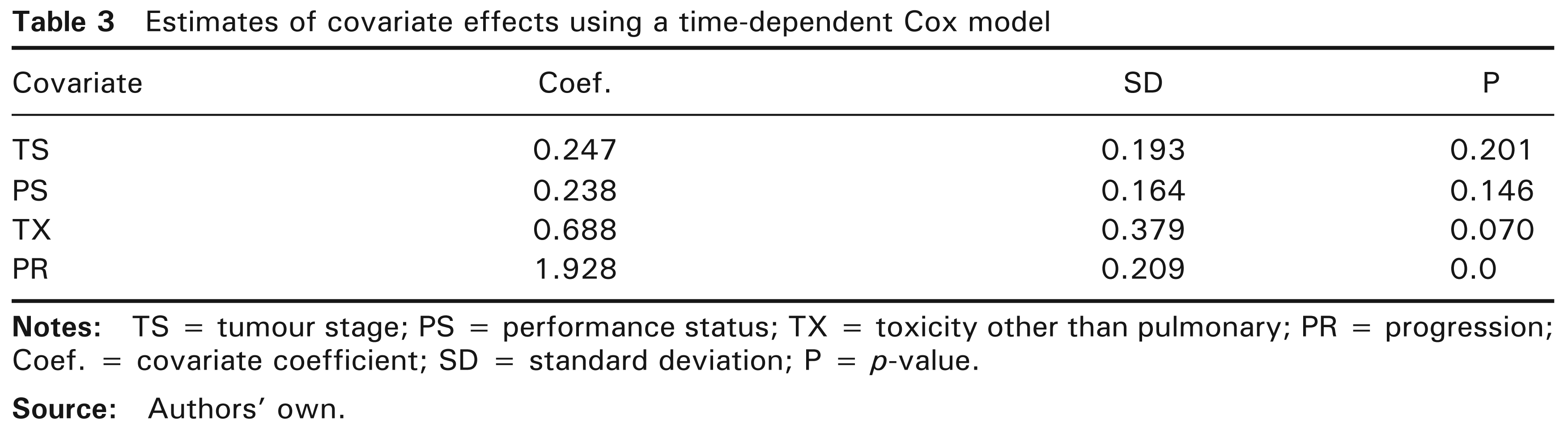
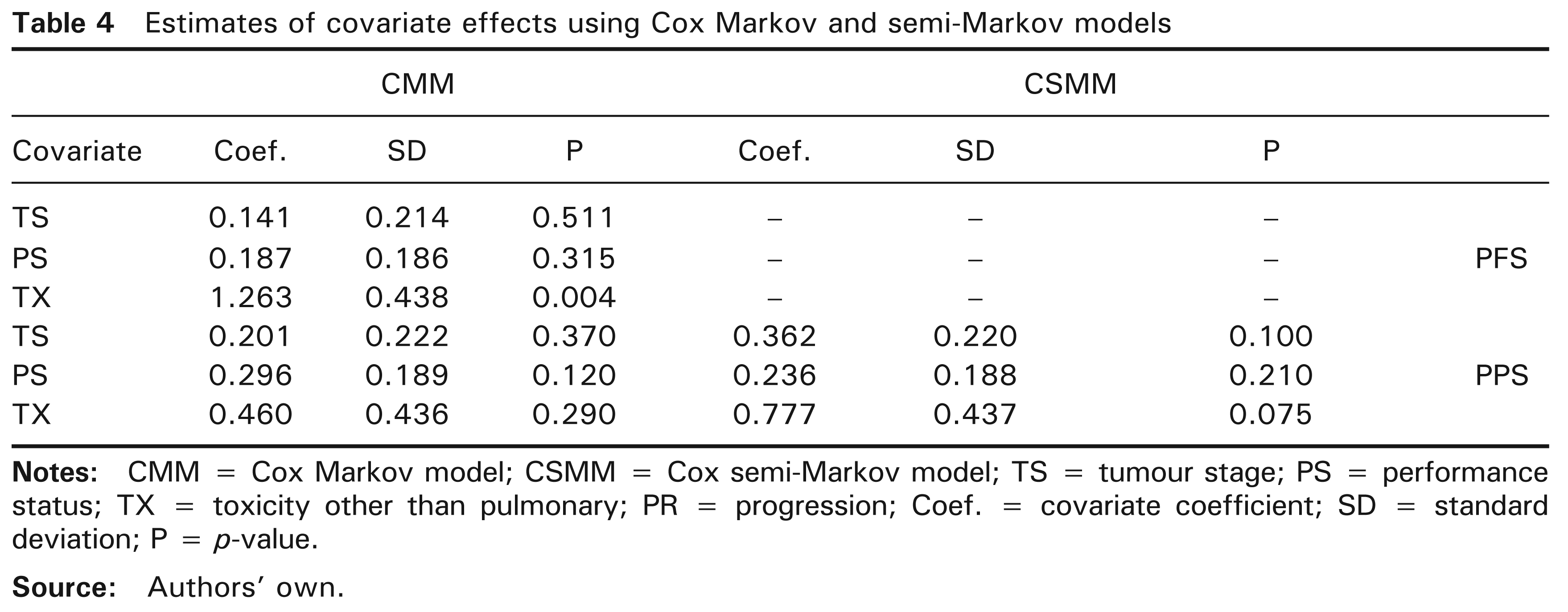
Moreover, for each patient, the database contains other available information than survival times. We used the nonparametric log-rank and generalized Wilcoxon tests with a threshold of 15% (not shown) in order to retain only the relevant covariates. The included covariates were: tumour stage (TS) coded as [0 = 3A stage; 1 = 3B stage], performance status (PS) coded as [0 = capable of normal activity; 1 = otherwise] and toxicity other than pulmonary (TX) coded as [0 = grade 0-1-2; 1 = grade 3–4]. While TX has a potential effect on PFS, PPS and OS, TS and PS have a potential effect on PPS and OS. The proportionality assumption is verified and there are globally 11 missing values in this set of covariates. However, since the purpose is to illustrate the introduction of covariates to the proposed model, the missing values were removed. Also, let progression (PR) be the time-dependent covariate coded as [0 = no tumour progression; 1 = tumour progression]. We first constructed a time-dependent Cox model (TDCM) including PR, among the three other covariates and Table 3 shows the estimates with their standard deviations and Wald P-values. Progressor patients had higher mortality than non-progressor patients. A significant effect of PR on mortality was fully expected. By taking 10% as threshold instead of the 5% default value, TX also affected mortality. The covariates TS and PS turned out to be insignificantly different from zero. In addition, the multi-state models represent an alternative to TDCM and offer further information. With a three-state model, it is even more interesting to study the covariate effects on PFS and PPS or in other terms the risk of progression and the risk of mortality after tumour progression. For such models, the Markov property is only relevant for the transition from tumour progression state to death state. However, the significance of $\hat{β}$ rejects this property by confirming that the transition intensity of mortality after tumour progression is affected by the time spent in the free-progression state. This means that a semi-Markov model is likely to be more appropriate for such a transition than a Markov model. The transition intensities may be modelled using Cox-like models; a Cox Markov model (CMM) for the progression intensity and a Cox semi-Markov model (CSMM) for the mortality intensity after the occurrence of the progression (for more details, see Andersen et al., 2000; Meira-Machado et al., 2009). Note that CMM without covariates is a time-inhomogeneous nonparametric model. In addition, we have re-estimated the proposed model parameters including covariate coefficients (as seen in Section 4). The only difference between CMM and CSMM concerns PPS. The estimated CMM and CSMM coefficients are shown in Table 4 and the estimated parameters using the proposed model are shown in Table 5. TX identified in TDCM turned out to affect PFS very significantly. Toxicity other than pulmonary seems to increase progression intensity. Regarding TX effect on PFS, estimates of CMM/CSMM and the proposed model are in agreement. TS and PS have no impact on PPS. Unlike CMM, the proposed model shows that TX also had a positive effect on PPS as does CSMM when taking 10% as threshold. Furthermore, as shown in Figure 3, there is a very close match between the TDCM and the proposed model survival curves. However, the proposed model seemed to be a better estimate for OS than CSMM especially regarding the tail of the survival curve.

Table 1

Estimates of model parameter

Parameter	Est.	SD	CI^–_95%	CI⁺_95%
λ	1.197	0.087	1.026	1.368
ν	0.809	0.136	0.542	1.076
β	0.451	0.130	0.196	0.706

Notes: Est. = estimate; SD = standard deviation; CI_95% = 95% confidence interval.

Source: Authors’ own

Table 2

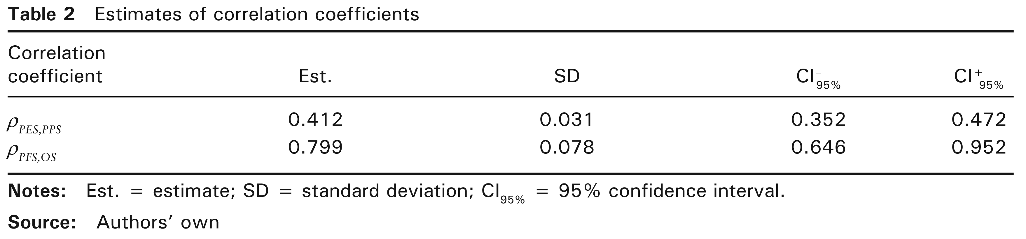
of correlation coefficients

Correlation coefficient	Est.	SD	CI^–_95%	CI⁺_95%
ρ_PES,PPS	0.412	0.031	0.352	0.472
ρ_PFS,OS	0.799	0.078	0.646	0.952

Notes: Est. = estimate; SD = standard deviation; CI_95% = 95% confidence interval.

Source: Authors’ own

Figure 2

Source: Authors’ own.

Table 3

Estimates of covariate effects using a time-dependent Cox model

Covariate	Coef.	SD	P
TS	0.247	0.193	0.201
PS	0.238	0.164	0.146
TX	0.688	0.379	0.070
PR	1.928	0.209	0.0

Notes: TS = tumour stage; PS = performance status; TX = toxicity other than pulmonary; PR = progression; Coef. = covariate coefficient; SD = standard deviation; P = p-value.

Source: Authors’ own.

Table 4

Estimates of covariate effects using Cox Markov and semi-Markov models

CMM				CSMM
Covariate	Coef.	SD	P	Coef.	SD	P
TS	0.141	0.214	0.511	–	–	–
PS	0.187	0.186	0.315	–	–	–	PFS
TX	1.263	0.438	0.004	–	–	–
TS	0.201	0.222	0.370	0.362	0.220	0.100
PS	0.296	0.189	0.120	0.236	0.188	0.210	PPS
TX	0.460	0.436	0.290	0.777	0.437	0.075

Notes: CMM = Cox Markov model; CSMM = Cox semi-Markov model; TS = tumour stage; PS = performance status; TX = toxicity other than pulmonary; PR = progression; Coef. = covariate coefficient; SD = standard deviation; P = p-value.

Source: Authors’ own.

Table 5

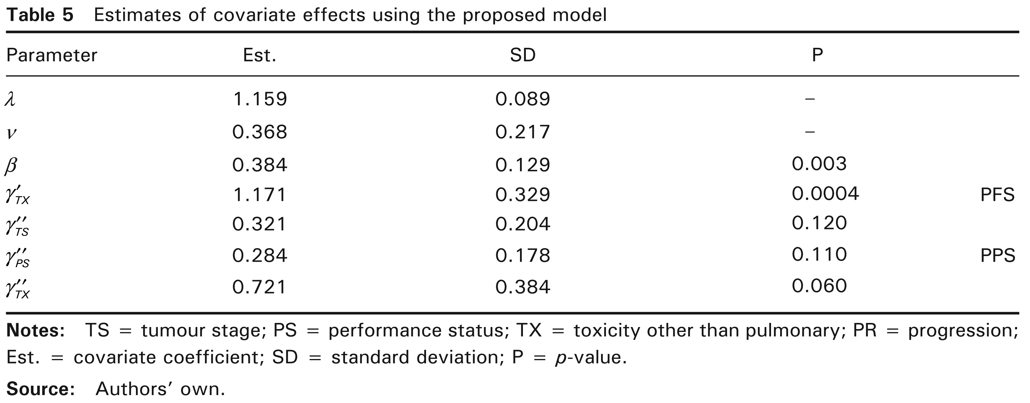
Estimates of covariate effects using the proposed model

Parameter	Est.	SD	P
λ	1.159	0.089	–
ν	0.368	0.217	–
β	0.384	0.129	0.003
${γ^{'}}_{T X}$	1.171	0.329	0.0004	PFS
${γ^{'}}^{'}_{T S}$	0.321	0.204	0.120
${γ^{'}}^{'}_{P S}$	0.284	0.178	0.110	PPS
${γ^{'}}^{'}_{T X}$	0.721	0.384	0.060

Notes: TS = tumour stage; PS = performance status; TX = toxicity other than pulmonary; PR = progression; Est. = covariate coefficient; SD = standard deviation; P = p-value.

Source: Authors’ own.

Figure 3

Source: Authors’ own.

6 Discussion

In oncology drugs clinical trials, OS is considered as the gold standard primary endpoint of clinical efficacy. Moreover and for obvious reasons (see Section 1), PFS may potentially replace and predict OS. According to US FDA (2007), OS is defined as the time from randomization until death from any cause and PFS as the time elapsed between randomization and tumour progression or death from any cause, too. It must be emphasized that cause of death information (patient status) may be missing for patients lost to follow-up or unknown for patients whose cause of death is dificult to determine as long as there is no evidence of disease neither in the last medical visit nor in autopsy (Andersen et al., 1996). In this instance, the use of multiple imputation methods (see Lu and Tsiatis, 2001; Nicolaie et al., 2011) is the best way to overcome this problem.

A parametric modelling of OS has been developed in this article. In order to understand the relationship between PFS and OS, we have considered OS as two consecutive survival times which are assumed to be dependent, PFS and PPS. This assumption is represented by conditional distribution, a link between PFS and PPS. In the proposed model, we considered a particular combination of exponential distributions both for PFS and for PPS|PFS. The primary advantage of exponential distribution is that the analysis is much simpler mathematically. With that combination, it should be noted that the generalization of the exponential distribution for PFS via Weibull distribution is numerically feasible. However, the calculation of correlations and estimates of moments are not analytically possible.

Prentice (1989) criteria are designed to validate surrogate endpoints in Phase III clinical trials. These criteria foremost require that the surrogate must be a correlate of the true clinical endpoint. Correlation is a necessary condition to confirm the possibility that the surrogate may predict the true endpoint, but it is not sufficient to conclude that the surrogate can replace the clinical endpoint. A correlation indicator (β) and formulas for the correlations between PFS and both PPS and OS were demonstrated. Generally, if PFS and OS are positively correlated, improvement in PFS is likely to lead to improvement in OS. However, in this case, deducing that PFS is positively correlated with PPS is not always true because it is possible that the lengthening of PFS will offset the decrement in PPS and thus the correlation between PFS and PPS will be negative. By finding significant positive correlations between PFS and OS, several studies have proposed PFS as the most appropriate surrogate endpoint for OS, most notably Buyse et al. (2007) who used individual patient data from several historical trials in advanced colorectal cancer, also Louvet et al. (2001) who handled 29 Phase III studies involving 13,498 patients and Tang et al. (2007) who analyzed 39 randomized trials including 87 treatment arms in metastatic colorectal cancer. In extensive stage small-cell lung cancer (SCLC), Foster et al. (2011) exploited individual patient data regrouping 596 patients from 3 randomized trials and 870 untreated patients to investigate the association of PFS with OS. By showing a strong correlation, they also considered PFS as a promising substitute for OS in extensive stage SCLC, but for validation, it would be necessary to use more data from randomized Phase III trials.

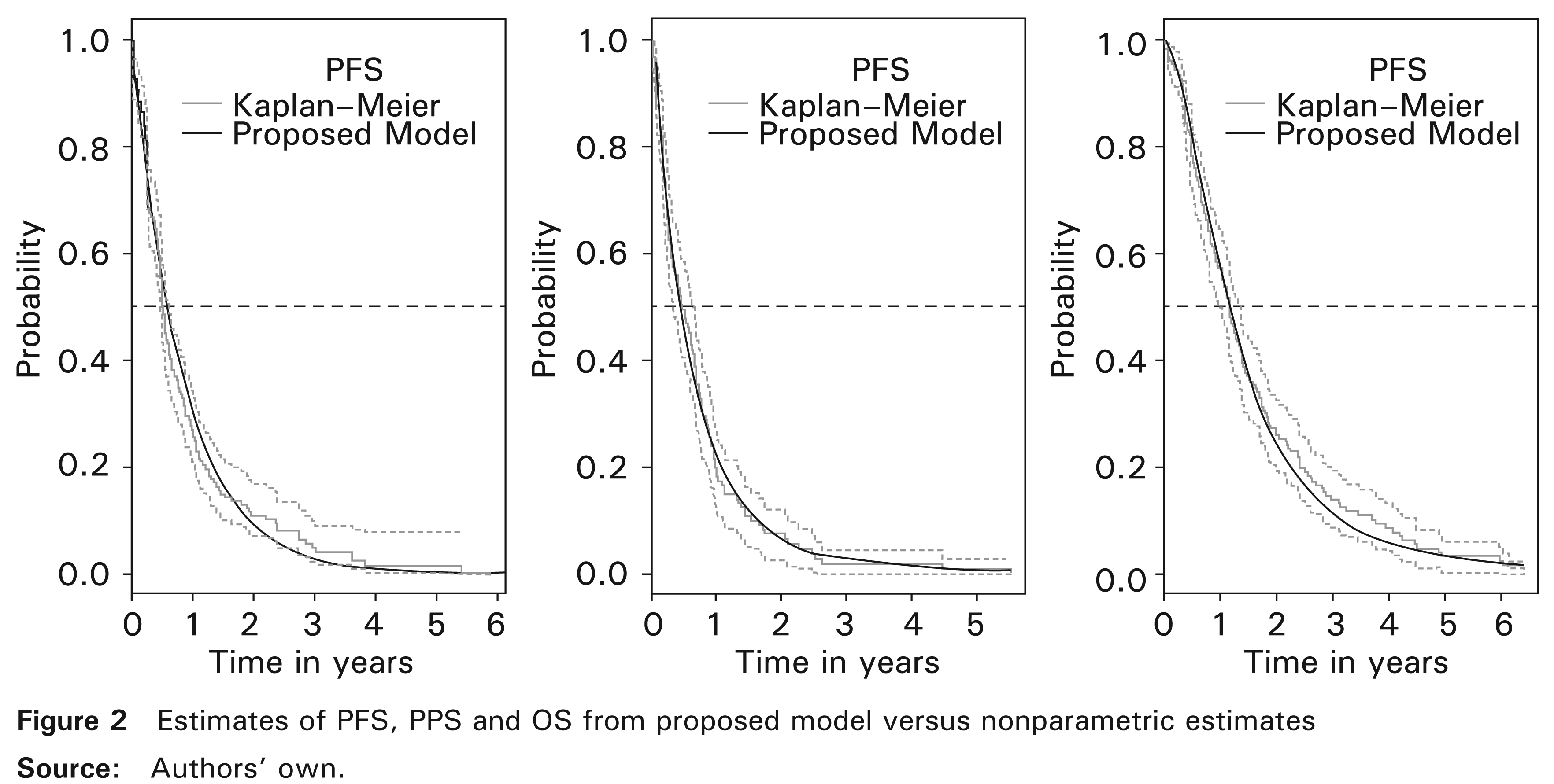
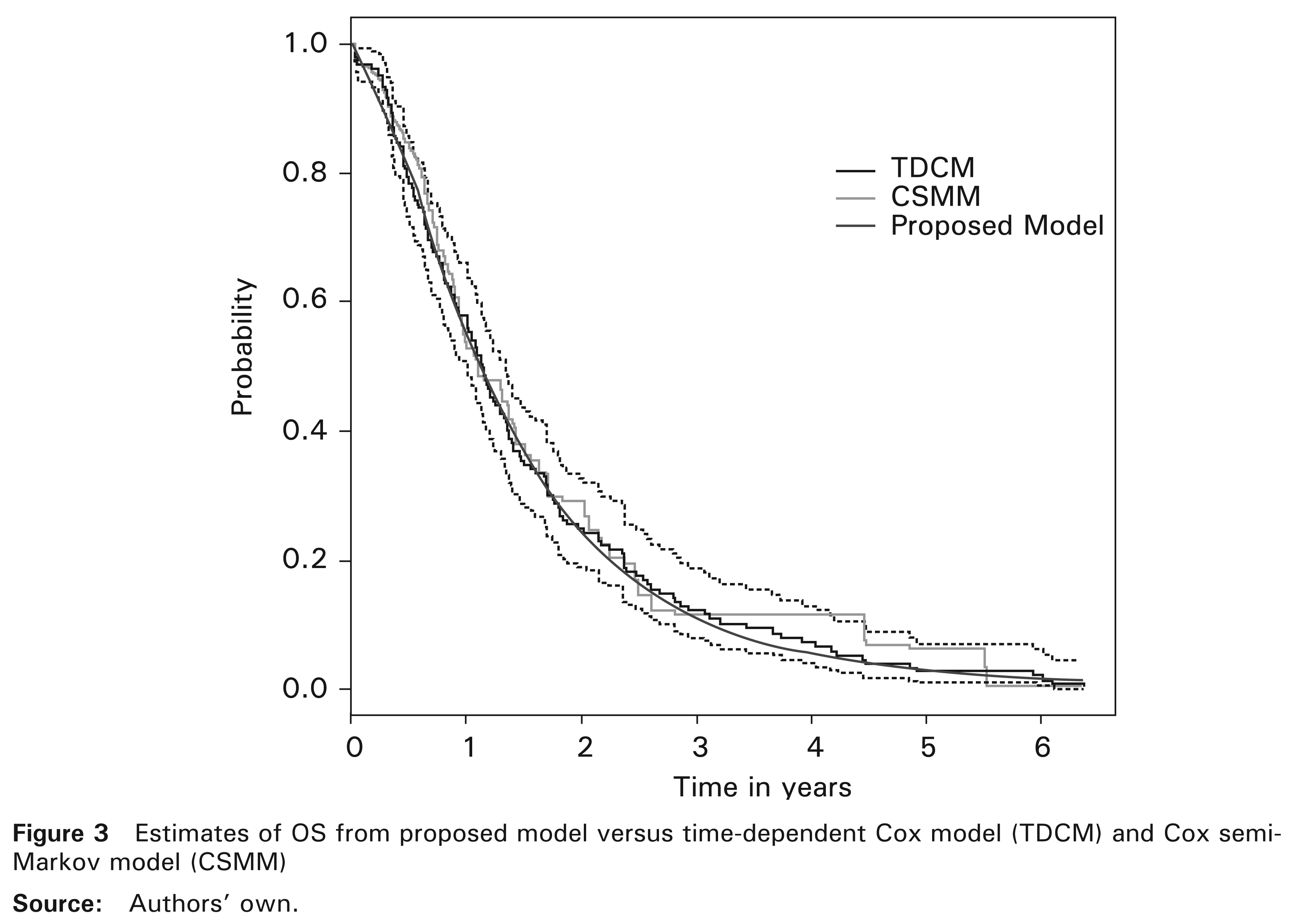
The model introduced here allows for the prediction of dependencies between PFS and PPS as well as between PFS and OS. We have applied it to randomized Phase III data with patients suffering from locally advanced NSCLC (Fournel et al., 2005). Note that in this database, Weibull distribution for PFS was reduced significantly to an exponential distribution which consolidated the choice of the latter. The numerical results were consistent with those reported by the cited authors and in agreement with those obtained by Fleischer et al. (2009) concerning the same disease. However, their model was built differently and it did not take into account the dependence between PFS and PPS. With no information about subsequent therapies in this database, we found a significantly positive correlation indicator (β > 0) proving the existence of a positive association between PFS and PPS and also between PFS and OS. This means most probably that improvement in PFS has led to the lengthening of PPS and consequently to improvement in OS. Second-line treatment is usually an optimal medical therapy since it is selected based on tumour type and clinical guidelines. For instance, the clinical practice guideline proposed by Noble et al. (2006) for recurrent or progressive NSCLC. Otherwise, the proposed model can take into account the effect of subsequent therapies on mortality. Indeed, the form of the proposed model allows for multiple covariates including first-line treatment, baseline covariates and subsequent therapies. In addition, the proposed model and CSMM (Andersen et al., 2000; Meira-Machado et al., 2009) seemed to have the same ability to detect significant effects of covariates. Also, the survival probability estimates based on the proposed model seemed to closely match the nonparametric Kaplan–Meier estimator and TDCM.

In fact, with the strong positive correlation found between PFS and OS, PFS seems to be a good potential surrogate for OS in locally advanced NSCLC trials. However, parameter estimates require the use of data from large carefully selected samples. The question raised is whether PFS will be valid as a surrogate for OS with all the treatments used for the disease concerned. One can possibly answer this question by conducting a meta-analysis which includes these treatments with individual patient data using our modelling. This procedure was previously exploited by Buyse et al. (2007) for colorectal cancer treatments. In conclusion, the proposed model generalizes the structure of dependency between PFS and OS and allows for better understanding of the process of OS improvement or decrement by means of PFS and PPS. It also provides a flexible tool for survival probability estimation and the study of covariate effects.

Footnotes

Acknowledgements

Mohamed C. Belkacemi is the recipient of a fellowship from the Algerian Ministry of Higher Education and Scientific Research.

Appendix

We found the following results, given that

X ∼ Exp(λ), then E(X) = 1/λand Var(X) = 1/λ².

Y|X ∼ Exp(θ_Y_|X(x)) and θ_Y_|X(x) = αexp(–β(x) where α = exp(ν) and β < λ/2, then E(Y | X) = 1/θ_Y_|X(x) and Var(Y | X) = 1/θ_Y_|X(x)².

We calculated the first moment of Y and thus that of T

= \frac{λ}{α} \int_{0}^{\infty} \exp {- (λ - β) x} d x

= \frac{λ}{α (λ - β)}

and

E (T) = E (X) + E (Y) = \frac{λ^{2} + α (λ - β)}{α λ (λ - β)} .

In addition, the covariance between X and Y was obtained by

Cov (X, Y) = E (X Y) - E (X) E (Y),

where

E (X Y) = \int_{0}^{\infty} \int_{0}^{\infty} x y f_{X, Y} (x, y) d x d y

= \int_{0}^{\infty} E (Y | X) x f_{X} (x) d x

= \frac{λ}{α} \int_{0}^{\infty} x \exp {- (λ - β) x} d x

= \frac{λ}{α {(λ - β)}^{2}}

and therefore,

Cov (X, Y) = \frac{λ}{α {(λ - β)}^{2}} - \frac{λ}{α (λ - β) λ}

= \frac{β}{α {(λ - β)}^{2}} .

Using this result, we found the covariance between T and X

= \frac{(α + β) λ^{2} - 2 α β λ + α β^{2}}{α λ^{2} {(λ - β)}^{2}} .

We also calculated the second moment of Y

= \int_{0}^{\infty} \frac{2 e x p (2 β x)}{α^{2}} λ exp (- λ x) d x

= \frac{2 λ}{α^{2}} \int_{0}^{\infty} \exp {- (λ - 2 β) x} d x

= \frac{2 λ}{α^{2} (λ - 2 β)}

Therefore,

Var (Y) = \frac{λ {{(λ - β)}^{2} + β^{2}}}{α^{2} {(λ - β)}^{2} (λ - 2 β)}

and

= \frac{1}{λ^{2}} + \frac{λ {{(λ - β)}^{2} + β^{2}} + 2 α β (λ - 2 β)}{α^{2} {(λ - β)}^{2} (λ - 2 β)} .

Furthermore, given that the correlation coefficient between X and Y is equal to

Corr (X, Y) = \frac{Cov (X, Y)}{\sqrt{Var (X) Var (Y)}},

we finally found the correlation coefficients

Corr (X, Y) = \frac{β}{λ - β} \sqrt{\frac{λ (λ - 2 β)}{{(λ - β)}^{2} + β^{2}}}

and also

Corr (X, T) = \frac{(α + β) λ^{2} - α β (2 λ - β)}{α λ {(λ - β)}^{2} \sqrt{Var (T)}} .

Moreover, by combining regularity conditions with the Lindeberg-Feller central limit theorem, the MLE vector

\hat{Ψ} = (\begin{matrix} \hat{λ} \\ \hat{ν} \\ \hat{β} \end{matrix})

asymptotically satisfies

\hat{Ψ} \overset{d}{\to} N (Ψ, I_{\hat{Ψ}}^{- 1}),

where $I_{\hat{Ψ}}$ is the Fisher information matrix of second-order partial derivatives (Hessian matrix) of the log-likelihood with respect to the three parameters. Then, this leads to

Φ (\hat{Ψ}) \overset{d}{\to} N (Φ (Ψ), Var {Φ (\hat{Ψ})}),

Var {Φ (\hat{Ψ})} \approx \frac{δ Φ (Ψ)}{δ Ψ^{'}} |_{Ψ = \hat{Ψ}} Σ_{\hat{Ψ}} \frac{δ Φ (Ψ)}{δ Ψ} |_{Ψ = \hat{Ψ}},

where $\frac{δ Φ (Ψ)}{δ Ψ}$ is the vector of the first partial derivatives and the asymptotic variance–covariance matrix $Σ_{\hat{Ψ}} = I_{\hat{Ψ}}^{- 1} .$

References

Aalen Odd

Johansen

Søren

(1978) An empirical transition matrix for non-homogeneous Markov chains based on censored observations. Scandinavian Journal of Statistics, 5, 141–50.

Andersen

Goetghebeur

Ryan

(1996) Missing cause of death information in the analysis of survival data. Statistics in Medicine, 15, 2191–201.

Andersen

Per Kragh

Keiding

Niels

(2002) Multi-state models for event history analysis. Statistical Methods in Medical Research, 11, 91–115.

Andersen

Per Kragh

Esbjerg

Sille

Sørensen Thorkild

(2000) Multi-state models for bleeding episodes and mortality in liver cirrhosis. Statistics in Medicine, 19, 587–99.

Ardia

Mullen

Peterson

Ulrich

Mullen

(2011) Deoptim: global optimization by differential evolution. http://cran.r-project.org/web/packages/DEoptim/.

Ballman

Buckner

Brown

Giannini

Flynn

LaPlant

Jaeckle

(2007) The relationship between six-month progression-free survival and 12-month overall survival end points for phase II trials in patients with glioblastoma multiforme. Neuro-Oncology, 9, 29.

Begg

Larson

(1982) A study of the use of the probability-of-being-in-response function as a summary of tumour response data. Biometrics, 38(1), 59–66.

Burzykowski

Buyse

Piccart-Gebhart

Sledge

Carmichael

Lück

Mackey

Nabholtz

Paridaens

Biganzoli

. (2008) Evaluation of tumour response, disease control, progression-free survival, and time to progression as potential surrogate end points in metastatic breast cancer. Journal of Clinical Oncology, 26, 1987–92.

Buyse

Burzykowski

Carroll

Michiels

Sargent

Miller

Elfring

Pignon

Piedbois

(2007) Progression-free survival is a surrogate for survival in advanced colorectal cancer. Journal of Clinical Oncology, 25, 5218.

10.

Cox David

(1972) Regression models and life-tables. Journal of the Royal Statistical Society. Series B (Methodological), 34(2), 187–220.

11.

Cox

Miller

(1965) The theory of stochastic processes. London: Methuen.

12.

Datta

Somnath

Satten Glen

(2001) Validity of the Aalen–Johansen estimators of stage occupation probabilities and Nelson–Aalen estimators of integrated transition hazards for non-Markov models. Statistics & Probability letters, 55, 403–11.

13.

Eisenhauer

Therasse

Bogaerts

Schwartz

Sargent

Ford

Dancey

Arbuck

Gwyther

Mooney

. (2009) New response evaluation criteria in solid tumours: revised RECIST guideline (version 1.1). European Journal of Cancer, 45, 228–47.

14.

Ellis

Carroll

Pemberton

(2008) Analysis of duration of response in oncology trials. Contemporary Clinical Trials, 29, 456–65.

15.

Fleischer

Gaschler-Markefski

Bluhmki

(2009) A statistical model for the dependence between progression-free survival and overall survival. Statistics in Medicine, 28, 2669–86.

16.

Foster

Shi

Krook

Kugler

Jett

Molina

Schild

Adjei

Mandrekar

(2011) Tumour response and progression-free survival as potential surrogate endpoints for overall survival in extensive stage small-cell lung cancer. Cancer, 117(6), 1262–1271.

17.

Fournel

Robinet

Thomas

Souquet

Lêna

Vergnenégre

Delhoume

Le Treut

Silvani

Dansin

. (2005) Randomized phase III trial of sequential chemoradiotherapy compared with concurrent chemoradiotherapy in locally advanced non-small-cell lung cancer: Groupe Lyon-Saint-Etienne d’Oncologie Thoracique – Groupe Francais de Pneumo-Cancérologie NPC 95-01 study. Journal of Clinical Oncology, 23, 5910–17.

18.

Greene William

Zhang

Chengsi

(1997) Econometric analysis, volume 3. Upper Saddle River, NJ: Prentice Hall.

19.

Heng

DYC

Xie

Bjarnason

Vaishampayan

Tan

Knox

Donskov

Wood

Kollmannsberger

Rini

. (2011) Progression-free survival as a predictor of overall survival in metastatic renal cell carcinoma treated with contemporary targeted therapy. Cancer, 117(12), 2367–2642.

20.

Hurvitz

(2011) Evolving options for the treatment of metastatic breast cancer: progression-free survival as an endpoint. Cancer Treatment Reviews, 37(7), 495–504.

21.

Kaplan

Meier

(1958) Nonparametric estimation from incomplete observations. Journal of the American Statistical Association, 53(282), 457–81.

22.

Komaki

Scoot

Lee

Fossella

Dundas

McDonald

Palmer

Curran

Byhardt

. (1994) Phase I/II study of combined chemoradiation with cisplatin plus oral etoposide for patients with locally advanced inoperable non-small-cell lung cancer: RTOG 91–06. Lung Cancer, 11 (suppl. 1), 178 (A690).

23.

Lamborn

Yung

Chang

Wen

Cloughesy

DeAngelis

Robins

Lieberman

Fine

Fink

. (2008) Progression-free survival: an important end point in evaluating therapy for recurrent high-grade gliomas. Neuro-Oncology, 10, 162.

24.

Le Chevalier

Brisgand

Douillard

Pujol

Alberola

Monnier

Riviere

Lianes

Chomy

Cigolari

(1994) Randomized study of vinorelbine and cisplatin versus vindesine and cisplatin versus vinorelbine alone in advanced non-small-cell lung cancer: results of a European multicenter trial including 612 patients. Journal of Clinical Oncology, 12, 360.

25.

Lee

Scott

Komaki

Fossella

Dundas

McDonald

Byhardt

Curran

(1996) Concurrent chemoradiation therapy with oral etoposide and cisplatin for locally advanced inoperable non-small-cell lung cancer: radiation therapy oncology group protocol 91–06. Journal of Clinical Oncology, 14, 1055.

26.

Louvet

de Gramont

Tournigand

Artru

Maindrault-Goebel

Krulik

(2001) Correlation between progression free survival and response rate in patients with metastatic colorectal carcinoma. Cancer, 91, 2033–38.

27.

Tsiatis

(2001) Multiple imputation methods for estimating regression coeffi¬cients in the competing risks model with missing cause of failure. Biometrics, 57, 1191–97.

28.

Mayfield

(2008) Progression-free survival: patient benefit or lower standard? NCI Cancer Bulletin, 5, 8–9.

29.

Meira-Machado

Luis

De Una-Alvarez

Jacobo

Cadarso-Suarez

Carmen

(2006) Nonparametric estimation of transition probabilities in a non-Markov illness–death model. Lifetime Data Analysis, 12, 325–44.

30.

Meira-Machado

Lus

de Uña-Álvarez

Jacobo

Cadarso-Suarez

Carmen

Andersen Per

(2009) Multi-state models for the analysis of time-to-event data. Statistical Methods in Medical Research, 18, 195–222.

31.

Mullen

Ardia

Gil

Windover

Cline

(2011) Deoptim: an R package for global optimization by differential evolution. Journal of Statistical Software, 40, 1–26.

32.

Nicolaie

van Houwelingen

Putter

(2011) Vertical modeling: analysis of competing risks data with missing causes of failure. Statistical Methods in Medical Research. Epub ahead of print. doi: 10.1177/0962280211432067.

33.

Noble

Ellis

Mackay

Evans

and Lung Cancer Disease Site Group of Cancer Care Ontario’s Program in Evidence-based Care (2006) Second-line or subsequent systemic therapy for recurrent or progressive non-small cell lung cancer: a systematic review and practice guideline. Journal of Thoracic Oncology, 1, 1042–58.

34.

Pepe Margaret

Sullivan

(1991) Inference for events with dependent risks in multiple endpoint studies. Journal of the American Statistical Association, 86, 770–78.

35.

Perez-Ocon

Rafael

Eloy

Ruiz-Castro Juan

Luz

Gamiz-Perez M

(2001) A piecewise Markov process for analysing survival from breast cancer in different risk groups. Statistics in Medicine, 20, 109–22.

36.

Pinheiro

Bates

DebRoy

Sarkar

(2010) nlme: linear and nonlinear mixed effects models. http://cran.r-project.org/web/packages/nlme/.

37.

Porzsolt

Weber

Muche

(2009) 28LBA conceptual change in oncology: progression-free-survival is a more appropriate surrogate for overall survival than time-to-progression. EJC Supplements, 7, 15–15.

38.

Prentice Ross

(1989) Surrogate endpoints in clinical trials: definition and operational criteria. Statistics in Medicine, 8, 431–40.

39.

Singh

Law

(2010) Utility of progression-free survival as a primary endpoint in clinical studies of advanced neuroendocrine tumours. Annals of Oncology. The 35th European Society for Medical Oncology Congress. Neuroendocrine tumours and CUP. 851P, 21.

40.

Saad

Katz

Hoff

Buyse

(2010) Progression-free survival as surrogate and as true end point: insights from the breast and colorectal cancer literature. Annals of Oncology, 21, 7–12.

41.

Sherrill

Hirst

Amonkar

Stein

(2007) Correlation between time to progression and overall survival in patients with metastatic breast cancer. In: ISPOR, 12th Annual International Meeting of the International Society for Pharmacoeconomics and Outcomes Research 19–23 May 2007, Arlington, VA, USA.

42.

Strauss

David

Shavelle

Robert

(1998) An extended Kaplan–Meier estimator and its applications. Statistics in Medicine, 17, 971–82.

43.

Tang

Bentzen

Chen

Siu

(2007) Surrogate end points for median overall survival in metastatic colorectal cancer: literature-based analysis from 39 randomized controlled trials of first-line chemotherapy. Journal of Clinical Oncology, 25, 4562.

44.

Therasse

Arbuck

Eisenhauer

Wanders

Kaplan

Rubinstein

Verweij

Van Glabbeke

Van Oosterom

Christian

, . (2000) New guidelines to evaluate the response to treatment in solid tumours. Journal of the National Cancer Institute, 92, 205.

45.

FDA US (2007) Drug administration guidance for industry: clinical trial endpoints for the approval of cancer drugs and biologics. Washington, DC: US Food and Drug Administration, pp. 1–19.

46.

Varadhan

(2011) alabama: constrained nonlinear optimization. With contributions from Grothendieck, G. http://cran.r-project.org/web/packages/alabama/.

47.

Yuan

Thall

Wolff

(2011) Estimating progression-free survival in paediatric brain tumour patients when some progression statuses are unknown. Journal of the Royal Statistical Society: Series C (Applied Statistics), 61(1), 135–49.