Non-parametric regression for compositional data

Abstract

Regression for compositional data has been considered only from a parametric point of view. We introduce local constant and local linear smoothing for this problem, and treat the cases when the response, the predictor or both of them are compositions. To this end, we introduce suitable series expansions of the regression function at a point, along with a class of simplicial kernels. Our methods are formulated according to the Aitchison geometry of the simplex and then, using some relevant properties of the isometric log-ratio transformation, are developed following the principle of ‘working on coordinates’. Asymptotic properties and real-data case studies show the effectiveness of the methods.

Keywords

isometric log-ratio (ilr) transformation local constant fit local linear fit simplicial kernels soil composition

1 Introduction

Compositional data, or compositions, are sets of portions of a whole. A D-part composition, D ₊, lies on the simplex

^{D} : \{(x_{1},, x_{D})^{} : x_{i} > 0, i 1,, D;_{i 1}^{D} x_{i} k\},

where k is a positive real constant.

Typical examples of compositional data include mineral compositions of rocks, proportions of pollutants in air or in rivers, compositions of electorates, distributions of financial funds or percentages of expenditures in a country. For a recent comprehensive account on compositional data see Pawlowsky-Glahn and Buccianti (2011) and the references therein.

A simple approach to statistical analysis of compositional data uses transformations into the Euclidean space. Egozcue et al. (2003) introduced the isometric log-ratio (ilr) transformation of D-parts compositions. Such transformation gives coordinates in ^D–1 (ilr coordinates), and exhibits some advantages with respect to the previously proposed transformations.

The case of a real-valued response predicted by a composition has been traditionally modelled using various polynomial forms of the parts of the predictor by Scheffè (1958) and Scheffè (1963). Additionally, Aitchison and Bacon-Shone (1984) proposed to work with log transformations of the predictors, which, clearly, removes the constraint of a constant sum. Recently, Hron et al. (2012) discussed a linear model based on ilr coordinates representation, overcoming some interpretability drawbacks arising from the previous models, and allowing standard inference on the parameters.

Aitchison (1982) and Hijazi and Jernigan (2009) modelled regression of a compositional response on a real predictor assuming, as distribution for residuals, the Dirichlet or the logistic-normal distributions. For the same problem, Tolosana-Delgado and Van Den Boogart (2011) and Egozcue et al. (2012) proposed a linear model using ilr coordinates of the response, allowing ordinary least-squares theory on the space of coordinates. The above-mentioned approaches have a parametric nature.

Latterly, some work adapted non-parametric regression to non-Euclidean manifolds. For example, Di Marzio et al. (2013) pursue the circular case, and Di Marzio et al. (2014) the spherical one. The idea is to develop an intrinsic approach to get readily applicable methods without transforming data via link functions. Analogously, in the present paper, we introduce non-parametric estimators for the regression function when: i) the predictor is compositional and the response is real (simplicial-real regression); ii) the predictor and the response are both compositions (simplicial-simplicial regression); iii) the predictor is real and the response is compositional (real-simplicial regression). All of our smoothers have a local polynomial nature, where a derivative of the regression function is estimated as the coefficient of a term in the series expansion of the regression function at a point. Such a coefficient is found by solving a locally weighted least-squares problem. For each kind of regression, we discuss two estimators, the constant fit, which is based on a single-term expansion of the regression function, and the linear fit which, instead, uses two of such terms.

In Section 2, we collect some preliminaries on the Aitchison geometry of the simplex, along with some properties of the ilr transformation. Then, in Section 3, a class of simplicial kernels is introduced, and in Section 4 we consider non-parametric estimation of a simplicial-real regression function. Non-parametric estimation of the regression function with compositional response is the subject of Sections 5 and 6 for the cases where the predictor is compositional and real, respectively. In Section 7, we discuss directional smoothing for the simplicial response case. Finally, Section 8 provides some real-data applications, along with some comparisons with existing methods.

2 Preliminaries

Perturbation and powering are the basic operations in the Aitchison geometry (Aitchison, 1982, 1986). For D-part compositions x and y, and α ∈ , they are, respectively, defined as

x y : (x_{1} y_{1},, x_{D} y_{D})^{} and x : (x_{1}^{},, x_{D}^{})^{}

where $(u): (u_{1} /_{i 1}^{D} u_{i},, u_{D} /_{i 1}^{D} u_{i})^{}$ is the closure of $u_{}^{D}$ . Furthermore, the difference perturbation is defined as $x y : x ((1) y)$ .

Perturbation and powering induce a (D – 1)-dimensional real-vector space structure on ^D.

Let the set {e₁, …, e_D–1} be an orthonormal basis of ^D, and denote as U the associated basis-contrast matrix, i.e., the D (D – 1) matrix with ith column given by centred log-ratio (clr) clr(e_i), i ∈ {1, …, D – 1}, where for u ∈ ^D,

clr (u): {(\ln (u_{1} / \sqrt[D]{u_{1} u_{D}}),, \ln (u_{D} / \sqrt[D]{u_{1} u_{D}}))}^{}

The ilr transformation related to U, say ilr_U, is the one-to-one linear transformation relating the vector x* ∈ ^D–1 to x ∈ ^D, as follows:

x^{*} : {ilr}_{U} (x) U^{} clr (x) U^{} \ln (x)

The ilr transformation defines an isomorphism between ^D and ^D–1, i.e., for each x, y ∈ ^D and a ∈ ,

{ilr}_{U} (x y) {ilr}_{} (x) {ilr}_{U} (y), {ilr}_{} (x) {ilr}_{} (x)

and exhibits the property of being isometric, i.e., $d_{a} (x, y) {ilr}_{U} (x) {ilr}_{U} (y))$ , where

d_{a} (x, y): \sqrt{\frac{1}{D} \underset{i < j}{} {\{\ln (\frac{x_{i}}{x_{j}}) \ln (\frac{y_{i}}{y_{j}})\}}^{2}}

is the Aitchison distance, while stands for the Euclidean norm. Clearly, for x ∈ ^D, the Aitchison norm, which is defined as $x_{a} : d_{a} (x, n)$ , with n(1, …, 1)^{being the neutral element of perturbation, satisfies
$x_{a} {ilr}_{U} (x)$
. Note that zeros are not allowed in the definition of these metric elements. Those zero values need to be treated previously with specific techniques that can be found, e.g., in Martín-Fernandez et al. (2012) and references therein.}

Using Aitchison geometry, Pawlowsky-Glahn and Egozcue (2001) defined the centre and the metric variance of a D-part random composition X, respectively, as

Cen [X] : \underset{z}{argmin} E [d_{a}^{2} (X, z)] and Mvar [X]: E [d_{a}^{2} (X, Cen [X])]

which, using the ilr coordinates of X, can be respectively expressed as

Cen [X] {ilr}_{U}^{1} (E [{ilr}_{U} (X)]) and Mvar [X]_{i 1}^{D 1} Var [{ilr}_{U}^{(i)} (X)],

with ${ilr}_{U}^{(i)} (X)$ denoting the ith entry of ilr_U(X), i ∈ {1, ..., D – 1}.

From now on, we denote U and V as the basis-contrast matrices associated with selected orthonormal bases for ^D and ^L, respectively. Moreover, for a function g : ^D , let $\overset{}{g} :^{D 1}$ be the composite function $\overset{}{g} : g o {ilr}_{U}^{1}$ . Furthermore, for a function g : ^D ^L, we denote as g* : ^D–1 ^L–1 the function $g^{*} : {ilr}_{V} o g o {ilr}_{U}^{1}$ .

3 Kernels on the simplex

Kernels on the simplex have been introduced, for the task of density estimation, by Aitchison and Lauder (1985) and Chacón et al. (2011). First, the authors proposed the multivariate Dirichlet distribution, ‘recommended only when there is suspicion of sparseness in the data’, and the additive logistic normal kernel. The latter is based on a logarithmic transformation, and requires particular structures of the bandwidth matrix to guarantee the invariance of the estimate under permutation of the components. More recently, Chacón et al. (2011) introduced the isometric log-ratio normal kernel, which is based on the ilr transformation of data. Such kernel overcomes the drawbacks of the previous ones, having, in particular, the property of being invariant under changing of the orthonormal basis.

A class of simplicial kernels, which includes the isometric log-ratio normal kernel, can be constructed starting from univariate Euclidean ones as follows.

Definition 1. Let be a continuous function with maximum at 0 such that (–u)(u) ≥ 0, u ∈ , and $_{} (x) dx <$ . A D-variate simplicial kernel can be defined, for each u ∈ ^D, as

K (u): \frac{(u_{a})}{_{^{D}} (u_{a}) d_{a} (u)},

where $_{a}$ stands for the Aitchison measure on ^D.

Notice that i) for a set $A^{D}$ , $_{a} (A) ({ilr}_{U} (A))$ , with being the Lebesgue measure on ^D–1, and ii) $u_{a} u^{*}$ , for u*ilr_U(u). Therefore, a kernel in Definition 1 corresponds to a radially symmetric one in the space of coordinates, i.e.,

K (u) \overset{}{K} (u^{*}): \frac{(u^{*})}{_{^{D 1}} (u^{*}) d u^{*}} .

(3.1)

Notice that a simplicial kernel K in Definition 1 is a density on ^D with respect to the Aitchison measure, whereas $\overset{}{K}$ is a density on ^D–1 with respect to the Lebesgue measure.

Remark 1. It is easily seen that kernels in (3.1) are invariant under changing of orthonormal basis in ^D. In fact, letting ${ilr}_{U_{1}}$ and ${ilr}_{U_{2}}$ denote isometric log-ratio transformations corresponding to two different orthonormal bases, there exists an orthogonal matrix A such that ${ilr}_{U_{2}} (u) A {ilr}_{U_{1}} (u)$ , for each u ∈ ^D. Then, by orthogonality of A, it follows that ${ilr}_{U_{2}} (u) {ilr}_{U_{1}} (u)$ , and $d ({ilr}_{U_{2}} (u)) d ({ilr}_{U_{1}} (u))$ .

Using the same arguments as in Chacón et al. (2011), it can be easily seen that all kernels in this class match the property of being invariant under changing of basis for ^D. From (3.1), the order of a simplicial kernel can be defined as the order of the corresponding kernel in the space of coordinates. Specifically, letting be a second-order Euclidean kernel, the second moment of K is

M_{2} (K):_{^{D 1}} \overset{}{K} (u^{*}) u^{*} u^{*} d u^{*}_{2} (\overset{}{K}) I_{D 1},

(3.2)

with $_{2} (\overset{}{K}): {_{^{D 1}} u}_{i}^{* 2} \overset{}{K} (u^{}) d u^{*}$ , and I_s denoting the identity matrix of order $s_{}$ . Moreover, the following holds.

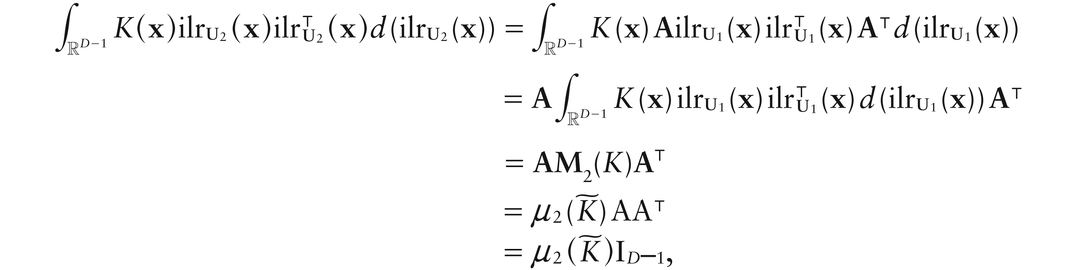
Result 1. Let K be a second-order simplicial kernel. Then, M₂(K) is unaffected by the choice of the basis for ^D.

Proof. See Appendix.

Let H be a symmetric positive definite matrix of order D – 1; then a simplicial kernel at x ∈ ^D, centered at y ∈ ^D and rescaled by H, is $K_{H} (x y) | H |^{1} \overset{}{K} (H^{1} (x^{*} y^{*}))$ .

Remark 2. It is easily seen that ${\overset{}{K}}_{H}$ is invariant under changing of orthonormal basis for ^D. In fact, letting ${ilr}_{U_{1}}$ and ${ilr}_{U_{2}}$ be the coordinates corresponding to two different orthonormal bases, and moreover, letting H⁽¹⁾ and H⁽²⁾ be the bandwidth matrices obtained using the respective ilr vectors, then there exists an orthogonal matrix A such that ${ilr}_{U_{2}} (x) A {ilr}_{U_{1}} (x)$ and $H^{(2)} A H^{(1)} A^{}$ . By orthogonality of A, it follows that $| H^{(2)} |^{1} | H^{(1)} |^{1}$ , and $H^{(2) 1} {ilr}_{U_{2}} () H^{(1) 1} {ilr}_{U_{1}} ()$ .

4 Simplicial-real regression

Given an ^D -valued random sample {(X_i, Y_i), i1, …, n}, assume the model

Y_{i} m (X_{i}) ɛ_{i},

where $m (x): E [Y | X x] <$ , and the ɛ_is, conditioned on the X_is, are independent and identically distributed real-valued random variables with E $[ɛ_{i} | X_{i}] 0$ and Var $[ɛ_{i} | X_{i}]^{2} (X_{i}) <$ . Then, a local constant estimator for m(x) can be defined as the solution of

\underset{b_{0}}{argmin}_{i 1}^{n} {Y_{i} b_{0}}^{2} K_{H} (X_{i} x),

with $K_{H} ()$ being a simplicial kernel in Definition 1, rescaled by the smoothing matrix H. This leads to

\overset{}{m} (x; H) \frac{_{i 1}^{n} K_{H} (X_{i} x) Y_{i}}{_{i 1}^{n} K_{H} (X_{i} x)} .

(4.1)

To obtain the local linear version of the above estimator, we recall the following.

Definition 2. A function $g :^{D}$ is called -differentiable at x ∈ ^D if there exists a unique 1 D vector D_g(x), satisfying D_g(x)1_D0, such that

\lim_{u \overset{}{} n} \frac{| g (x u) g (x)_{g} (x) \ln (u) |}{u_{a}} 0,

where $u \overset{}{} n$ indicates that $u n_{a} 0$ , and ln(u)(ln(u₁), ..., ln(u_D)).

Remark 3. The vector _g(x) is called -derivative of g at x (Barceló-Vidal et al., 2011), and defines a linear form on the simplex. Also, -differentiability of g implies differentiability of $\overset{}{g}$ , whose gradient at $x^{*} {ilr}_{U} (x)$ , say $D_{\overset{}{g}} (x^{*})$ , satisfies $D_{\overset{}{g}} (x^{*})_{g} (x) U$ .

Now, assuming -differentiability of m at x, we see that m(Xi) can be expanded according to the following first-order Taylor series,

m (X_{i}) m (x)_{m} (x) \ln (X_{i} x),

and a local linear estimator for m(x) is the solution for b₀ of

\underset{\{b_{0}, b_{1}\}}{argmin}_{i 1}^{n} {Y_{i} b_{0} b_{1} \ln (X_{i} x {)}}^{2} K_{H} (X_{i} x).

(4.2)

Now, to derive an explicit form for local linear estimator, we need the following.

Result 2. Let $g :^{D}$ be -differentiable at x ∈ ^D, then it holds that, for any u ∈ ^D,

_{g} (x) \ln (u) D_{\overset{}{g}} (x^{*}) u^{*} .

Proof. See Appendix.

Now, in virtue of (3.1) and Result 2, the loss in (4.2) can be rewritten as

_{i 1}^{n} {Y_{i} b_{0} b_{1}^{*} (X_{i}^{*} x^{*} {)}}^{2} {\overset{}{K}}_{H} (X_{i}^{*} x^{*}).

(4.3)

Hence, letting $: (Y_{1},, Y_{n})^{}$ , $: diag ({\overset{}{K}}_{H} (X_{1}^{*} x^{*}),, {\overset{}{K}}_{H} (X_{n}^{*} x^{*}))$ , and

(\begin{matrix} 1 (X_{1}^{*} x^{*})^{} \\ 1 (X_{n}^{*} x^{*})^{} \end{matrix})

the solution for b₀ of the minimization of (4.3) over ${b_{0}, b_{1}^{*}}$ is

\overset{}{m} (x; H) i^{} (^{})^{1}^{},

(4.4)

where i stands for a D 1 vector having 1 as its first entry and 0 elsewhere. Thus, standard asymptotic results (e.g., Ruppert and Wand, 1994) hold. In particular, denoting the design density as f, and $_{^{D 1}} {\overset{}{K}}^{2} (u^{*}) d u^{*}$ as $R (\overset{}{K})$ , we have

Result 3. Given an $^{D}$ -valued random sample {(X_i, Y_i), i1, ..., n} consider estimators (4.1) and (4.4) at x ∈ ^D. If

$\overset{}{f}$ , each entries of the Hessian matrix of $\overset{}{m}$ , and ${\overset{}{}}^{2}$ are all continuous at x*;

K is a second-order simplicial kernel;

n^–1 |H| and each entry of H go to 0 as $n$ ;

then, for estimator (4.1), we have,

E [\overset{}{m} (x; H) m (x)| X_{1},, X_{n}] \frac{_{2} (\overset{}{K})}{2} (tr \{H^{} H_{\overset{}{m}} (x^{*}) H\} \frac{2 D_{\overset{}{m}} (x^{*})^{} {HH}^{} D_{\overset{}{f}} (x^{})}{\overset{}{f} (x^{*})})

where for a real-valued function g defined on ^D, $H_{\overset{}{g}} (x^{*})$ stands for the Hessian matrix of $\overset{}{g}$ at x*, whereas for estimator (4.4),

E [\overset{}{m} (x; H) m (x)| X_{1},, X_{n}] \frac{_{2} (\overset{}{K})}{2} tr \{H^{} H_{\overset{}{m}} (x^{*}) H\} o (tr {{HH}^{}}).

Moreover, for both estimators,

Var [\overset{}{m} (x; H)| X_{1},, X_{n}] \frac{R (\overset{}{K}) {\overset{}{}}^{2} (x^{*})}{n | H | \overset{}{f} (x^{})} o (\frac{1}{n | H |}) .

Concerning the optimal smoothing, starting from Result 3, when HI_D–1h, h > 0, the value of h minimizing the asymptotic mean squared error (given by the sum of the leading terms of conditional squared bias and variance) of local constant (local linear respectively) smoother with domain in ^D leads to the same optimal rate achieved for a local constant (local linear, respectively) smoother with domain in ^D–1.

5 Simplicial-simplicial regression

Given the random compositions $X^{D}$ and $Y^{L}$ , the dependence of Y on X can be well described by the function $m :^{D}^{L}$ minimizing the risk E $[d_{a}^{2} (Y, m (X))| X]$ . This function defines the centre of the random composition Y conditioned on X, which, at $x^{D}$ , can be expressed as

m (x) {ilr}_{V}^{1} (E [{ilr}_{V} (Y)| X x])

Given an $^{D}^{L}$ -valued random sample ${(X_{i}, Y_{i}), i 1,, n}$ , we assume the model

Y_{i} m (X_{i}) ɛ_{i},

(5.1)

where Cen $[ɛ_{i} | X_{i}] n$ and Mvar $[ɛ_{i} | X_{i}]_{j 1}^{L 1} Var [{ilr}_{V}^{(j)} (ɛ_{i})| {ilr}_{U} (X_{i})]_{j 1}^{L 1}_{j}^{* 2}$ $(X_{i}^{*}) <$ .

Now, local polynomial estimators of m(x) can be obtained by approximating m(X_i) in a neighborhood of x by a qth degree simplicial polynomial $p (X_{i}, x;_{q})$ , with $_{q}$ denoting a set of coefficients, and considering the solution for the first entry of $_{q}$ , say $b_{0}^{L}$ , of the following least-squares problem

\underset{_{q}}{argmin}_{i 1}^{n} {K_{H}^{1 / 2} (X_{i} x) (Y_{i} p (X_{i}, x;_{q}))}_{a}^{2} .

(5.2)

In particular, when q0, we have $_{0} : {b_{0}}$ , and $p (X_{i}, x;_{0}) b_{0}$ , so the solution for b₀ of (5.2) defines a local constant estimator for m(x).

To deal with q1, letting 0_s (1_s, respectively) denote an s 1 vector of zeros (ones, respectively), we preliminarily need the following.

Definition 3. The function $g :^{L}^{D}$ is said to be differentiable at x if there is a unique L D matrix, say D_g(x), satisfying $D_{g} (x) 1_{D} 0_{L}, 1_{L}^{} D_{g} (x) 0_{D}^{}$ , and such that, for $u^{D}$ ,

\lim_{u \overset{}{} n} \frac{{g (x u) g (x) D_{g} (x) u}_{a}}{u_{a}} 0,

where for a matrix A with (i, j)th entry $A_{ij}$ , $A u {(_{i 1}^{D} u_{i}^{A_{1 i}},,_{i 1}^{D} u_{i}^{A_{Li}})}^{}$ .

Now, assuming differentiability up to the first order of m at x, we get the following Taylor series expansion

m (X_{i}) m (x) D_{m} (x) (X_{i} x).

Hence, letting $_{1} : {b_{0}, B}$ , and $p (X_{i}, x;_{1}) b_{0} B (X_{i} x)$ , a local linear estimator for m(x) can be obtained as the solution for b₀ of (5.2) with q1.

To get our smoothers in an explicit form, we first observe that, by the properties of isometric log-ratio transformation, loss (5.2), with q1, satisfies

\begin{matrix} _{i 1}^{n} {K_{H}^{1 / 2} (X_{i} x) (Y_{i} b_{0} B (X_{i} x))}_{a}^{2} \\ _{i 1}^{n} {{\overset{}{K}}_{H}^{1 / 2} (X_{i}^{*} x^{*}) (Y_{i}^{*} b_{0}^{*} B^{*} (X_{i}^{*} x^{*}))}^{2}, \end{matrix}

(5.3)

where $Y_{i}^{*} {ilr}_{V} (Y_{i})$ , $X_{i}^{*} {ilr}_{U} (X_{i})$ , $b_{0}^{*} {ilr}_{V} (b_{0})$ , whereas B*V^TBU. The solution for b₀ of (5.2) over $_{1}$ is the ilr inverse transformation of the solution for $b_{0}^{*}$ of the minimization of (5.3) over ${b_{0}^{*}, B^{*}}$ .

Now, letting $m_{j}^{*} (x^{*})$ be the jth entry of $m^{*} (x^{*}) b_{0}^{*}$ , j ∈ {1, ..., L – 1}, the minimization of (5.3) over ${b_{0}^{*}, B^{*}}$ gives

{\overset{}{m}}^{*} (x^{*}; H) ({\overset{}{m}}_{1}^{*} (x^{*}; H), {\overset{}{m}}_{L 1}^{*} (x^{*}; H {))}^{},

(5.4)

where

{\hat{m}}_{j}^{*} (x^{*}; H)= i^{⊺} {(X^{Τ} K X)}^{- 1} X^{⊺} K_{Y j},

with $_{j} : (Y_{j 1}^{*}, Y_{jn}^{*})^{}$ , and $Y_{ji}^{*}$ being the jth coordinate of $Y_{i}^{*}$ . Hence, a local linear estimator is defined by applying ilr to (5.4). Concerning the local constant estimator, the same arguments hold with due modifications, yielding

\overset{}{m} (x; H) {ilr}_{V}^{1} {(({\overset{}{m}}_{1}^{*} (x^{*}; H), {\overset{}{m}}_{L 1}^{*} (x^{*}; H))}^{}),

where

{\overset{}{m}}_{j}^{*} (x^{*}; H) \frac{_{i 1}^{n} {\overset{}{K}}_{H} (X_{i}^{*} x^{*}) Y_{ji}^{*}}{_{i 1}^{n} {\overset{}{K}}_{H} (X_{i}^{*} x^{*})} .

An accuracy measure for our estimators can be defined as

[\overset{}{m} (x; H)]: E [d_{a}^{2} (\overset{}{m} (x; H), m (x))| X_{1}, X_{n}],

(5.5)

which can be considered as the simplicial counterpart of the mean squared error. Now, using the fact that, for compositions X and z, $E [d_{a}^{2} (X, z)] E [X^{*} z^{*}^{2}]$ , loss (5.5) can be decomposed as

[\overset{}{m} (x; H)]_{j 1}^{L 1} {E [{\overset{}{m}}_{j}^{*} (x^{*}; H)| X_{1}^{*}, X_{n}^{*}] m_{j}^{*} (x^{*} {)}}^{2}_{j 1}^{L 1} Var [{\overset{}{m}}_{j}^{*} (x^{*}; H)| X_{1}^{*}, X_{n}^{*}].

[\overset{}{m} (x; H)]_{j 1}^{L 1} {E [{\overset{}{m}}_{j}^{*} (x^{*}; H)| X_{1}^{*}, X_{n}^{*}] m_{j}^{*} (x^{*} {)}}^{2}_{j 1}^{L 1} Var [{\overset{}{m}}_{j}^{*} (x^{*}; H)| X_{1}^{*}, X_{n}^{*}].

Hence, denoting the design density as f, and assuming conditions 1–3 of Result 3, with $m_{j}^{*}$ ( $_{j}^{* 2}$ , respectively), in place of $\overset{}{m}$ ( ${\overset{}{}}^{2}$ , respectively), the above loss, for both local constant and local linear estimators, can be derived starting from Result 3, yielding

[\overset{}{m} (x; H)]_{j 1}^{L 1}_{2}^{2} (\overset{}{K}) {(\frac{1}{2} tr \{H^{} H_{m_{j}^{*}} (x^{*}) H\} \frac{D_{m_{j}^{*}} (x^{*})^{} {HH}^{} D_{\overset{}{f}} (x^{*})}{\overset{}{f} (x^{*})})}^{2}

\frac{_{j 1}^{L 1}_{j}^{* 2} (x^{*})}{n | H | \overset{}{f} (x^{})} R (\overset{}{K}) o ({tr}^{2} \{{HH}^{}\} \frac{1}{n | H |}),

for local constant case, and

\begin{matrix} [\overset{}{m} (x; H)]_{j 1}^{L 1} \frac{_{2}^{2} (\overset{}{K})}{4} {tr}^{2} \{H^{} H_{m_{j}^{}} (x^{*}) H\} \\ \frac{_{j 1}^{L 1}_{j}^{2} (x^{*})}{n | H | \overset{}{f} (x^{})} R (\overset{}{K}) o ({tr}^{2} \{{HH}^{}\} \frac{1}{n | H |}), \end{matrix}

for local linear estimator.

Hence, assuming that HhI_D–1, the value h minimizing the asymptotic version of (5.5), is given by

h_{opt} {\{\frac{(D 1)_{j 1}^{L 1} V_{j}}{4_{j 1}^{L 1} U_{j}}\}}^{\frac{1}{D 3}} n^{\frac{1}{D 3}}

where V_j (U_j, respectively) is the part of the leading term of the variance (squared bias respectively) of ${\overset{}{m}}_{j}^{*} (x; H)$ depending neither on h nor on n.

6 Real-simplicial regression

Given an ℝ^D ^L-valued random sample {(X_i, Y_i), i1, …, n}, assume the model (5.1), where now the X_is are ℝ^D-valued random variables. Hence, a local constant estimator for m at x $^{D}$ can be defined as the solution for $b_{0}^{L}$ of

\underset{b_{0}}{argmin}_{i 1}^{n} {L_{H}^{1 / 2} (X_{i} x) (Y_{i} b_{0})}_{}^{2},

(6.1)

with $L_{H} (): | H |^{1} L (H^{1})$ , L being a standard multivariate kernel defined on ℝ^D, and H a positive definite smoothing matrix of order D. Now, the properties fulfilled by the ilr transformation imply that the solution of the above least-squares problem can be obtained as the ilr inverse of the solution of

\underset{b_{0}^{*}}{argmin}_{i 1}^{n} {L_{H}^{1 / 2} (X_{i} x) (Y_{i}^{*} b_{0}^{*})}^{2},

and similar arguments as in the previous section lead to

\overset{}{m} (x; H) {ilr}_{V}^{1} ({\overset{}{m}}_{1}^{*} (x; H),, {\overset{}{m}}_{L 1}^{*} (x; H)),

(6.2)

where ${\overset{}{m}}_{j}^{*} (x; H)$ stands for a classical local constant estimator of a real-valued regression function defined on ^D.

The construction of the local linear estimator of m(x) needs the following.

Definition 4. A function $g :^{D}^{L}$ is differentiable at $x^{D}$ iff it exists a unique L D matrix $D_{g}^{} (x)$ satisfying $1_{L}^{} D_{g}^{} (x) 1_{D}^{}$ , such that, for $u^{D}$ ,

\lim_{u 0} \frac{g (x u) g (x) (u^{} D_{g}^{^{}} (x))^{}_{a}}{u} 0,

where for an L D matrix A , $(u^{} A^{})^{} {(_{i 1}^{D} A_{1 i}^{u_{i}},_{i 1}^{D} A_{2 i}^{u_{i}},,_{i 1}^{D} A_{Li}^{u_{i}})}^{}$ .

Now, assuming that m is smooth enough, this Taylor expansion holds

m (X_{i}) m (x) ((X_{i} x)^{} D_{m}^{^{}} (x {))}^{},

and a local linear estimator for m(x) can be defined as the solution for b₀ of the minimization, over {b₀, B}, of the loss (6.1) with b₀ replaced by $b_{0} ((X_{i} x)^{} B^{})^{}$ .

Thus, invoking again the properties of the ilr transformation, along with ${ilr}_{V} (u^{} B^{})^{} B^{*} u$ , we have that, for $i {1,, n}$ ,

{L_{H}^{1 / 2} (X_{i} x) \{Y_{i} b_{0} ((X_{i} x)^{} B^{})^{}\}}_{a}

L_{H}^{1 / 2} (X_{i} x) \{Y_{i}^{*} b_{0}^{*} B^{*} (X_{i} x)\} .

Hence, reasoning as in the local constant case, a linear smoother is defined as (6.2), with jth entry being a classical local linear estimator for a real-valued regression function defined on ℝ^D.

Hence, letting L be a second-order Euclidean kernel, and HhI_D, h > 0, the value of h minimizing the asymptotic version of the resulting loss (5.5) is

{\{\frac{D_{j 1}^{L 1} W_{j}}{4_{j 1}^{L 1} Z_{j}}\}}^{\frac{1}{D 4}} n^{\frac{1}{D 4}}

where W_j (Z_j respectively) is the part in the asymptotic variance (squared bias respectively) of ${\overset{}{m}}_{j}^{*} (x; H)$ depending neither on h nor on n.

7 Multiple smoothing matrices

Directional smoothing (i.e., a distinct bandwidth for each ilr coordinate) would appear a sensible choice whenever isotropy hypotheses are not feasible. We propose such a generalization to recover those applications in which the ilr coordinates (of the simplicial response) can be interpreted in themselves without going back to the simplex (see, e.g., Section 8.1). Specifically, here we tackle this problem for the simplicial-simplicial regression case discussed in Section 5.

To this end, we rewrite the loss in (5.2) as

_{i 1}^{n} {K (Y_{i} p (X_{i}, x;_{q}))}_{a}^{2}_{i 1}^{n} {K^{*} (Y_{i}^{} p^{} (X_{i}^{}, x^{};_{q}^{}))}^{2},

(7.1)

where K:VK* V^{, with V being the basis-contrast matrix, and
$K^{} : diag (K_{H_{1}}^{1 / 2}$

$(X_{i} x),, K_{H_{L 1}}^{1 / 2} (X_{i} x))$
, with the H_js being smoothing matrices of order D – 1.}

Remark 4. The matrix K is invariant under changing of basis for ^L. Specifically, denoting as W a basis-contrast matrix (different from V) associated with an orthonormal basis for ^L, then there exists an orthogonal matrix, say C, satisfying WVC^{. Consequently, expressing K* in the new basis leads to K** :CK* C^{, and it can be easily seen that}}

WK**W^{VC^{CK*C^{CV^K.}}}

Now, the solution for b₀ of the minimization of (7.1) over $_{q}$ yields

\overset{}{m} (x; H_{1},, H_{L 1}) {ilr}_{V}^{1} ({\overset{}{m}}_{1}^{*} (x^{*}; H_{1}),, {\overset{}{m}}_{L 1}^{*} (x^{*}; H_{L 1})),

where for q0 and q1, we respectively have

{\overset{}{m}}_{j}^{*} (x^{*}; H_{j}) \frac{_{i 1}^{n} {\overset{}{K}}_{H_{j} (X_{i}^{*} x^{*})} Y_{ji}^{*}}{_{i 1}^{n} {\overset{}{K}}_{H_{j} (X_{i}^{*} x^{*})}}, and {\overset{}{m}}_{j}^{*} (x^{*}; H_{j}) i^{} {(^{}_{j})}^{1}^{}_{j}_{j}

with $_{j} : diag ({\overset{}{K}}_{H_{j}} (X_{1}^{*} x^{*}),, {\overset{}{K}}_{H_{j}} (X_{n}^{*} x^{*}))$ .

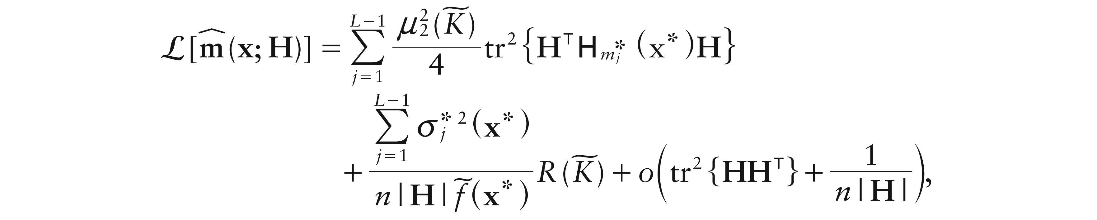
Hence, under the assumptions of Result, it is straightforward to see that asymptotic biases of the above estimators are the same as those obtained in Section 5 for local constant and local linear ones, respectively, with H_j in place of H, while for both estimators

Mvar [\overset{}{m} (x; H_{1,,} H_{L 1})]_{j 1}^{L 1} \frac{{\overset{}{}}_{j}^{2} (x^{*})}{n |H_{j}| \overset{}{f} (x^{*})} \{\overset{}{K} (z^{*})}^{2} d z^{*} o (_{j 1}^{L 1} \frac{1}{n |H_{j}|}) .

Finally, assuming H_jh_j I_D–1, the value of h_j minimizing the asymptotic version of $[\overset{}{m} (x; H_{1},, H_{L 1})]$ is

{\{\frac{(D 1) V_{j}}{{4 U}_{j}}\}}^{\frac{1}{D 3}} n^{\frac{1}{D 3}}

Remark 5. A Referee warned out that above described directional smoothing strategy could give place to difficulties of interpretation from the perspective of application because different smoothing in different ratios can result in predictions leaving the convex hull of the observations.

8 Real-data applications

We consider two real-data case studies on concentration of chemical elements using the Kola dataset. The Kola Ecogeochemistry Project (1992–1998) is an environmental investigation in Arctic Europe aimed both to study the impact of major industrial activities in the western Kola Peninsula and to obtain a regional mapping of heavy metals and pollution ecosystems. Samples of soil were taken in four different layers: moss, O-horizon, B-horizon and C-horizon. See Reimann et al. (1998) for details. The whole dataset is available in the package StatDA of the (see Filzmoser and Steiger, 2009).

8.1 Regression from IR to ³

We compare our non-parametric method with the linear parametric one introduced by Egozcue et al. (2012). In Egozcue et al. (2012), three chemical elements are considered: Fe (Iron), K (Potassium) and P (Phosphorus), all taken from the O-horizon layer of soil. They studied the concentration of these three elements as dependent on latitude, longitude and elevation of the examined soil, founding that elevation is the only highly significant predictor. On the basis of their results, we focus on simple regression, where the above minerals are explained only by elevation, say X. We use the same balances, or coordinates, as Egozcue et al. (2012):

Y_{1}^{*} \sqrt{\frac{2}{3}} \ln (\frac{Fe}{\sqrt{K . P}}), Y_{2}^{*} \frac{1}{\sqrt{2}} \ln (\frac{P}{K}) .

Denoting the ith observed response as ( $Y_{1 i}, Y_{2 i}$ ), we perform two separate regression estimates on ( $Y_{1 i}^{*}, X_{i}$ ) and ( $Y_{2 i}^{*}, X_{i}$ ), respectively. We use the simplicial Epanechnikov kernel, defined according to (3.1), and set two cross-validated smoothing parameters as follows:

\underset{h_{j}}{argmin}_{i 1}^{n} (Y_{ji}^{*} {\overset{}{m}}_{j (i)}^{*} (X_{i}; h_{j}))^{2}, j \{1, 2\}

where the estimate ${\overset{}{m}}_{j (i)}^{*}$ is performed after leaving the observation (X_i, Y_ji) out of the sample. For the local constant fit, we obtained (h₁140, h₂73.5), whereas for the local linear one, we got (h₁260, h₂105.7).

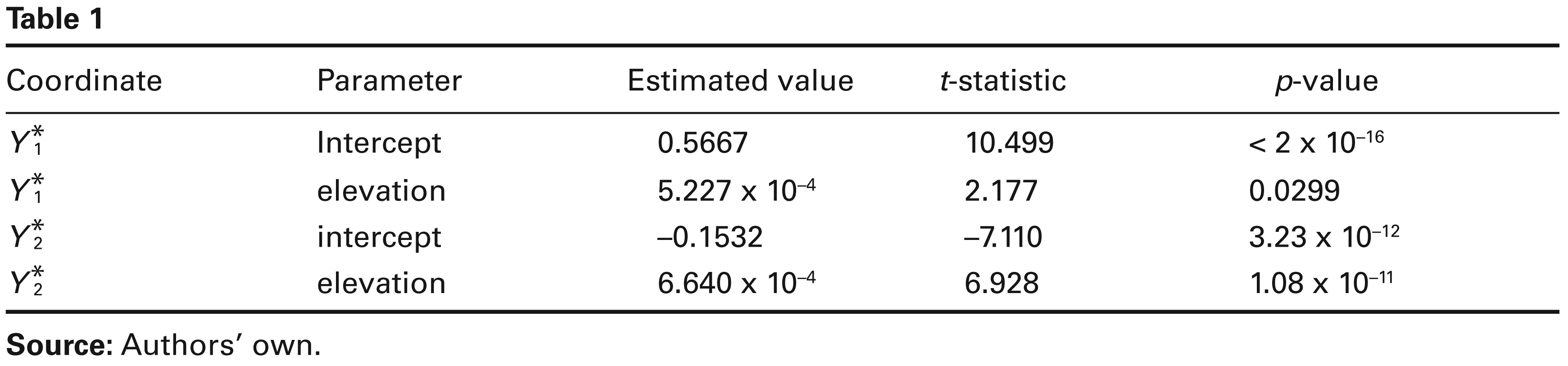
The simple, linear parametric estimate is summarized in Table 1:

Table 1
Authors’ own.

Coordinate	Parameter	Estimated value	t-statistic	p-value
$Y_{1}^{*}$	Intercept	0.5667	10.499	< 2 x 10^–16
$Y_{1}^{*}$	elevation	5.227 x 10^–4	2.177	0.0299
$Y_{2}^{*}$	intercept	–0.1532	–7.110	3.23 x 10^–12
$Y_{2}^{*}$	elevation	6.640 x 10^–4	6.928	1.08 x 10^–11

We can note that elevation is highly significant only for the coordinate $Y_{2}^{*}$ . Since Fe is notoriously independent from elevation, only P and K are responsible for such a significance. In particular, the ratio P over K increases with the elevation.

Figure 1

Source: Authors’ own.

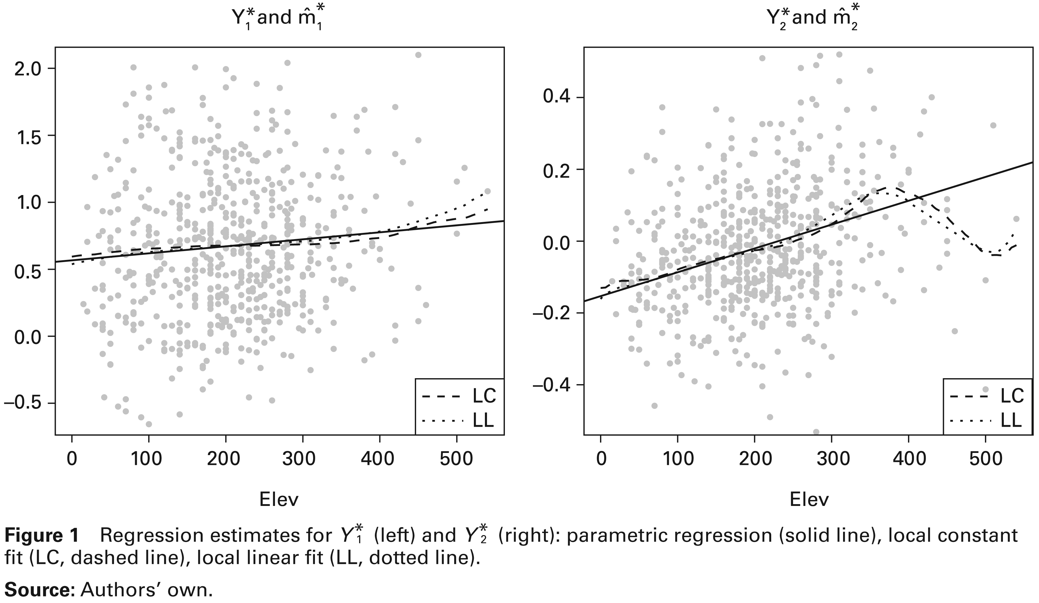
In Figure 1 (left), the parametric, local constant and local linear fits are represented for the $Y_{1}^{*}$ case. Our non-parametric estimators largely confirm the parametric one.

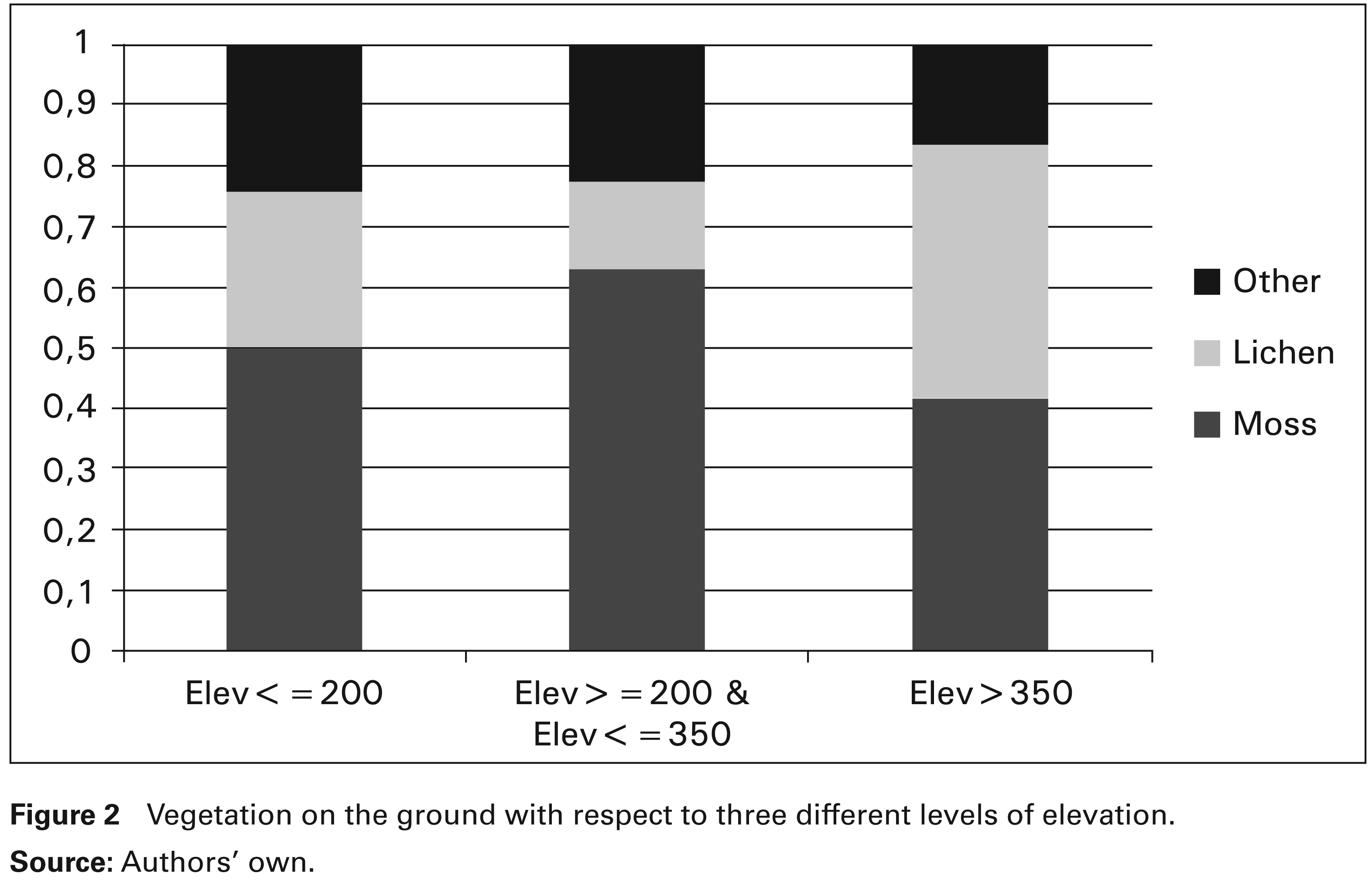
Coming at the second regression fit, where the log-ratio of P over K is the response, we do not observe the same agreement as before; see Figure 1 (right). Specifically, for elevations higher than 350 m, local fits show a decreasing trend, differently from the parametric method. Surely, the parametric linear regression is locally inadequate if we consider that only one out of the 10 observations with the highest elevation is above the straight line. Overall, we can affirm that the local method correctly detects a trend change. To understand the physical phenomenon underpinning such a trend change, we firstly investigated a possible relation between elevation and the lithology of the soil. Indeed, it doesn’t seem to be any relation between them in our data, while vegetation on the ground seem strictly related, as follows. The ground, in our case, is mainly composed of moss and lichens, see Figure 2. Now, the moss, which represents the majority of vegetation, first increases as elevation increases, but after 350 m, it exhibits a trend inversion. By contrast, the behaviour of lichens is opposite, first decreasing and then, after 350 m, reaching the same proportion as the moss. Now consider that moss is a green plant and lichens are a symbiosis of fungus and algae. Consequently, moss requires more phosphorus-over-potassium than lichens. In particular, phosphorus is a nutrient element for green plants, whereas potassium is present, in our case, as a mineral. Our conclusion here is that the presence of moss and lichens, when related to elevation, seems to confirm the trend of ${\overset{}{m}}_{2}^{*}$ .

Figure 2

Source: Authors’ own.

8.2 Regression from ³ to ³

As the second real-data case study, we present a regression where a three-part composition of the O-horizon layer (Sr (Strontium), Rb (Rubidium) and Ca (Calcium)) predicts a three-part composition of the moss layer (Mg (Magnesium), K (Potassium) and P (Phosphorus)). As a benchmark, we adopt a simple parametric approach made of two linear regressions based on ilr transformations.

We use the following balances:

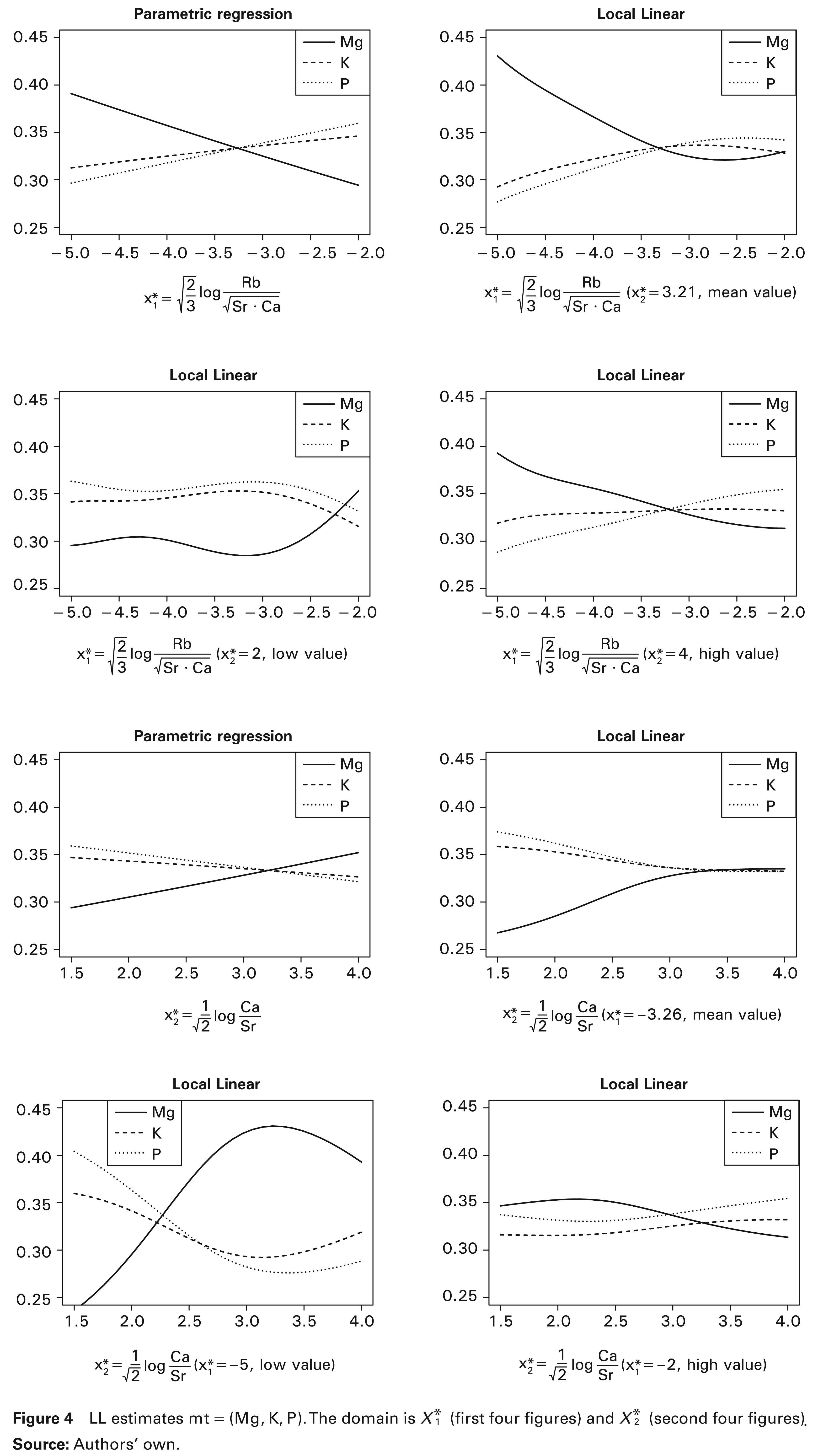
X_{1}^{*} \sqrt{\frac{2}{3}} \ln (\frac{Rb}{\sqrt{S r . Ca}}), X_{2}^{*} \frac{1}{\sqrt{2}} \ln (\frac{Ca}{Sr}),

Y_{1}^{*} \sqrt{\frac{2}{3}} \ln (\frac{\sqrt{K . P}}{Mg}), Y_{2}^{*} \frac{1}{\sqrt{2}} \ln (\frac{K}{P}) .

Applying the cross-validation criterion, the values obtained for the smoothing parameters of local linear estimators (with simplicial normal kernel) of the coordinates are h₁0.64 and h₂1.20, respectively. The plots in Figure 3 have ( $X_{1}^{*}$ , $X_{2}^{*}$ ) as domain and $Y_{1}^{*}$ (top) and $Y_{2}^{*}$ (bottom) as ordinate. Figure 4 considers $X_{1}^{*}$ (or $X_{2}^{*}$ ) as domain and the three components of Y(Mg, K, P) for particular values of $X_{2}^{*}$ ( $X_{1}^{*}$ respectively) as ordinate.

From Figure 3, we can see that, as general trend, $Y_{1}^{*}$ increases with $X_{1}^{*}$ , while $Y_{2}^{*}$ remains unchanged. The behaviour of $Y_{1}^{*}$ as dependent on $X_{1}^{*}$ can be explained by Figure 4, where we see that K and P grow while Mg decreases. Also, $Y_{1}^{*}$ decreases as $X_{1}^{*}$ increases, this happens because K and P decrease while Mg becomes higher. Similarly as before, $Y_{2}^{*}$ remains nearly constant with respect to $X_{2}^{*}$ .

From a geochemical point of view, the above trends can be motivated by observing that Rb and K have the same trend since the source of Rb is K-feldspar, and also that Ca and Mg are proportional as well since they are both bivalent, and in Ca-carbonate it is possible to have also Mg at 50%.

Some departures from the general trend are exhibited by the non-parametric fits as follows. First, $Y_{1}^{*}$ has a seemingly parabolic trend rather than linear, and it depends essentially on the behaviour of Mg. Moreover, when Rb is high—relative to its mean values—Mg does not increase with $X_{2}^{*}$ (essentially with Ca), but it is almost constant or tends to decrease. To find an explanation for this phenomenon, we have to look at the lithology of the ground.

In our samples, soils that are relatively rich in Rb are granitic, alkaline rocks, granulites or other igneous rocks. But these are poor in carbonates; therefore, an opposite trend between Ca and Mg seems to be natural. In fact, we have either minerals rich in Ca, or rich in Mg. This different behaviour of Ca and Mg in Rb-rich soils could not be grasped by linear parametric regression, while seems to be highlighted by our local fits.

Figure 3

Source: Authors’ own.

Figure 4

Source: Authors’ own.

9 Appendix

PROOF OF RESULT 1. Let ${ilr}_{U_{1}}$ and ${ilr}_{U_{2}}$ denote the ilr transformations corresponding to two different orthonormal bases for ^D, and let M₂(K) be the matrix in Equation (3.2) defined using ${ilr}_{U_{1}}$ . Moreover, let A be the orthogonal matrix of order D – 1, such that ${ilr}_{U_{2}} (x) A {ilr}_{U_{1}} (x)$ . Recalling that, by orthogonality of A, d ${(i l r}_{U_{2}} (x)) d {(i l r}_{U_{1}} (x))$ , it results.

_{^{D 1}} K (x) {ilr}_{U_{2}} (x) {ilr}_{U_{2}}^{} (x) d ({ilr}_{U_{2}} (x))_{^{D 1}} K (x) A {ilr}_{U_{1}} (x) {ilr}_{U_{1}}^{} (x) A^{} d ({ilr}_{U_{1}} (x))

A_{^{D 1}} K (x) {ilr}_{U_{1}} (x) {ilr}_{U_{1}}^{} (x) d ({ilr}_{U_{1}} (x)) A^{}

_{2} (\overset{}{K}) {AA}^{}

_{2} (\overset{}{K}) I_{D 1}

where the second identity holds because M₂(K) is a diagonal matrix, while the last one follows by orthogonality of A.

PROOF OF RESULT 2. Since $U^{} 1_{D} 0_{D 1}$ , and $_{g} (x) D_{\overset{}{g}} (x^{*}) U^{}$ , it results

_{g} (x) 1_{D} D_{\overset{}{g}} (x^{*}) U^{} 1_{D} 0

Now, because of $U^{} U I_{D 1}$ , and ${UU}^{} I_{D} D^{1} 1_{D} 1_{D}^{}$ , we have

\begin{matrix} D_{\overset{}{g}} (x^{}) u^{*}_{g} (x) {UU}^{} \ln (u) \\ _{g} (x) \ln (u) D^{1}_{g} (x) 1_{D} 1_{D}^{T} \ln (u) \\ _{g} (x) \ln (u). \end{matrix}

Footnotes

Acknowledgements

The authors are grateful to J.J. Egozcue, V. Pawlowsky-Glahn and R. Tolosana-Delgado for various useful discussions and suggestions. The authors also thank two Referees for their constructive comments which led to an improved presentation.

References

Aitchison

(1982) The statistical analysis of compositional data (with discussion). Journal of the Royal Statistical Society, Series B, 44, 139–77.

Aitchison

(1986) The statistical analysis of compositional data. Monographs on statistics and applied probability. (Reprinted 2003 with additional material by The Blackburn Press). London: Chapman & Hall Ltd., 416.

Aitchison

Bacon-Shone

(1984) Log contrast models for experiments with mixtures. Biometrika, 71, 323–30.

Aitchison

Lauder

(1985) Kernel density estimation for compositional data. Applied Statistics, 34, 129–37.

Barceló-Vidal

Martín-Fernandez

Mateu-Figueras

(2011) Compositional differential calculus on the simplex. In Pawlowsky-Glahn

Buccianti

, (eds). Compositional Data Analysis: Theory and Applications, Chichester UK: Wiley, 176–90.

Chacón

Mateu-Figueras

Martín-Fernández

(2011) Gaussian kernels for density estimation with compositional data. Computers & Geosciences, 37, 702–11.

Di Marzio

Panzera

Taylor

(2013) Non-parametric regression for circular responses. Scandinavian Journal of Statistics, 40, 238–55.

Di Marzio

Panzera

Taylor

(2014) Nonparametric regression for spherical data. Journal of the American Statistical Association, 109, 748–63.

Egozcue

Daunis-i-Estadella

Pawlowsky-Glahn

Hron

(2012) Simplicial regression. The normal model. Journal of Applied Probability and Statistics, 6, 87–108.

10.

Egozcue

Pawlowsky-Glahn

Mateu-Figueras

Barceló-Vidal

(2003) Isometric logratio transformations for compositional data analysis. Mathematical Geology, 35, 279–300.

11.

Filzmoser

Steiger

(2009) StatDA: Statistical Analysis for Environmental Data. R package version 1.1.

12.

Hijazi

Jernigan

(2009) Modelling compositional data using Dirichlet regression models. Journal of Applied Probability and Statistics, 4, 77–91.

13.

Hron

Filzmoser

Thompson

(2012) Linear regression with compositional explanatory variables. Journal of Applied Statistics, 39, 1115–28.

14.

Martín-Fernandez

Hron

Filzmoser

Palarea-Albaladejo

(2012) Modelbased replacement of rounded zeros in compositional data: Classical and robust approach. Computational Statistics & Data Analysis, 56, 2688–704.

15.

Pawlowsky-Glahn

Buccianti

(eds) (2011) Compositional Data Analysis. Theory and Applications. John Wiley & Sons Ltd.

16.

Pawlowsky-Glahn

Egozcue

(2001) Geometric approach to statistical analysis on the simplex. Stochastic Environmental Research and Risk Assessment (SERRA), 15, 384–98.

17.

Reimann

Äyräs

Chekushin

Bogatyrev

, (1988) Environmental geochemical atlas of the Central Barents Region. Geological Survey of Norway (NGU), Geological Survey of Finland (GTK) and Centrl Kola Expedition (CKE). Special publication, Trondheim, Espoo, Monchegorsk.

18.

Ruppert

Wand

(1994) Multivariate locally weighted least squares regression. The Annals of Statistics, 22, 1346–70.

19.

Scheffè

(1958) Experiments with mixtures. Journal of the Royal Statistical Society, Series B, 22, 344–60.

20.

Scheffè

(1963) The simplex-centroid design for experiments with mixtures. Journal of the Royal Statistical Society, Series B, 22, 235–63.

21.

Tolosana-Delgado

Van Den Boogart

(2011) Linear models with compositions in R. In Pawlowsky-Glahn

Buccianti

, eds, Compositional Data Analysis: Theory and Applications, Chichester, UK: Wiley, 356–71.

Non-parametric regression for compositional data

Abstract

Keywords

1 Introduction

2 Preliminaries

3 Kernels on the simplex

8.1 Regression from IR to 3

Table 1 Authors’ own.

Footnotes

Acknowledgements

References

8.1 Regression from IR to ³

Table 1
Authors’ own.