Two Cholesky-log-GARCH models for multivariate volatilities

Abstract

Parsimonious estimation of high-dimensional covariance matrices is of fundamental importance in multivariate statistics. Typical examples occur in finance, where the instantaneous dependence among several asset returns should be taken into account. Multivariate GARCH processes have been established as a standard approach for modelling such data. However, the majority of GARCH-type models are either based on strong assumptions that may not be realistic or require restrictions that are often too hard to be satisfied in practice. We consider two alternative decompositions of time-varying covariance matrices $Σ_{t}$ . The first is based on the modified Cholesky decomposition of the covariance matrices and second relies on the hyperspherical parametrization of the standard Cholesky factor of their correlation matrices $R_{t}$ . Then, we combine each Cholesky factor with the log-GARCH models for the corresponding time–varying volatilities and use a quasi maximum likelihood approach to estimate the parameters. Using log-GARCH models is quite natural for achieving the positive definiteness of $Σ_{t}$ and this is a novelty of this work. Application of the proposed methodologies to two real financial datasets reveals their usefulness in terms of parsimony, ease of implementation and stresses the choice of the appropriate models using familiar data-driven processes such as various forms of the exploratory data analysis and regression.

Keywords

Cholesky decomposition Covariance matrix GARCH model hyperspherical coordinates volatility

Received October 2013; revised June 2014; accepted June 2014

1 Introduction

During the last three decades, parsimonious modelling of covariance structures has received increasing attention (Engle, 1982; Engle, 2002; Tsay, 2010). The two important challenges in modelling covariance matrices are:

The positive definiteness of a covariance matrix $Σ$ .

The high-dimensionality (complexity) where the number of parameters grows quadratically with the number of variables.

In particular, for a collection of

m \times m

covariance matrices

Σ_{i}, i = 1, \dots, n

, one has to deal with

nm (m + 1) / 2

constrained parameters. Hence, as

m

and

n

increase, computation and efficient estimation of

Σ_{i}

’s become daunting tasks. A typical example is the case of multivariate volatility in finance (see, e.g., Bollerslev, 1990; Engle, 2002) where

m

is the number of assets in a portfolio and

n

, the number of covariances to be estimated, is the same as the length of the time series of returns.

Several multivariate extensions of the univariate GARCH models (Bollerslev, 1986) have been proposed in the finance literature. Early variants of multivariate GARCH (MGARCH) models (Engle and Kroner, 1995) heavily depend upon a growing number of free parameters. Simplifications can occur when the coefficients are diagonal matrices (Alexander, 2001 Chap. 7), but then complicated restrictions on the coefficient parameters are required to ensure their positive definiteness. Meanwhile many overparameterized variants of MGARCH models for financial time series have been developed (Francq and Zakoian, 2010 Chap. 11, for example). Most of them are either based on strong assumptions that may not be realistic (for instance, the assumption of constant correlation of the CCC-GARCH model) or require restrictions that are often too hard to be satisfied in practice.

The two challenges of modelling a covariance model can be resolved simultaneously by relying on the idea of Cholesky decomposition which provides statistically meaningful and unconstrained parameterizations and guarantees the positive definiteness of the estimated covariance matrix (Pourahmadi, 1999, 2011). While the bulk of early applications of the Cholesky decomposition based covariance modelling has been to longitudinal data arising from health sciences, examples of using Cholesky decomposition for the estimation of multivariate volatilities remain rather sparse, see Dellaportas and Pourahmadi, 2004; Dellaportas and Pourahmadi, 2012, Tsay (2010, Chap. 10), Chang and Tsay6, 2010 and Lopes et al., 2012.

Even though the (modified) Cholesky decomposition (MCD) provides unconstrained and statistically interpretable parameterization of a covariance matrix, its drawback is that the innovation variances are not the same as the (marginal) volatilities of the assets’ returns in a portfolio. Fortunately, using the variance-correlation decomposition

Σ = H R H,

(1.1)

where

H = diag (σ_{1}, \dots, σ_{m})

, allows one to model separately the variances and correlations of the asset returns. However, since the diagonal entries of a correlation matrix are equal to one, the nonredundant entries of the Cholesky factor of the correlation matrix

R

are constrained. Surprisingly, this new challenge is mitigated by reparameterizing the Cholesky factor of

R

using the hyperspherical coordinates as in Rebonato and Jäckel, 2000 and subsequently employed by (Creal et al., 2011) and Zhang et al., 2014.

In this article we introduce two classes of models based on the Cholesky decompositions of a covariance matrix and its correlation matrix. The first class of models is based on the MCD of $Σ$ , and the second is based on the standard Cholesky decomposition of $R$ in (1.1) and the hyperpherical parametrization (HPC) of its Cholesky factor. We rely on the log-GARCH models (Geweke, 1986; Francq et al., 2013) for their time-varying innovation and marginal variances. It is shown that using log-GARCH models is quite natural for achieving the positive definiteness of $Σ$ .

The remainder of the article is organized as follows: In Section 2 we shall briefly review the literature on multivariate GARCH models for financial time series. Section 3 introduces the two proposed modelling approaches based on MCD and HPC. Applications to financial data series follow in Section 4. Section 5 concludes the article and outlines future research.

2 Multivariate GARCH models

Multivariate GARCH (MGARCH) models have been surveyed by many authors, see, for instance, Silvennoinen and Teräsvirta, 2009 and Francq and Zakoian, 2010 among others. Here, we avoid mathematical details and confine ourselves to a discussion of the pros and cons of different MGARCH models.

In principle, the major problem of MGARCH models is that the number of parameters grows rapidly with the dimension of the multivariate process. Hence, estimation of such models becomes quite challenging in practice because of numerical complications when optimizing a likelihood function with a large number of constrained parameters. In fact, in such cases ensuring the positive definiteness of the conditional covariance matrix is often infeasible in practice. Hence models are defined in a way that the property of positive definiteness is implicitly implied (Silvennoinen and Teräsvirta, 2009).

In what follows, we focus on three major classes of MGARCH models. The first class arises as a direct generalization of the univariate GARCH model (VEC and BEKK models). The models in the second class can be thought as linear combinations of univariate GARCH models (factor GARCH, principal component GARCH models). The third class consists of non-linear combinations of univariate GARCH models, i.e., the constant conditional correlation and dynamic conditional correlation models and their extensions.

The VEC-GARCH model (Bollerslev et al., 1988) assumes that every conditional variance and covariance is a function of lagged conditional variances and covariances as well as lagged squared returns and cross-products of returns. Though this formulation makes the VEC model very flexible, there exist only restrictive sufficient conditions for the covariance matrix to be positive definite for all $t$ . Moreover, the number of parameters increases rapidly with dimensionality and parameters estimation is computationally demanding. Positive definiteness of the conditional covariance matrix can be achieved under the assumption of a diagonal-VEC model (Bollerslev et al., 1988). However, this particular version does not allow for potential interactions among various conditional variances and covariances. The BEKK model of Engle and Kroner, 1995 is another restricted version of the VEC model. The main advantage of this specification is that the positive definiteness constraint is satisfied by its construction. However, this model suffers from identifiability issues and there exist difficulties in the estimation and interpretation of the model parameters.

The general idea of factor models is that the observations are generated by underlying factors that are conditionally heteroskedastic and have a GARCH structure. This allows the dimensionality of the problem to be reduced when the number of factors is small relative to the dimension of the return vector (Silvennoinen and Teräsvirta, 2009). In this context, the first factor model was introduced by Engle et al., 1990 and its structure implies that the factors are generally correlated. Often, this property may prove undesirable in practice since different factors may capture similar characteristics of the data. To overcome this limitation, several factor models with uncorrelated factors have been proposed in the literature, see e.g., the Full Factor (FF-) GARCH model of Vrontos et al., 2003.

The constant conditional correlation (CCC) and dynamic conditional correlation (DCC) GARCH models are representative examples of models which are based on (1.1). For the CCC-GARCH model (Bollerslev, 1990), the conditional correlation matrix is assumed to be time-invariant. This assumption may be quite restrictive and unrealistic in practice. The dynamic conditional correlation (DCC-) GARCH model of Engle, 2002 and the Varying Correlation (VC-) GARCH model of Tse and Tsui, 2002 are similar specifications that impose GARCH-type dynamics on the conditional correlation matrices. These models have also certain drawbacks, as for example the correlation processes are restricted to have the same dynamic structure, or leading to invalid correlation matrices.

3 The proposed methodology

In this section we discuss in detail the two classes of models based on the Cholesky decomposition of a covariance matrix and its corresponding correlation matrix. In both instances, we employ log-GARCH models for the relevant time-varying volatilities. We start this section with a short review of log-GARCH models.

3.1 The log-GARCH models

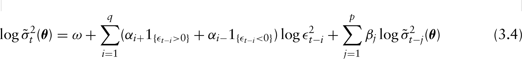
The (asymmetric) log-GARCH( $p$ , $q$ ) model is defined as (Geweke, 1986):

\begin{matrix} ε_{t} & = & σ_{t} η_{t} \\ log σ_{t}^{2} & = & ω + \sum_{i = 1}^{q} (α_{i +} 1_{{ε_{t - i} > 0}} + α_{i -} 1_{{ε_{t - i} < 0}}) log ε_{t - i}^{2} + \sum_{j = 1}^{p} β_{j} log σ_{t - j}^{2} \end{matrix}

(3.1)

where

σ_{t} > 0

and

η_{t}

is a sequence of independent and identically distributed (i.i.d.) variables with

E η_{0} = 0

and

E η_{0}^{2} = 1

. When

α_{+} = α_{-}

with

α_{+} = (α_{1 +}, \dots, α_{q +})

and

α_{-} = (α_{1 -}, \dots, α_{q -})

, the usual symmetric log-GARCH model is obtained.

Evidently, this formulation allows for asymmetries between positive and negative asset returns, i.e., the so-called leverage effect, and it does not impose any positivity restrictions on the volatility coefficients (Francq et al., 2013). Other interesting features of the log-GARCH specification are (i) the absence of a lower bound for the volatility, (ii) persistent effects of both large and small shocks on the volatility and (iii) compatibility under power transformations of the absolute observations. For recent works on this class of models, the reader is referred to Francq et al., 2013.

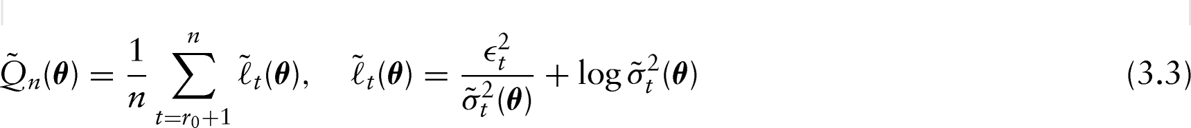
Estimates of the log-GARCH parameters are obtained by Quasi Maximum Likelihood (QML). In particular, a quasi maximum likelihood estimator (QMLE) of the vector of unknown parameters $θ$ is defined as any solution ${\hat{θ}}_{n}$ of:

{\hat{θ}}_{n} = arg min_{θ \in Θ} {\tilde{Q}}_{n} (θ),

(3.2)

where

{\tilde{Q}}_{n} (θ) = \frac{1}{n} \sum_{t = r_{0} + 1}^{n} {\tilde{ℓ}}_{t} (θ), {\tilde{ℓ}}_{t} (θ) = \frac{ε_{t}^{2}}{{\tilde{σ}}_{t}^{2} (θ)} + log {\tilde{σ}}_{t}^{2} (θ)

(3.3)

with

r_{0}

being a fixed integer and

log {\tilde{σ}}_{t}^{2} (θ)

recursively defined by

log {\tilde{σ}}_{t}^{2} (θ) = ω + \sum_{i = 1}^{q} (α_{i +} 1_{{ε_{t - i} > 0}} + α_{i -} 1_{{ε_{t - i} < 0}}) log ε_{t - i}^{2} + \sum_{j = 1}^{p} β_{j} log {\tilde{σ}}_{t - j}^{2} (θ)

(3.4)

for

t = 1, \dots, n

. In what follows, we restrict out attention to simple model (3.4) with

p = q = 1

. Francq et al., 2013 show that the asymptotic behaviour of the QMLE is not affected by the choice of the initial values. However, the finite sample estimate of

{\hat{θ}}_{n}

is quite sensitive to these initial values. For the applications discussed in Section 4, initial values have been obtained by fitting linear least squares regression models to the sample of log variances obtained by a moving blocks approach.

Proofs of strong consistency and asymptotic normality of the QMLE ${\hat{θ}}_{n}$ are discussed by Francq et al., 2013.

3.2 The Cholesky decomposition of a covariance matrix

We use the fact that a symmetric matrix $Σ$ is positive definite if and only if there exists a unique lower triangular matrix $T$ , with 1’s as diagonal entries, and a unique diagonal matrix $D$ with positive diagonal entries such that (Pourahmadi, 1999)

T Σ T^{'} = D .

(3.5)

The entries of

T

and the logarithms of the diagonal of

D

are unconstrained and interpretable as regression coefficients and prediction (innovation) variances when regressing a measurement on its predecessors as explained next.

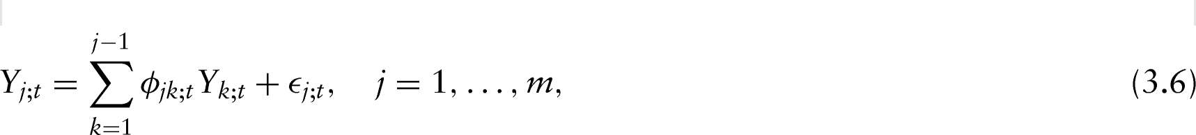
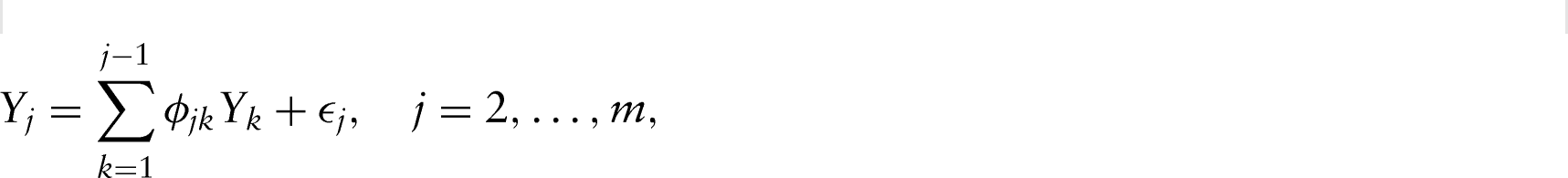
In financial applications, due to the presence of time-varying volatilities, a different covariance matrix $Σ_{t}$ has to be estimated at each time point $t = 1, \dots, n$ . For reparameterization of $Σ_{t}$ using (3.5) and interpretation of the entries of the matrices $T_{t}$ and $D_{t}$ , one may rely on the idea of regression as in Pourahmadi, 1999 and (Tsay, 2010). More specifically, for a given time point $t$ , let $Y_{t} = (Y_{1; t}, \dots, Y_{m; t})$ be a multivariate normal random vector with mean zero and positive-definite covariance matrix $Σ_{t}$ , where $m$ is the dimension of the multivariate series. The linear least squares regression of $Y_{j; t}$ , $j = 1, \dots, m$ on its predecessors $Y_{1; t}, \dots, Y_{j - 1; t}$ , is defined as:

Y_{j; t} = \sum_{k = 1}^{j - 1} ϕ_{jk; t} Y_{k; t} + ε_{j; t}, j = 1, \dots, m,

(3.6)

where the regression coefficients

ϕ_{jk; t}

determined from

Σ_{t}

are unconstrained. The prediction error (innovation)

ε_{j; t}

has variance

Var (ε_{jt}) = d_{j; t}^{2}

and the successive prediction errors are uncorrelated so that the covariance matrix of

ϵ_{t} = (ϵ_{1; t}, \dots, ϵ_{m; t})'

is diagonal and given by

D_{t} = cov (ε_{t}) = diag (d_{1; t}^{2}, \dots, d_{m; t}^{2})

. The

m

regression models in (3.6) can be written in a matrix form as:

ε_{t} = T_{t} Y_{t},

where

T_{t}

is a unit lower triangular matrix with

- ϕ_{jk; t}

in the (

j, k

)th position, for

j = 2, \dots, m

and

k = 1, \dots, j - 1

. Then, it follows that the unit lower triangular matrix

T_{t}

diagonalizes

Σ_{t}

as in (3.5) such that:

T_{t} Y_{t} \equiv ε_{t} \sim N (0, D_{t}) .

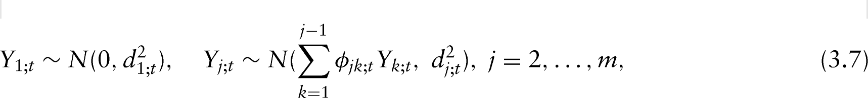
Obviously, the joint normal distribution of

Y_{t}

can be expressed as a set of

m

recursive conditional regressions:

Y_{1; t} \sim N (0, d_{1; t}^{2}), Y_{j; t} \sim N (\sum_{k = 1}^{j - 1} ϕ_{jk; t} Y_{k; t}, d_{j; t}^{2}), j = 2, \dots, m,

(3.7)

where

ϕ_{jk; t}

and

log d_{j; t}^{2}

are unconstrained, and one may model them using either difference equations or covariates (Pourahmadi, 1999). In this article, we model the prediction (innovation) variances

log d_{j; t}^{2}

using log-GARCH models defined recursively in time by,

log d_{j; t}^{2} = λ_{0} + {λ_{1} 1_{{ε_{j; t - 1} > 0}} + λ_{2} 1_{{ε_{j; t - 1} < 0}}} log ε_{j; t - 1}^{2} + λ_{3} log d_{j; t - 1}^{2}, j = 1, \dots, m,

(3.8)

so that (3.7) and (3.8) define our stochastic volatility model. The log-GARCH model (3.8) is a reasonable choice since

it helps to achieve the positive definiteness of the covariance matrix $Σ_{t}$ by guaranteeing that the diagonal entries of $D_{t}$ ’s are positive, and

it allows for asymmetric effects between positive and negative latent factors, and incorporates information from the past reflecting the time-varying nature of the data.

Using the idea of generalized linear models and employing covariates as in (Pourahmadi, 1999) one may write:

ϕ_{jk; t} = g (w_{jk; t}, γ), log d_{j; t}^{2} = υ (z_{j; t}, λ),

(3.9)

where

g (\cdot, \cdot)

and

υ (\cdot, \cdot)

are functions,

w_{jk; t}

and

z_{j; t}

are

q_{1} \times 1

and

q_{2} \times 1

vectors of covariates,

γ = {(γ_{1}, \dots, γ_{q_{1}})}^{'}

and

λ = {(λ_{1}, \dots, λ_{q_{2}})}^{'}

are unknown parameters for the regression coefficients and innovation variances, respectively. Parameteric models for

g (\cdot, \cdot)

and

υ (\cdot, \cdot)

and suitable covariates involving powers of time and time-lag can be identified using a data-driven process based on regressograms (Pourahmadi, 1999; Pourahmadi, 2000). These are useful tools for reducing the high number of parameters involved in modelling many large covariance matrices. The optimum degrees of the respective polynomials can be identified using the BIC-based model selection criterion proposed by Pan and MacKenzie, 2003. Semiparametric and nonparametric models have also received some interest in recent years (see, e.g., Lin and Ying, 2001; Pan et al., 2009; Leng et al., 2010).

The high number of parameters in $T_{t}$ due to its time-dependence can be further reduced by replacing them with a specific time-invariant lower triangular matrix $T$ , such as exchangeable (compound symmetry), AR(1) and general Toeplitz matrices, see Dellaportas and Pourahmadi, 2004; Dellaportas and Pourahmadi, 2012 Dellaportas and Pourahmadi, 2004; Dellaportas and Pourahmadi, 2012 for more examples. Interestingly, in spite of this simplifying assumption, the time-varying nature of the diagonal matrices $D_{t}$ ’s lead to bona fide time-varying correlation matrices for the asset returns in finance.

We estimate the time-invariant parameters of $T = (ϕ_{jk})$ by fitting successive regression models of the form:

Y_{j} = \sum_{k = 1}^{j - 1} ϕ_{jk} Y_{k} + ε_{j}, j = 2, \dots, m,

to the columns of the

n \times m

data matrix. A drawback of this approach is that it requires ordering the

m

stocks in a portfolio. The interested reader is referred to Dellaportas and Pourahmadi, 2004; Dellaportas and Pourahmadi, 2012 Dellaportas and Pourahmadi, 2004; Dellaportas and Pourahmadi, 2012 Dellaportas and Pourahmadi, 2004; Dellaportas and Pourahmadi, 2012 for a thorough discussion on the role and impact of ordering the variables on the Cholesky decomposition. In the sequel, we adopt their suggestion using the BIC as a decision tool for ordering the stocks. Hence, assuming that the vector

Y

consists of the ordered stocks (or series under study),

{\hat{ϕ}}_{jk}

’s are the ordinary least squares coefficients obtained after regressing

Y_{j}

Y_{1}, \dots, Y_{j - 1}

(no intercept regression models).

Of course, once $ϕ_{jk; t} \equiv ϕ_{jk}$ ’s and $d_{j; t}^{2}$ ’s or $T$ and $D_{t}$ are available then we construct $Σ_{t} = T^{- 1} D_{t} {(T^{- 1})}^{'}$ which is guaranteed to be positive-definite. For estimation of the vector of unknown parameters $λ$ , we employ a QML approach, as explained by (3.2)-(3.4), after substitution of ${\tilde{σ}}_{t}^{2}$ by ${\tilde{d}}_{j; t}^{2}$ and $θ$ by $λ$ .

3.3 Hyperspherical parametrization of the Cholesky factor of a correlation matrix

Unfortunately, the entries of the diagonal matrix $D$ in the modified Cholesky decomposition (MCD) of a covariance matrix as the regression error (innovation) variances, have the following two disadvantages:

they are different from the diagonal entries of $Σ$ or the volatilities of the assets which are of central importance in finance,

they depend on the order of the stocks or the variables in a random vector.

To explain this point further consider, for example, the bivariate case where the modified Cholesky decomposition is equivalent to performing a linear transformation from

Y_{t} = (Y_{1; t}, Y_{2; t})

ε_{t} = (ε_{1; t}, ε_{2; t})

where

ε_{1; t} = Y_{1; t}

ε_{2; t} = Y_{2; t} - ϕ_{21; t} Y_{1; t}

with

cov (ε_{t}) = D_{t} = diag (d_{1; t}^{2}, d_{2; t}^{2})

. Then, model (3.8), or even more generally model (3.9), refers to the log-variances of the prediction errors

ε_{t}

, not to the variances of the two original variables in

Y_{t}

In this section, we handle both problems by first separating the variances and correlations of $Y_{t}$ using the variance-correlation factorization (1.1), and then relying on the Cholesky decomposition of the correlation matrix $R_{t}$ . However, it should be pointed out that modelling the Cholesky factor of a correlation matrix using covariates is more difficult since its nonredundant entries are no longer unconstrained and guaranteeing that the diagonal entries of $R_{t}$ to be equal to $1$ , for $t = 1, \dots, n$ , is a new challenge.

Fortunately, the hyperspherical parameterization of the Cholesky factor of a correlation matrix addresses the aforementioned problems simultaneously (Rebonato and Jäckel, 2000). In particular, let $Y_{t} = (Y_{1; t}, \dots, Y_{m; t})$ be a generic random $m$ -vector with mean zero and positive–definite covariance matrix $Σ_{t} = H_{t} R_{t} H_{t}$ , where $H_{t} = diag (σ_{1; t}, \dots, σ_{m; t})$ is the diagonal matrix of standard deviations and $R_{t} = {(R_{jk; t})}_{j, k = 1}^{m}$ is the correlation matrix of $Y_{t}$ with $R_{jk; t} = corr (Y_{j; t}, Y_{k; t})$ . Consider the standard Cholesky decomposition of $R_{t}$ as follows:

R_{t} = B_{t} B_{t}^{'},

(3.10)

where

B_{t}

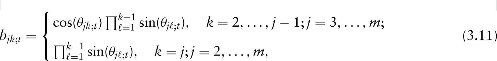
is a lower triangular matrix. It is known that its entries can be parameterized as

b_{11; t} = 1

b_{j 1; t} = cos (θ_{j 1; t})

j = 2, \dots, m

and:

b_{jk; t} = \{\begin{matrix} cos (θ_{jk; t}) \prod_{ℓ = 1}^{k - 1} sin (θ_{j ℓ; t}), k = 2, \dots, j - 1; j = 3, \dots, m; \\ \prod_{ℓ = 1}^{k - 1} sin (θ_{j ℓ; t}), k = j; j = 2, \dots, m, \end{matrix}

(3.11)

where

θ_{j ℓ; t}

’s are some angles in

[0, π)

(Rapisarda et al., 2007). The factorization (3.10) and the subsequent parametrization have several merits; the most important among them is that

B_{t} B_{t}^{'}

is always non-negative definite, satisfying the requirement of a correlation matrix with unit diagonal entries. Moreover, the angles

θ_{jk; t}

are unconstrained parameters in the range

[0, π)

in the sense that they are not functionally related to each other. Hence, this hyperspherical specification approach for a correlation matrix holds all of the nice features of a modified Cholesky decomposition of a covariance matrix.

This method was proposed by Rebonato and Jäckel, 2000 as a way to construct valid correlation matrices. Since then, only a few applications of the method have appeared in the literature where most of them are concerned with generating random correlation matrices rather than their parsimonious modelling. The work of Creal et al., 2011 which combines this parametrization with the idea of Generalized Autoregressive Score models, allows the angles $θ_{jk; t}$ to be time-varying and is focused on estimation and prediction with applications in finance. Recently, Zhang et al., 2014 have proposed a joint mean–variance correlation modelling approach using covariates for longitudinal data via hyperspherical parametrization of its Cholesky factor as above.

To parsimoniously model the variances and correlations of $Y_{t}$ , it is plausible to follow a setting similar to (3.7)–(3.9). In particular, the angles $θ_{jk; t}$ and variances $log σ_{j; t}^{2}$ can be modelled in terms of covariates as:

θ_{jk; t} = h (v_{jk; t}, ξ), log σ_{j; t}^{2} = s (u_{j; t}, κ),

where

h (\cdot, \cdot)

and

s (\cdot, \cdot)

are functions,

v_{jk; t}

and

u_{j; t}

are

p_{1} \times 1

and

p_{2} \times 1

generic vectors of covariates, and

ξ = (ξ_{1}, \dots, ξ_{p_{1}})'

and

κ = (κ_{1}, \dots, κ_{p_{2}})'

are unknown parameters corresponding to the dependence and variance respectively. The choice of the functions

h (\cdot, \cdot)

and

s (\cdot, \cdot)

is motivated by concepts similar to those described in Section 3.2 regarding the choice of

g (\cdot, \cdot)

and

υ (\cdot, \cdot)

, respectively. In particular, Zhang et al., 2014 have suggested using an analogue of the regressograms to identify the shape or pattern of

h (\cdot)

In Section 4 we start by letting the lower triangular matrix $B_{t}$ be time-invariant, i.e.,\ $B_{t} = B = (b_{jk})$ , which amounts to working with time-invariant or constant conditional correlation (CCC) matrices (Bollerslev, 1990). In this case, the elements of $B$ or the corresponding angles are estimated by simply substituting the sample correlation matrix $\hat{R}$ in (3.10). However, the log-GARCH model (3.1) will be used for handling the time-varying variances of the assets:

log σ_{j; t}^{2} = κ_{0} + {κ_{1} 1_{{Y_{j; t - 1} > 0}} + κ_{2} 1_{{Y_{j; t - 1} < 0}}} log Y_{j; t - 1}^{2} + κ_{3} log σ_{j; t - 1}^{2} .

(3.12)

Thus, the estimation of

Σ_{t}

is reduced to estimating the parameters

κ = (κ_{0}, κ_{1}, κ_{2}, κ_{3})

Estimation of a time-varying correlation matrix using the hyperspherical specification approach requires minimization of minus the log-likelihood

\begin{matrix} ℓ (ξ, κ) & = & - \frac{1}{2} \{\sum_{t = 1}^{n} log | H_{t} {\hat{R}}_{t} H_{t} | + \sum_{t = 1}^{n} Y_{t}^{'} H_{t}^{- 1} {\hat{R}}_{t}^{- 1} H_{t}^{- 1} Y_{t}\} \\ = & - \frac{1}{2} \sum_{t = 1}^{n} \sum_{j = 1}^{m} \{log σ_{j; t}^{2} + log B_{jj; t}^{2} + ε_{j; t}^{2}\}, \end{matrix}

where

ε_{j; t}

is the

j

th element of the

m \times 1

vector

ε_{t} = (ϵ_{1; t}, \dots, ϵ_{m; t})' = B_{t}^{- 1} H_{t}^{- 1} Y_{t}

and

ε_{1; t}, \dots, ε_{m; t}

are i.i.d.

N (0, 1)

. For this purpose an iterative Newton-Raphson algorithm can be employed.

Assuming that $B_{t} \equiv B$ (i.e., time-invariant), minimization of $- ℓ (ξ, κ) \equiv - ℓ (κ)$ only requires derivation of the score and expectation of the Hessian with respect to $κ$ . It can be shown that the score and the expectation of the Hessian are given by:

U (κ) = \frac{1}{2} \sum_{t = 1}^{n} Z_{t} (diag {R_{t}^{- 1} H_{t}^{- 1} Y_{t} Y_{t}^{'} H_{t}^{- 1}} - 1_{m}),

and

I (κ) = \frac{1}{4} \sum_{t = 1}^{n} Z_{t}^{'} (I_{m} + R_{t}^{- 1} \circ R_{t}) Z_{t},

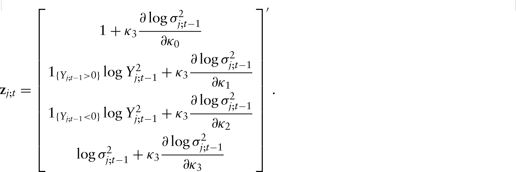
respectively, where

\circ

denotes the Hadamard product,

R_{t} \equiv R

and

R_{t} \equiv R

and

Z_{t} = {[{z^{'}}_{1; t}, \dots, {z^{'}}_{m; t}]}^{'}

is the

m \times 4

matrix of the first derivatives

z_{j; t}

of the right-hand side of (3.12),

z_{j; t} = {[\begin{matrix} 1 + κ_{3} \frac{\partial log σ_{j; t - 1}^{2}}{\partial κ_{0}} \\ 1_{{Y_{j; t - 1} > 0}} log Y_{j; t - 1}^{2} + κ_{3} \frac{\partial log σ_{j; t - 1}^{2}}{\partial κ_{1}} \\ 1_{{Y_{j; t - 1} < 0}} log Y_{j; t - 1}^{2} + κ_{3} \frac{\partial log σ_{j; t - 1}^{2}}{\partial κ_{2}} \\ log σ_{j; t - 1}^{2} + κ_{3} \frac{\partial log σ_{j; t - 1}^{2}}{\partial κ_{3}} \end{matrix}]}^{'} .

i.e.,Estimates of the parameters

κ

are obtained by applying a quasi-Fisher scoring algorithm as in Zhang et al., 2014. More specifically, at the

i

th iteration, we compute:

κ^{(i)} = κ^{(i - 1)} + {[I {(κ)}^{- 1} U (κ)] |}_{κ = κ^{(i - 1)}},

and the process is repeated till a pre-specified convergence criterion is satisfied. As an example of such a criterion, we have selected

∥ κ^{(i + 1)} - κ^{(i)} ∥

being less than

10^{- 6}

in absolute value. The starting values

κ^{(0)}

for the initialization of the algorithm are obtained by fitting log-GARCH(1,1) models to the crude variances estimated by the moving blocks approach and averaging the estimates obtained by these

m

models.

Note however that only convergence to a local optimum can be guaranteed, since the likelihood function is not globally convex.

4 Application

The forecast performance of the methods discussed in the previous section is illustrated using two financial data examples. The first dataset consists of a trivariate series of $n = 2275$ daily log returns while the second dataset comprises $n = 251$ monthly stock returns of 12 different US bluechips.

Apart from the suggested Cholesky decomposition and hyperspherical specification approaches, the constant conditional correlation (CCC) (Bollerslev, 1990) and the dynamic conditional correlation (DCC) (Engle, 2002) models of order (1,1) were used for comparison purposes. For the estimation of the CCC- and DCC-GARCH models, we used the ccc.estimation() and dcc.estimation() functions in R, respectively. Numerical algorithms for estimation through the Cholesky decomposition and hyperspherical specification approaches are described below in detail.

Figure 1:

Authors’ own.

Since the true realized covariance matrix is unknown, we employ a moving blocks approach (Lopes et al., 2012) to get a reliable proxy. In particular, at each time $t$ , we compute the sample covariance ${\tilde{Σ}}_{t}$ of $q$ observations centred at $t$ . At both the left and right end of the data range, the block size is truncated when it exceeds the observed time window. In what follows, we refer to the estimates obtained by the moving blocks approach as crude estimates.

Figure 2:

Authors’ own.

As already noted, we confine ourselves to the estimation of time-varying matrices $D_{t}$ and $H_{t}$ whilst assuming time-invariant matrices $T$ and $B$ in (3.5) and (3.10), respectively. With regard to the Cholesky decomposition approach, estimates of the elements of $T$ are obtained by successive linear least squares regressions of the ordered (according to BIC) $Y_{j}$ ’s on their predecessors $Y_{1}, \dots, Y_{j - 1}$ (see (3.6)). To obtain a sample of $D_{t}$ ’s, $t = 1, \dots, n$ , a similar procedure is followed within each block. Then, the log-GARCH(1,1) model (3.8) is fitted to the crude estimates $log {\tilde{d}}_{j; t}^{2}$ ’s providing the vector of estimated parameters $\hat{λ}$ through QMLE (Francq et al., 2013).

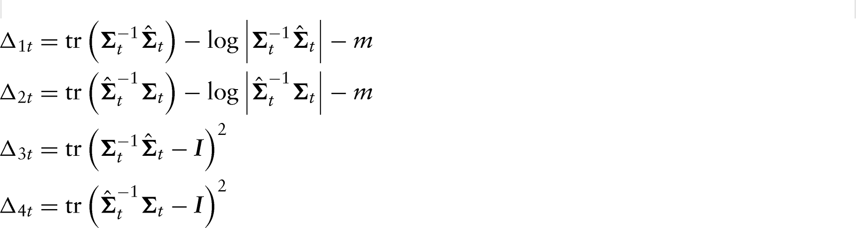
To measure the accuracy of a covariance matrix estimate ${\hat{Σ}}_{t}$ , we consider as a benchmark the moving blocks approach (i.e., $Σ_{t} \equiv {\tilde{Σ}}_{t}$ ) and calculate the commonly used entropy loss $Δ_{1 t}$ , the Kullback–Leibler loss $Δ_{2 t}$ and two quadratic loss functions $Δ_{3 t}$ and $Δ_{4 t}$ , see Chang and Tsay, 2010:

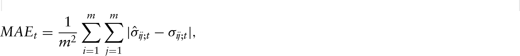
\begin{matrix} Δ_{1 t} & = & tr (Σ_{t}^{- 1} {\hat{Σ}}_{t}) - log |Σ_{t}^{- 1} {\hat{Σ}}_{t}| - m \\ Δ_{2 t} & = & tr ({\hat{Σ}}_{t}^{- 1} Σ_{t}) - log |{\hat{Σ}}_{t}^{- 1} Σ_{t}| - m \\ Δ_{3 t} & = & tr {(Σ_{t}^{- 1} {\hat{Σ}}_{t} - I)}^{2} \\ Δ_{4 t} & = & tr {({\hat{Σ}}_{t}^{- 1} Σ_{t} - I)}^{2} \end{matrix}

We also use the mean absolute error and mean squared error given by:

{MAE}_{t} = \frac{1}{m^{2}} \sum_{i = 1}^{m} \sum_{j = 1}^{m} | {\hat{σ}}_{ij; t} - σ_{ij; t} |,

and

{MSE}_{t} = \frac{1}{m^{2}} \sum_{i = 1}^{m} \sum_{j = 1}^{m} {({\hat{σ}}_{ij; t} - σ_{ij; t})}^{2},

respectively. For the comparison of different methods we rely on the averages of the above measures over

t

Selection of the block size $q$ was based on criteria $Δ_{it}$ , $i = 1, 2, 3, 4$ with the moving blocks estimator serving as ${\hat{Σ}}_{t}$ and $Σ_{t} = Σ$ being the observed covariance matrix. More specifically, the average loss functions ${\hat{Δ}}_{i} = \sum_{t = 1}^{n} Δ_{it} / n$ , $i = 1, 2, 3, 4$ were calculated for several values of $q$ . Let $q_{1}, \dots, q_{k}, \dots, q_{K}$ be the ordered series of $q$ -values. The value $q_{k}$ that stabilizes the absolute difference $| {\hat{Δ}}_{i}^{(q_{k})} - {\hat{Δ}}_{i}^{(q_{k - 1})} |$ for at least two out of the four different loss functions under consideration, was selected as the optimal $q$ . According to this procedure, we chose $q = 350$ in the first example and $q = 41$ in the second.

4.1 Daily log returns of Cisco and Intel stocks, and S&P 500 index

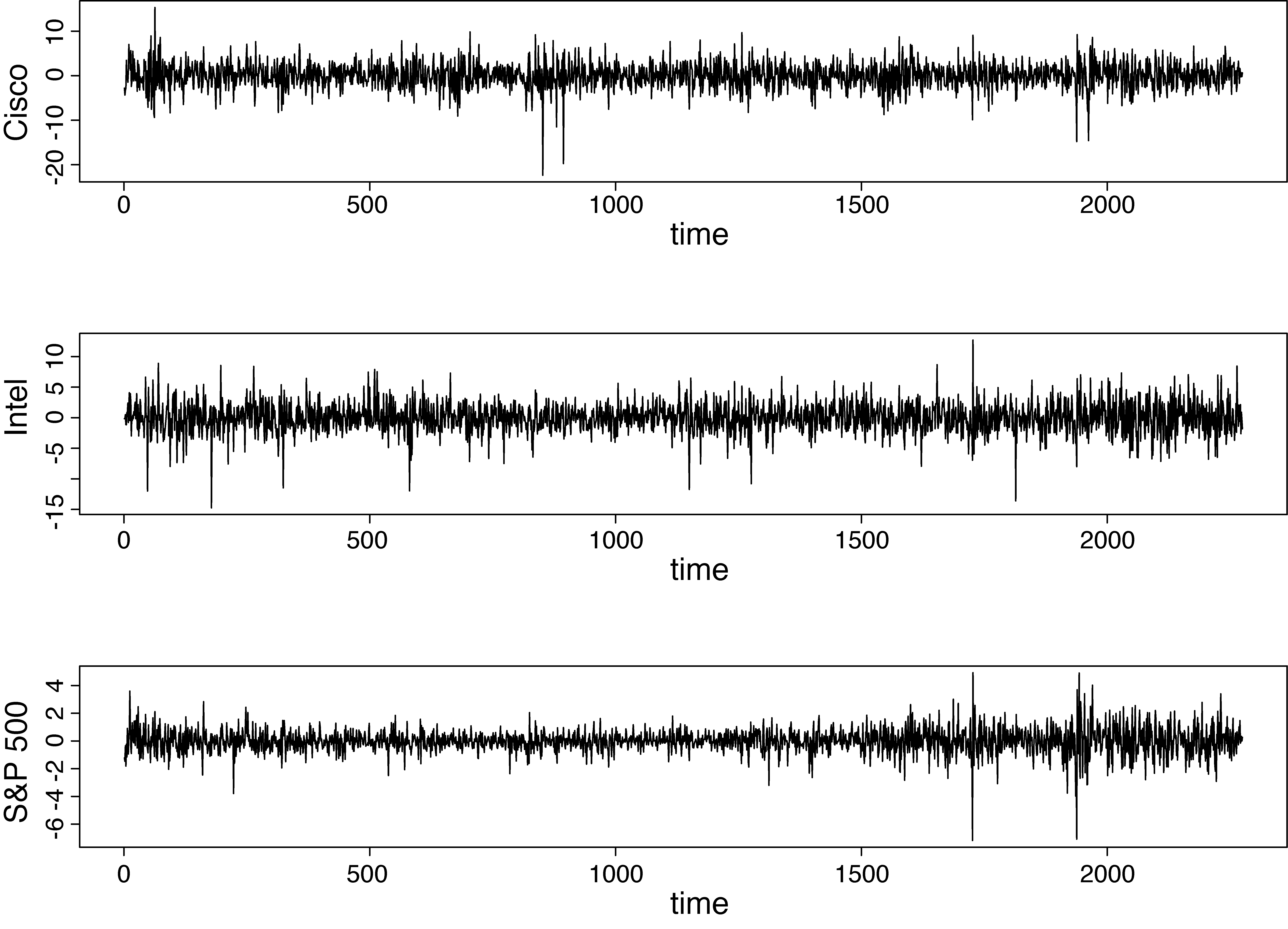
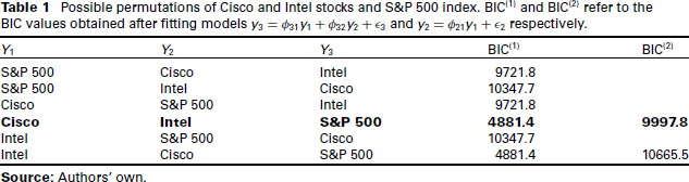
We consider a trivariate series of $n = 2275$ daily log returns of the stocks of Cisco Systems and Intel Corporation, and the S&P 500 index recorded from 2 January 1991 to 31 December 1999. The data have been used for several illustration purposes in Tsay, 2010 and are available online at http://faculty.chicagobooth.[edu/ruey.tsay/teaching/]. The series have been ordered according to the BIC obtained from linear regression models of the form $y_{j} = \sum_{k = 1}^{j - 1} ϕ_{jk} y_{k} + ε_{j}$ , $j = 1, 2, 3$ , as described in Section 3. More specifically, for each of the $3!$ permutations given in Table 1, we fitted the following regression model to the centred values of the series:

y_{3} = ϕ_{31} y_{1} + ϕ_{32} y_{2} + ε_{3} .

(4.1)

Table 1:

Possible permutations of Cisco and Intel stocks and S&P 500 index. BIC $^{(1)}$ and BIC $^{(2)}$ refer to the BIC values obtained after fitting models $y_{3} = ϕ_{31} y_{1} + ϕ_{32} y_{2} + ε_{3}$ and $y_{2} = ϕ_{21} y_{1} + ε_{2}$ respectively.

, $Y_{1}$	$Y_{2}$	$Y_{3}$	BIC $^{(1)}$	BIC $^{(2)}$
S&P 500	Cisco	Intel	$9721.8$
S&P 500	Intel	Cisco	$10347.7$
Cisco	S&P 500	Intel	$9721.8$
Cisco	Intel	S&P 500	$4881.4$	$9997.8$
Intel	S&P 500	Cisco	$10347.7$
Intel	Cisco	S&P 500	$4881.4$	$10665.5$

Authors’ own.

Figure 3:

Authors’ own.

As $Y_{3}$ was selected the S&P 500 index series, i.e., the variable that produced the lower BIC after fitting model (4.1). Having selected $Y_{3}$ , we fitted a model of the form $y_{2} = ϕ_{21} y_{1} + ε_{2}$ to the centred values of the remaining two variables in turn. Hence the candidate models were $Intel = ϕ_{21} Cisco + ε_{2}$ and $Cisco = ϕ_{21} Intel + ε_{2}$ . Again, based on BIC we selected the Intel and Cisco stock series as $Y_{2}$ and $Y_{1}$ respectively. The selected order of the stocks according to this process is indicated in Table 1 by boldface. Hence, we denote the daily log returns of Cisco and Intel stocks and the S&P 500 index by $y_{1; t}, y_{2; t}$ and $y_{3; t}$ respectively. Figures 1 and 2 include the time series plot of $y_{t}$ and their scatterplots. 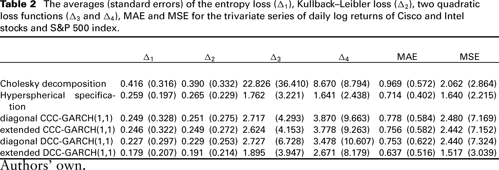The three series are significantly correlated with $corr (y_{1}, y_{2}) = 0.47$ , $corr (y_{1}, y_{3}) = 0.52$ and $corr (y_{2}, y_{3}) = 0.50$ .

Table 2:

The averages (standard errors) of the entropy loss ( $Δ_{1}$ ), Kullback–Leibler loss ( $Δ_{2}$ ), two quadratic loss functions ( $Δ_{3}$ and $Δ_{4}$ ), MAE and MSE for the trivariate series of daily log returns of Cisco and Intel stocks and S&P 500 index.

,
	$Δ_{1}$		$Δ_{2}$		$Δ_{3}$		$Δ_{4}$		MAE		MSE

Cholesky decomposition	$0.416$	$(0.316)$	$0.390$	$(0.332)$	$22.826$	$(36.410)$	$8.670$	$(8.794)$	$0.969$	$(0.572)$	$2.062$	( $2.864$ )
Hyperspherical specification	$0.259$	$(0.197)$	$0.265$	$(0.229)$	$1.762$	$(3.221)$	$1.641$	$(2.438)$	$0.714$	( $0.402$ )	$1.640$	( $2.215$ )
diagonal CCC-GARCH(1,1)	$0.249$	$(0.328)$	$0.251$	$(0.275)$	$2.717$	$(4.293)$	$3.870$	$(9.663)$	$0.778$	( $0.584$ )	$2.480$	( $7.169$ )
extended CCC-GARCH(1,1)	$0.246$	$(0.322)$	$0.249$	$(0.272)$	$2.624$	$(4.153)$	$3.778$	$(9.263)$	$0.756$	( $0.582$ )	$2.442$	( $7.152$ )
diagonal DCC-GARCH(1,1)	$0.227$	$(0.297)$	$0.229$	$(0.253)$	$2.727$	$(6.728)$	$3.478$	$(10.607)$	$0.753$	( $0.622$ )	$2.440$	( $7.324$ )
extended DCC-GARCH(1,1)	$0.179$	$(0.207)$	$0.191$	$(0.214)$	$1.895$	$(3.947)$	$2.671$	$(8.179)$	$0.637$	( $0.516$ )	$1.517$	( $3.039$ )

Authors’ own.

The appropriateness of log-GARCH(1,1) for modelling the elements of the matrices $D_{t}$ (Cholesky decomposition approach) and $H_{t}$ (hyperspherical specification approach) was assessed by plotting the crude estimates, $log {\tilde{d}}_{j; t}^{2}$ and $log {\tilde{σ}}_{j; t}^{2}$ , versus their lagged-one values, $log {\tilde{d}}_{j; t - 1}^{2}$ and $log {\tilde{σ}}_{j; t - 1}^{2}$ , respectively. The appearance of the linear associations in Figures 3 and 4 indicate that modelling $log d_{j; t}^{2}$ and $log σ_{j; t}^{2}$ through log-GARCH(1,1) models is a reasonable choice.

Figure 4:

Authors’ own.

Table 2 summarizes the results of comparing the performance of different methods. In addition to our proposed methods, we consider CCC- and DCC-GARCH(1,1) models with zero (diagonal) and non-zero (extended) off-diagonal entries in the parameter matrices of the GARCH equation. The extended DCC-GARCH model outperforms all methods in terms of all measures of accuracy, except $Δ_{3}$ and $Δ_{4}$ that suggest the superiority of the hyperspherical specification approach. Comparing our two proposed approaches to each other, the one based on hyperspherical parameterization of the correlation matrix outperforms that based on the Cholesky decomposition according to all criteria. The effectiveness of the alternative models in terms of incorporating the conditional heteroskedasticity feature of the series is illustrated in Figure 5 with all models having similar fit.

Figure 5:

Authors’ own.

4.2 Monthly stock returns of 12 US bluechips

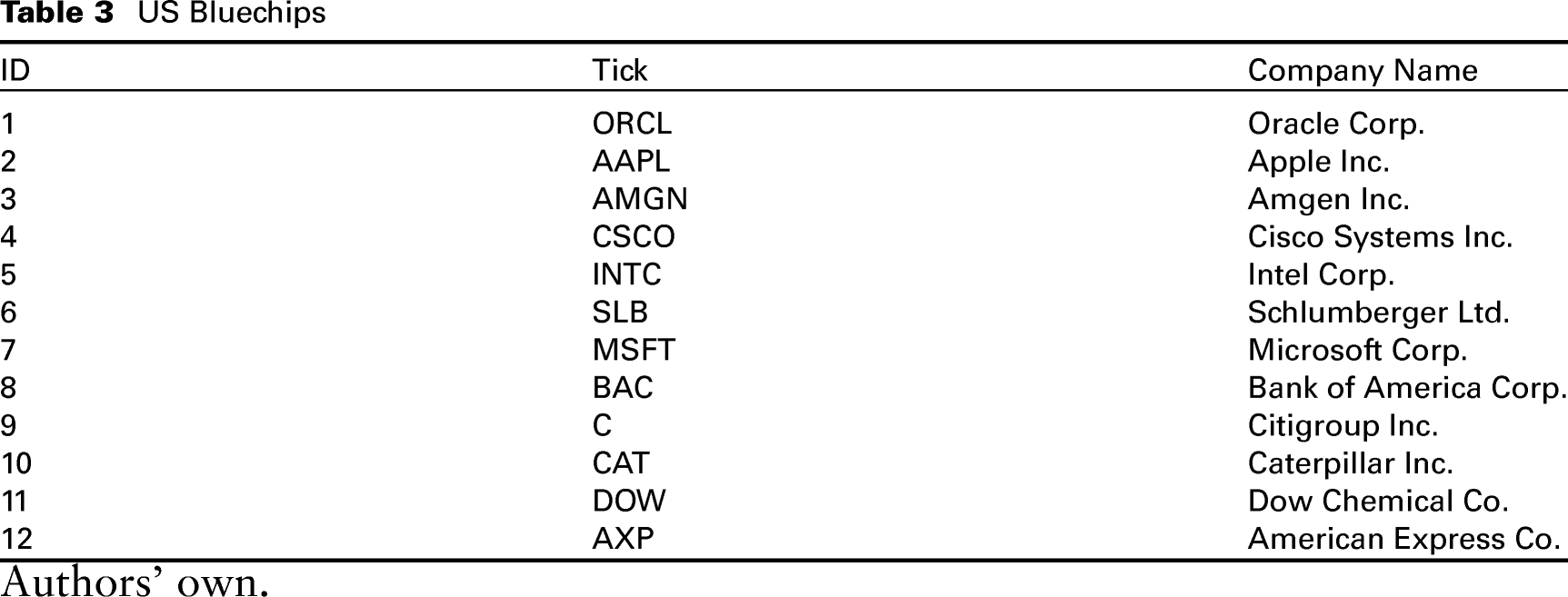
To illustrate the flexibility of the suggested methodology in terms of ease of implementation, we consider compound monthly returns from a panel of 12 US bluechips. The company names are summarized in Table 3 where the stocks are ordered according to the BIC described in Sections 3 and 4.1. The $n = 251$ stock returns were collected from January 1990 to December 2010. For practical purposes, all observations have been multiplied by 10.

Table 3:
US Bluechips

,ID Tick Company Name

1 ORCL Oracle Corp.

2 AAPL Apple Inc.

3 AMGN Amgen Inc.

4 CSCO Cisco Systems Inc.

5 INTC Intel Corp.

6 SLB Schlumberger Ltd.

7 MSFT Microsoft Corp.

8 BAC Bank of America Corp.

9 C Citigroup Inc.

10 CAT Caterpillar Inc.

11 DOW Dow Chemical Co.

12 AXP American Express Co.

,ID	Tick	Company Name
1	ORCL	Oracle Corp.
2	AAPL	Apple Inc.
3	AMGN	Amgen Inc.
4	CSCO	Cisco Systems Inc.
5	INTC	Intel Corp.
6	SLB	Schlumberger Ltd.
7	MSFT	Microsoft Corp.
8	BAC	Bank of America Corp.
9	C	Citigroup Inc.
10	CAT	Caterpillar Inc.
11	DOW	Dow Chemical Co.
12	AXP	American Express Co.

Authors’ own.

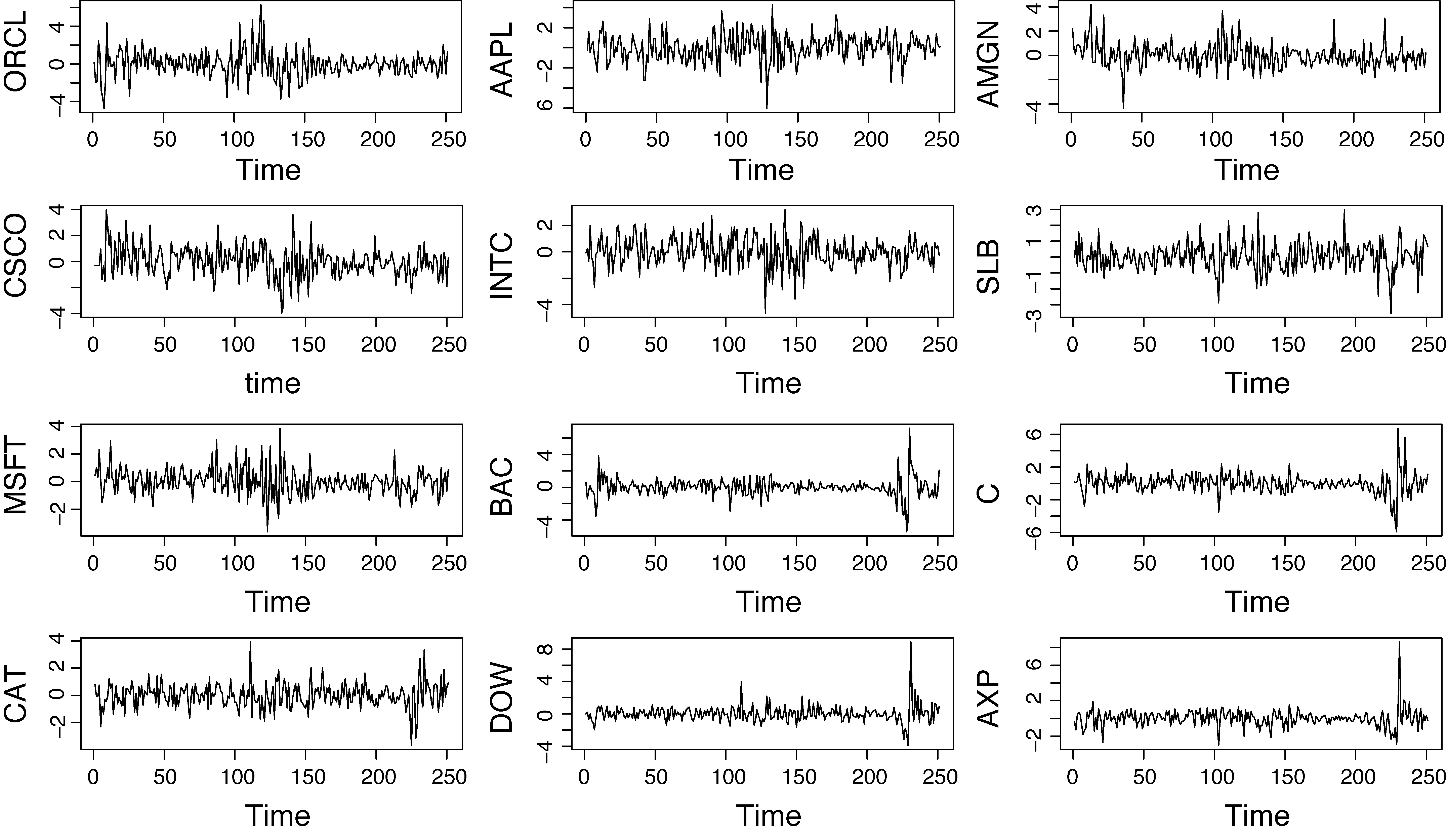
The time series plots and pairwise scatterplots of the 12 series are shown in Figures 6 and 7 respectively. The BAC, C, DOW and AXP stock returns appear less volatile than the other bluechips, whilst cross-correlation rises up to 0.761 (BAC–C).

Table 4:

The averages (standard errors) of the entropy loss ( $Δ_{1}$ ), Kullback–Leibler loss ( $Δ_{2}$ ), the two quadratic loss functions ( $Δ_{3}$ and $Δ_{4}$ ), MAE and MSE for the multivariate series of monthly returns of 12 US bluechips.

,
	$Δ_{1}$		$Δ_{2}$		$Δ_{3}$		$Δ_{4}$		MAE		MSE
Cholesky decomposition	$35.6$	$(17.0)$	$18.6$	$(8.8)$	$106.7$	$(133.0)$	$41.1$	$(49.6)$	$1.002$	( $0.358$ )	$2.440$	( $1.442$ )
Hyperspherical specification	$11.1$	$(5.6)$	$4.9$	$(2.6)$	$3.9$	$(5.3)$	$0.7$	$(2.2)$	$0.321$	( $0.132$ )	$0.242$	( $0.285$ )
diagonal CCC-GARCH(1,1)	$6.9$	$(5.1)$	$4.6$	$(4.2)$	$1.0$	$(1.6)$	$1.6$	$(5.7)$	$0.263$	( $0.190$ )	$0.275$	( $0.634$ )
diagonal DCC-GARCH(1,1)	$7.7$	$(5.9)$	$4.9$	$(4.2)$	$1.1$	$(1.8)$	$1.9$	$(6.6)$	$0.272$	( $0.198$ )	$0.365$	( $1.128$ )

Authors’ own.

Figure 6:

Authors’ own.

Figure 7:

Authors’ own.

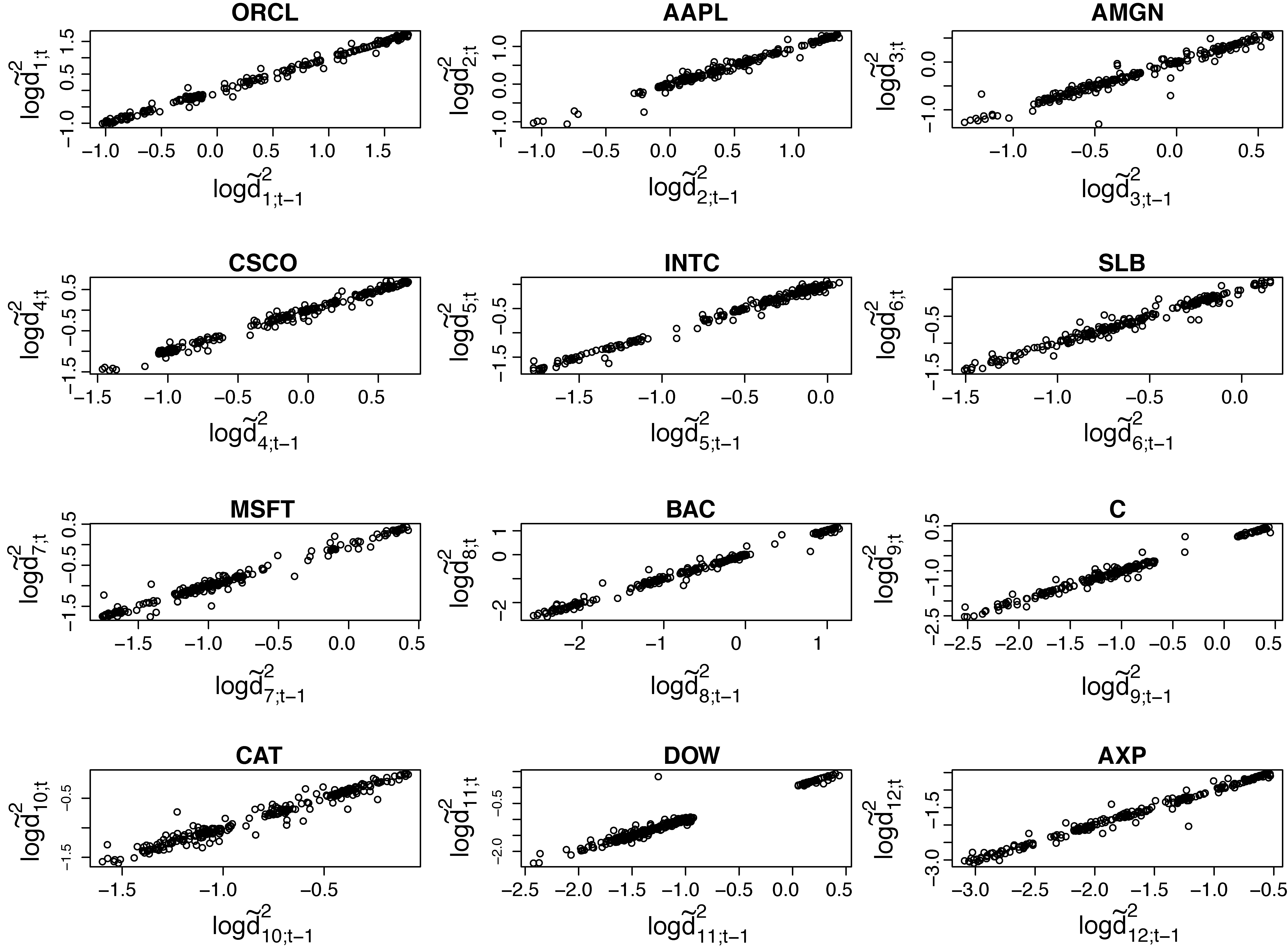
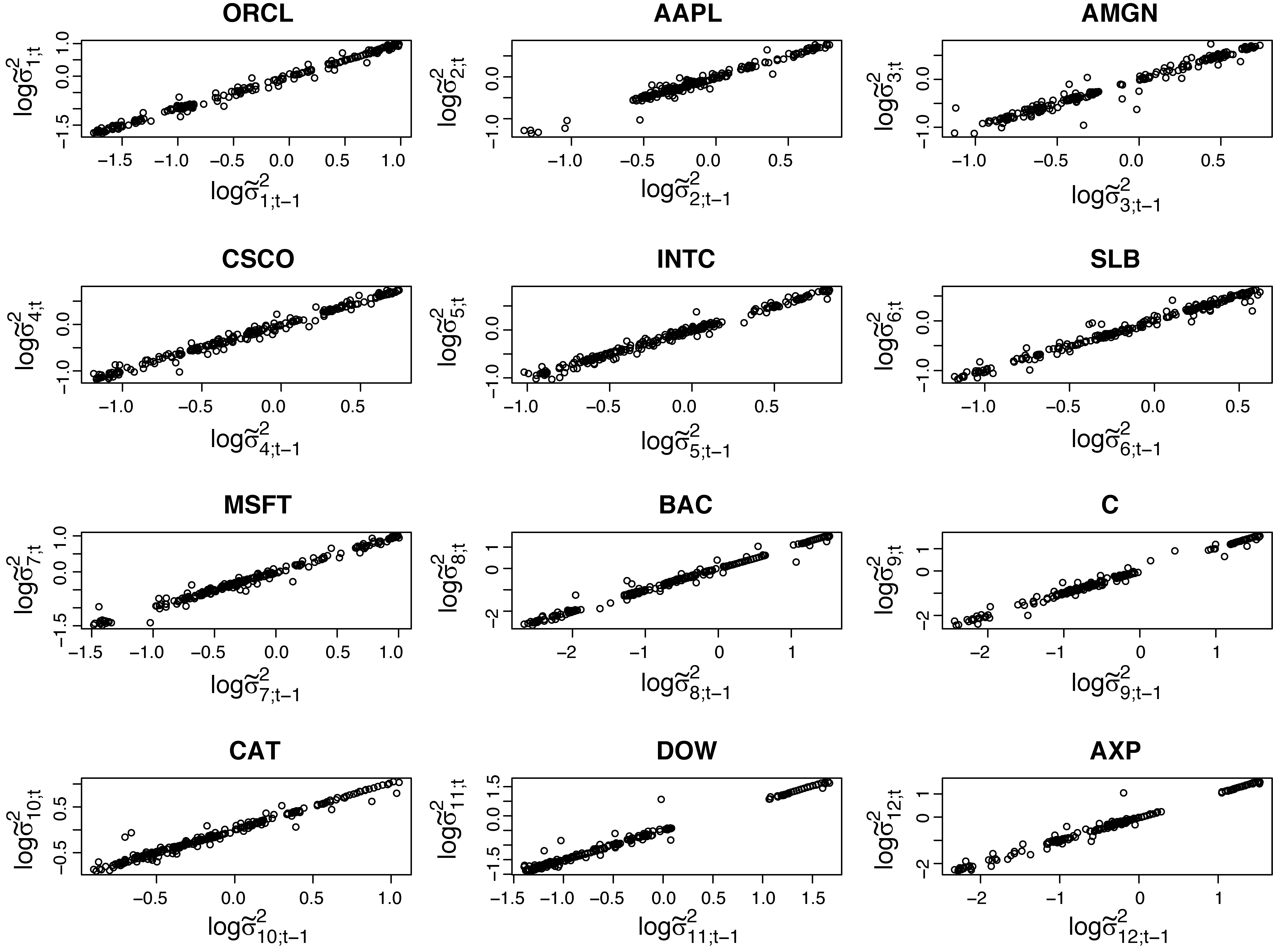
The extended CCC- and DCC-GARCH models considered previously, are now excluded due to convergence problems caused by the large dimension. Regarding the suggested methodology, Figures 8 and 9 provide empirical evidence for the appropriateness of the log-GARCH model for the elements of $D_{t}$ and $H_{t}$ . Results in terms of the accuracy measures $Δ_{1} - Δ_{4}$ , MAE and MSE are summarized in Table 4. Criteria $Δ_{1} - Δ_{3}$ , as well as MAE, support the outperformance of the CCC-GARCH model for this specific dataset. However, the lower variances of $Δ_{2}$ and MAE when calculated under the hyperspherical specification model, indicate that this is probably a more appropriate approach. Such a perspective is also implied by $Δ_{4}$ and MSE. The performance of the Cholesky decomposition approach is inferior when compared to all other models.

Figure 8:

Authors’ own.

Figure 9:

Authors’ own.

Figure 10 displays inference for $σ_{j; t}^{2}$ , $j = 1, \dots, 12$ . Due to space limitation, we omit a similar plot for the covariances $σ_{jk; t}$ , $j = 2, \dots, m$ , $k = 1, \dots, m - 1$ , $k \neq j$ . Overall, patterns similar to those of Figure 6 can be observed in all plots. However, it is interesting to note that each of the series under consideration has special features that are better captured by different models. For instance, whilst the CCC- and DCC-GARCH models are successful in accounting for the peaks observed at the end of the BAC, C, DOW and AXP series, the DCC model obviously fails to capture the variability of the CISCO series. The CCC model and the hyperspherical specification approach seem to perform consistenly better.

Figure 10:

Authors’ own.

In conclusion, our numerical results can be considered as an early indication that the the two methodologies are promising in parsimoniously modelling multivariate volatilities. However, we feel it is important to emphasize that there is no gold standard approach. Actually, one has often to choose between parsimony and ease of implementation versus higher flexibility, and what determines such a decision is based on the data and objectives of a study.

5 Discussion

We considered the modified Cholesky decomposition of a covariance matrix itself, and the standard Cholesky factor of its correlation matrix with hyperspherical reparametrization. The latter leaves the volatilities of the individual assets intact and relies on univariate log-GARCH models for the estimation of time-varying volatilities. The results obtained from the two real data examples and using rather simple models indicate the superior performance of the methodology based on the standard Cholesky decomposition of the correlation matrices and their hyperspherial parameterization. It appears the performance of both models can be improved considerably by the selection of appropriate models and this will be the focus of our future research. When more complicated models are considered, parsimony can be gained by penalizing methods as for instance the lasso regression (Tibshirani, 1996).

Footnotes

Acknowledgments

K. Fokianos and X. Pedeli are supported by a Leventis Foundation grant. M. Pourahmadi is supported by NSF grant DMS-1309586. The authors would like to thank Christian Francq for kindly providing part of the algorithm for the estimation of the log-GARCH model. This work has been carried out while the first author was with the Department of Mathematics and Statistics, University of Cyprus. She would like to thank all the members of the Department for their warm hospitality. Thanks are due to two reviewers and the Associate Editor for their constructive comments.

References

Alexander

(2001) Market models: A guide to financial data analysis . New York: John Wiley.

Bollerslev

(1986) Generalized autoregressive conditional heteroskedasticity. Journal of Econometrics, 31, 307–27.

Bollerslev

(1990) Modelling the coherence in short–run nominal exchange rates: a multivariate generalized arch approach. Review of Economics and Statistics, 72, 498–505.

Bollerslev

Engle

Wooldridge

(1988) A capital asset pricing model with time-varying covariances. The Journal of Political Economy, 96, 116–31.

Chang

Tsay

(2010) Estimation of covariance matrix via the sparse Cholesky factor with lasso. Journal of Statistical Planning and Inference, 140, 3858–73.

Creal

Koopman

Lucas

(2011) A dynamic multivariate heavy-tailed model for time-varying volatilities and correlations. Journal of Business & Economic Statistics, 29, 552–63.

Dellaportas

Pourahmadi

(2004) Large time-varying covariance matrices with applications to finance. Technical Report, Athens University of Economics, Department of Statistics .

Dellaportas

Pourahmadi

(2012) Cholesky–GARCH models with applications to finance. Statistics and Computing, 22, 849–55.

Engle

(1982) Autoregressive conditional heterskedasticity with estimates of the variance of U.K. inflation. Econometrica, 50, 987–1008.

10.

Engle

(2002) Dynamic conditional correlation: a simple class of multivariate generalized autoregressive conditional heteroskedasticity models. Journal of Business amd Economic Statistics, 20, 339–50.

11.

Engle

Kroner

(1995) Multivariate simultaneous generalized ARCH. Econometric Theory, 11, 122–50.

12.

Engle

Rothschild

(1990) Asset pricing with a factor ARCH covariance structure. Journal of Econometrics, 45, 213–38.

13.

Francq

Wintenberger

Zakoian

(2013) GARCH models without positivity constraints: exponential or log GARCH? Journal of Econometrics, 177, 34–46.

14.

Francq

Zakoian

(2010) GARCH models: structure, statistical inference and financial applications. New York: John Wiley.

15.

Geweke

(1986) Modelling the persistence of conditional variances: a comment. Econometric Review, 5, 57–61.

16.

Leng

Zhang

Pan

(2010) Semiparametric mean-covariance regression analysis for longitudinal data. Journal of the American Statistical Association, 105, 181–93.

17.

Lin

Ying

(2001) Semiparametric and nonparametric regression analysis of longitudinal data (with discussions). Journal of the American Statistical Association, 96, 103–26.

18.

Lopes

McCullogh

Tsay

(2012) Cholesky stochastic volatility models for high-dimensional time series. Technical Report, University of Chicago, Booth Business School .

19.

Pan

MacKenzie

(2003) On modelling mean-covariance structures in longitudinal studies. Biometrika, 90, 239–44.

20.

Pan

(2009) Nonparametric regression of covariance structures in longitudinal studies. MIMS Preprint .

21.

Pourahmadi

(1999) Joint mean–covariance models with applications to longitudinal data: Unconstrained parameterization. Biometrika, 86, 677–90.

22.

Pourahmadi

(2000) Maximum likelihood estimation of generalized linear models for multivariate normal covariance matrix. Biometrika, 87, 425–35.

23.

Pourahmadi

(2011) Covariance estimation: The GLM and regularization perspectives. Statistical Science, 26, 369–87.

24.

Rapisarda

Brigo

Mercurio

(2007) Parameterizing correlations: a geometric interpretation. IMA Journal of Management Mathematics, 18, 55–73.

25.

Rebonato

Jäckel

(2000) The most general methodology for creating a valid correlation matrix for risk management and option pricing purposes. Journal of Risk, 2, 17–27.

26.

Silvennoinen

Teräsvirta

(2009) Multivariate garch models. In Mikosch

Kreiß

J-P

Davis

Andersen

(Eds), Handbook of financial time series . Heidelberg, Berlin: Springer, pp. 201–29.

27.

Tibshirani

(1996) Regression shrinkage and selection via the lasso. Journal of the Royal Statistical Society, Series B, 58, 267–88.

28.

Tsay

(2010) Analysis of financial time series (Third Edition) . New York: John Wiley.

29.

Tse

Tsui

(2002) A multivariate generalized autoregressive conditional heteroskedasticity model with time-varying correlations. Journal of Business and Economic Statistics, 20, 351–62.

30.

Vrontos

Dellaportas

Politis

(2003) A full-factor multivariate GARCH model. Econometrics Journal, 52, 2632–49.

31.

Zhang

Leng

Tang

(2014) A joint modelling approach for longitudinal studies. Journal of the Royal Statistical Society: Series B (Statistical Methodology) (to appear) .