The Altham–Poisson distribution

Abstract

The multiplicative binomial model was introduced as a generalization of the binomial distribution for modelling correlated binomial data. This distribution has not been extensively explored and is revisited in the present study. Some properties of the multiplicative binomial distribution, such as, expressions for the factorial moments and the information matrix, are investigated. The distribution is also extended to accommodate data arising from a Wadley's problem setting which is frequently encountered in dose–mortality studies and is one in which the number of organisms initially treated with a drug is unobserved. The Altham–Poisson distribution is introduced by modelling the unobserved initial number of organisms, as specified by $n$ in the multiplicative binomial model, with a Poisson distribution and its suitability for overdispersed data from a Wadley's problem setting is explored.

Keywords

dose–response Multiplicative binomial overdispersion Wadley's problem

1 Introduction

Data generated from a binomial experiment often exhibit over- or underdispersion (Collett, 2003). A number of approaches to the modelling of such data have been proposed. In particular models have been developed in order to accommodate explicitly what are thought to be the underlying causes of the over- and underdispersion. Thus it may well be that there is heterogeneity in the population of interest and that as a consequence the probability of a success is not constant across individuals. Such heterogeneity can lead to overdispersion and is well modelled by allowing the probability of success to follow a beta distribution thereby leading to the beta-binomial distribution (Skellam, 1948; Williams, 1975). It is also possible that deviations in the variance of the data from that of the binomial distribution are related to correlations between individual responses. Such correlations can be modelled explicitly. As an example, Altham (1978) derived the multiplicative binomial distribution for modelling over- and underdispersion by considering a binomial-type experiment in which the binary outcomes have a symmetric joint distribution and are therefore correlated.

Wadley's problem is the main focus of the present study and relates to a binomial experiment in which the number of successes is recorded but the number of trials involved is unknown (Morgan, 1992; Leask, 2009). Wadley (1949) modelled the data generated from such an experiment by taking the unknown number of trials to follow a Poisson distribution and, in a separate study, Anscombe (1949) proposed that overdispersion in the data be accommodated by placing a negative binomial distribution on that unknown number. The question then immediately arises as to whether over- or underdispersion in data generated in a Wadley's problem setting should rather be attributed to deviations from the variance in the underlying binomial distribution. Leask and Haines (2014) addressed this issue by placing a Poisson distribution on the number of trials in the beta-binomial model, thereby accommodating heterogeneity in the underlying population. In the present study, and as a counterpoint to the work of Leask and Haines (2014), emphasis is placed on correlations between individual binary responses. Specifically, the multiplicative binomial distribution developed by Altham (1978) is embedded in Wadley's problem by placing a Poisson distribution on the unknown number of trials in the experiment. The resultant distribution is termed the Altham–Poisson distribution and is developed in order to accommodate both over- and underdispersion in the data.

The paper is structured as follows. The use of the multiplicative binomial distribution as a model for count data and for dose–response data is revisited and critically reviewed in Section 2. The discussion in this section mirrors, but provides a counterpoint to, the results of Altham (1978) and, more recently, Feirer et al. (2013). The Altham–Poisson distribution is then introduced and explored in Section 3 and concluding remarks are presented in Section 4.

2 Multiplicative binomial model

2.1 Probability distribution

The probability mass function (p.m.f.) of the multiplicative binomial distribution was derived by Altham (1978) who considered modelling over- and underdispersed binomial-type data by allowing for first order correlations among binary responses. Consider a random variable $Y$ which represents the number of successes in $n$ trials and suppose that $p$ is the probability of a success, $q = 1 - p$ and that $θ$ is an attenuating parameter. Then the p.m.f. of the multiplicative binomial model is written as

Pr (Y = y) = \frac{(\begin{matrix} n \\ y \end{matrix}) p^{y} q^{n - y} θ^{y (n - y)}}{f (p, θ, n)}, y = 0, \dots, n .

(2.1)

The term

f (p, θ, n)

in expression (2.1) is a normalizing constant given by

f (p, θ, n) = \sum_{y = 0}^{n} (\begin{matrix} n \\ y \end{matrix}) p^{y} q^{n - y} θ^{y (n - y)}

with

0 \leq p \leq 1

and

θ > 0

. Of relevance is the fact that the parameter

θ

is related to

n

through its definition (Altham, 1978). When

n

varies it is sensible to model

θ

in terms of

n

with an appropriate function but, since

n

is constant in the present context, this dependency is not made explicit. The p.m.f. in Equation (2.1) is of a similar form to that of a binomial random variable but with the additional parameter

θ

which allows the model to accommodate both over- and underdispersion. The parameter

p

can be identified as the probability of a success when the individual responses are independent and the distribution is strictly binomial (Lovison, 1997). However, the interpretation of the parameter

θ

must be made with some care (Lovison, 1997, 1998). Specifically,

θ

is a cross-product ratio representing pairwise correlations between the binary responses and is not necessarily directly related to over- and underdispersion relative to the binomial distribution. Indeed Lovison (1997, 1998) and Feirer et al. (2013) observe that the multiplicative binomial model can be used for overdispersed data when

θ < 1

and

p

is close to 0.5 or when

θ > 1

and

p

is close to zero or one and for underdispersed data when

θ > 1

and

p

is close to 0.5 or when

θ < 1

and

p

is close to zero or one. These observations are made explicit in the next subsection. Note also that the multiplicative binomial reduces to the binomial distribution when

θ = 1

Lovison (1997, 1998) presented an alternative derivation of the multiplicative binomial distribution to that of Altham (1978) which was based on methods introduced by Cox (1972). In addition Molenberghs and Ryan (1999) derived a distribution to model clustered binary data in developmental toxicity studies identical to the multiplicative binomial distribution by using a technique similar to that of Lovison (1997) but did not identify the connection.

2.2 Statistical properties of the distribution

Some properties of the multiplicative binomial distribution have been explored in the literature. Properties of the model that have not previously been examined or presented are included in this section.

Altham (1978) derived expressions for the first and second factorial moments of the multiplicative binomial distribution. In fact, a more general expression for the factorial moments can be readily derived and is given by

E [Y^{(r)} {(n - Y)}^{(s)}] = n (n - 1) \dots (n - 2 r + 1) p^{r} q^{r} θ^{r (n - r)} \frac{f (p, θ, n - 2 r)}{f (p, θ, n)}

when

r = s

\begin{matrix} E [Y^{(r)} {(n - Y)}^{(s)}] & = & \frac{n (n - 1) \dots (n - s - r + 1) p^{r} q^{s} θ^{r (n - r)} {(p θ^{s - r} + q)}^{n - s - r}}{f (p, θ, n)} \\ \times f (\frac{p θ^{s - r}}{p θ^{s - r} + q}, θ, n - s - r) \end{matrix}

when

s > r

and

\begin{matrix} E [Y^{(r)} {(n - Y)}^{(s)}] & = & \frac{n (n - 1) \dots (n - r - s + 1) p^{r} q^{s} θ^{s (n - y)} {(p + q θ^{r - s})}^{n - s - r}}{f (p, θ, n)} \\ \times f (\frac{p}{p + q θ^{r - s}}, θ, n - r - s) \end{matrix}

when

r > s

. Full details are available in Leask (2009). The factorial moments can be used to obtain the mean, variance, skewness and kurtosis of the multiplicative binomial distribution. Expressions for the mean and variance of the multiplicative binomial distribution have been provided by Altham (1978), while the expressions for the skewness and kurtosis are not algebraically tractable and as a result are not presented here. Note that the probability generating function of the multiplicative binomial distribution is given by

E (s^{Y}) = (ps + q) - n f (\frac{ps}{ps + q}, θ, n) / f (p, θ, n)

and includes a normalizing constant which depends on the indeterminate,

s

. It is therefore easier to obtain expressions for the moments of the multiplicative binomial distribution directly from the factorial moments as defined above.

The mean and the variance of the multiplicative binomial distribution are given succinctly by

E (Y) = np τ_{1} and Var (Y) = np (τ_{1} - τ_{2} p),

where

τ_{1} = \frac{{(p + q θ)}^{n - 1}}{f (p, θ, n)} f (\frac{p}{p + q θ}, θ, n - 1)

and

τ_{2} = n τ_{1}^{2} - \frac{(n - 1) {(p + q θ^{2})}^{n - 2}}{f (p, θ, n)} f (\frac{p}{p + q θ^{2}}, θ, n - 2) .

Thus, the expression for the variance can be used to quantify the relationship between the parameters

θ

and

p

and the over- or underdispersion of the multiplicative binomial relative to the binomial distribution, a relationship which is presented graphically in Figure 8 of the paper by Feirer et al. (2013).

The modality of the multiplicative binomial distribution was investigated by Zelterman (2004) who showed that the distribution is unimodal when $θ > 1$ . It can also be shown that the multiplicative binomial distribution can be either multimodal or unimodal when $θ < 1$ (Leask, 2009).

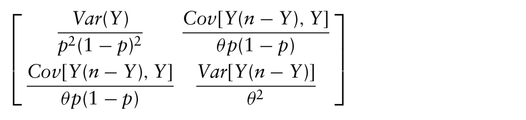
The log-likelihood and score functions of the multiplicative binomial distribution were presented in the paper by Altham (1978). In the present study the information matrix for the parameters $p$ and $θ$ was also derived as

[\begin{matrix} \frac{V a r (Y)}{p^{2} {(1 - p)}^{2}} & \frac{C o v [Y (n - Y), Y]}{θ p (1 - p)} \\ \frac{C o v [Y (n - Y), Y]}{θ p (1 - p)} & \frac{V a r [Y (n - Y)]}{θ^{2}} \end{matrix}]

and can be used to obtain the standard errors of the parameter estimates. Note that the derivation of the information matrix is given in Appendix A.

Böhning et al. (2013) recently re-introduced the notion of a ratio plot (Ord, 1967) as a powerful technique for identifying a suitable distribution with which to model a discrete dataset. The authors provide a number of valuable insights into and extensions of the technique and use the approach within the context of Poisson-based distributions for modelling capture–recapture data. Feirer et al. (2013) refer briefly to the use of ratio plots within the context of the multiplicative binomial and the double binomial distributions but give no details. In such cases, and thus in the present case, the binomial must be regarded as the baseline distribution. Then a scaled ratio of probabilities can be introduced as

r_{y} = \frac{(y + 1)}{(n - y)} \frac{Pr (Y = y + 1)}{Pr (Y = y)}

and is a constant,

\frac{p}{1 - p}

, for the binomial distribution. It is straightforward to show that the ratio for the multiplicative binomial distribution is given by

r_{y} = \frac{p}{1 - p} θ^{n - 1} \frac{1}{θ^{2 y}}

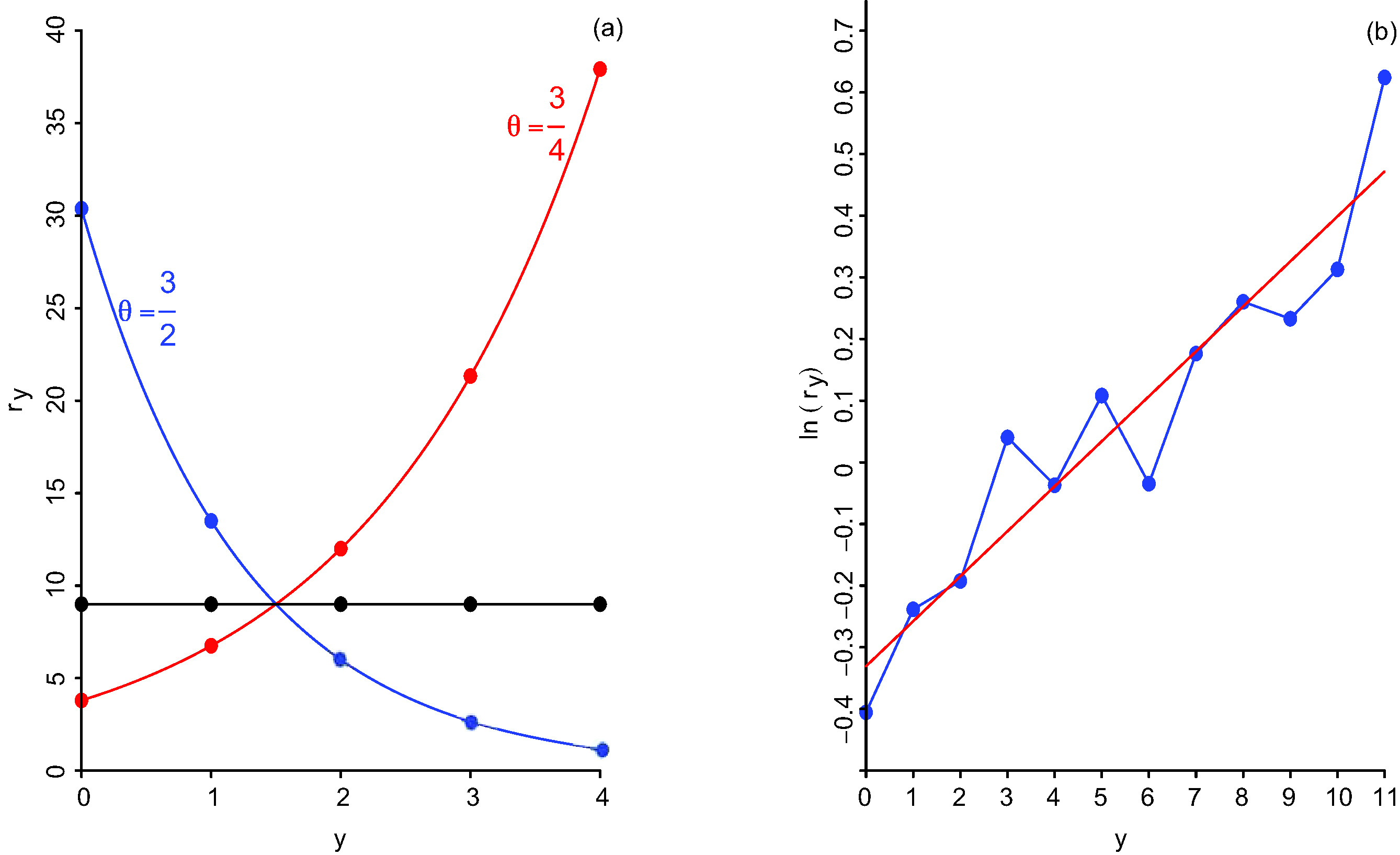
and plots of

r_{y}

against

y

for this distribution with

n = 4

p = 0.9

and

θ = \frac{3}{4}, 1

and

\frac{3}{2}

are shown in Figure 1(a).

Figure 1

Source: Authors' computation.

Clearly

ln (r_{y}) = ln (\frac{p}{1 - p}) + (n - 1) ln (θ) - 2 y ln (θ)

and thus plots of

ln (r_{y})

against

y

are linear with a negative slope if

θ > 1

, with a positive slope if

θ < 1

and represent a constant if

θ = 1

. The following example is now introduced in order to illustrate the use of the ratio plot technique within the context of the multiplicative binomial distribution.

2.3 Example

Lindsey (1995, p. 131) presented data comprising the number of boys born to 6115 families of 13 children, with the last birth not counted (Dataset 1, Appendix C). The data originated from a study by Geissler (see Edwards, 1958) and the analysis has been reported in a number of papers and books on discrete data. Estimates of the ratio $r_{y}$ , denoted as ${\hat{r}}_{y}$ , were obtained by replacing the probabilities embedded in $r_{y}$ by observed frequencies and a plot of $ln ({\hat{r}}_{y})$ against $y$ is shown in Figure 1(b). A straight line was fitted to the points of this plot using ordinary least squares and provided a good fit with an $R^{2}$ value of $89 %$ , an intercept of $- 0.331$ and a slope of $0.0729$ . The results indicate that the multiplicative binomial distribution should give an appropriate fit to the frequency data and, since the slope of the line is positive, that $θ < 1$ . Following Böhning et al. (2013), rough estimates of the parameters $p$ and $θ$ can be calculated from the intercept and slope of the fitted line and are given by $0.490$ and $0.964$ respectively. These estimates can be used as initial values in fitting the multiplicative binomial distribution to the data and indeed are close to the respective maximum likelihood estimates (MLEs) of $0.516$ and $0.974$ . The use of weighted least squares regression in fitting ratio plots, as suggested by Böhning et al. (2013), was not invoked in the present example since suitable weights, inversely proportional to estimates of the variance of $ln ({\hat{r}}_{y})$ , would not seem to be immediately available from the frequency data. Finally note that the MLEs of the mean and variance of the fitted multiplicative binomial distribution are given by $6.231$ and $3.489$ respectively, with the variance indicating extra-binomial dispersion in the data. Note also, as an aside, that the $χ^{2}$ -test statistic is $2.86$ with 10 degrees of freedom indicating that the multiplicative binomial distribution provides an excellent fit to the data.

2.4 Modelling overdispersed dose–response data

Lindsey and Altham (1998) considered using the multiplicative binomial distribution in a dose–response context by modelling $p$ in terms of the explanatory variables with a logit-link function and modelling $θ$ in terms of $n$ with a log-link function. In addition Molenberghs and Ryan (1999) used the multiplicative binomial distribution with $n$ fixed to model data arising from developmental toxicity studies and modelled $p$ as a linear function of the dose administered. Furthermore Feirer et al. (2013) modelled over- and underdispersed printability data using the multiplicative binomial distribution with a logit function to model the parameter $p$ in terms of the explanatory variables and again took $n$ to be fixed. In the present study, a dose–response scenario with a logit-link, natural mortality and a fixed number of observations at each dose is considered.

Suppose that the parameter $λ$ represents the proportion of natural mortality with $0 \leq λ \leq 1$ . Then the parameter $p$ of the multiplicative binomial distribution can be modelled as a function of log-dose $x$ using a logit-link as

p = λ + \frac{1 - λ}{1 + e^{- (α + β x)}},

(2.2)

where

α

and

β

are unknown parameters. Specifically, consider a random variable

Y

that denotes the number of organisms that survive treatment with varying doses of a particular drug. Suppose that

n

experiments are conducted at the

i

th dose

d_{i}

, and thus the log-dose

x_{i} = ln (d_{i})

x_{i} = log (d_{i})

for

i = 1, \dots, D

. Then

y_{ij}

refers to the number of survivors in the

j

th experiment using dose

d_{i}

of the drug for

i = 1, \dots, D

and

j = 1, \dots, n

. Furthermore, let

p_{i}

denote the probability of an organism surviving exposure to the

i

th dose of the drug and consider writing this probability in terms of the log-dose using expression (2.2). Then the likelihood function for the multiplicative binomial model with

p

modelled with the logit-link function can be written as

L (λ, α, β, θ;) = \prod_{i = 1}^{D} \prod_{j = 1}^{n} \frac{(\begin{matrix} n \\ y_{i j} \end{matrix}) p_{i}^{y_{ij}} {(1 - p_{i})}^{n - y_{ij}} θ^{y_{ij} (n - y_{ij})}}{f (p_{i}, θ, n)},

where y represents the vector of observations.

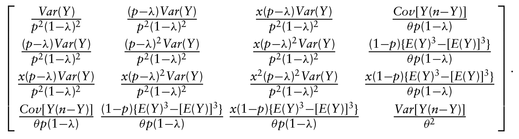
The information matrix presented in Section 2.2 can be adapted for a dose–response setting by considering the relationship between $p$ and the parameters $α, β$ and $λ$ . Thus the information matrix for the parameters and is readily derived as

[\begin{matrix} \frac{Var (Y)}{p^{2} {(1 - λ)}^{2}} & \frac{(p - λ) Var (Y)}{p^{2} {(1 - λ)}^{2}} & \frac{x (p - λ) Var (Y)}{p^{2} {(1 - λ)}^{2}} & \frac{Cov [Y (n - Y)]}{θ p (1 - λ)} \\ \frac{(p - λ) Var (Y)}{p^{2} {(1 - λ)}^{2}} & \frac{{(p - λ)}^{2} Var (Y)}{p^{2} {(1 - λ)}^{2}} & \frac{x {(p - λ)}^{2} Var (Y)}{p^{2} {(1 - λ)}^{2}} & \frac{(1 - p) {E {(Y)}^{3} - {[E (Y)]}^{3}}}{θ p (1 - λ)} \\ \frac{x (p - λ) Var (Y)}{p^{2} {(1 - λ)}^{2}} & \frac{x {(p - λ)}^{2} Var (Y)}{p^{2} {(1 - λ)}^{2}} & \frac{x^{2} {(p - λ)}^{2} Var (Y)}{p^{2} {(1 - λ)}^{2}} & \frac{x (1 - p) {E {(Y)}^{3} - {[E (Y)]}^{3}}}{θ p (1 - λ)} \\ \frac{Cov [Y (n - Y)]}{θ p (1 - λ)} & \frac{(1 - p) {E {(Y)}^{3} - {[E (Y)]}^{3}}}{θ p (1 - λ)} & \frac{x (1 - p) {E {(Y)}^{3} - {[E (Y)]}^{3}}}{θ p (1 - λ)} & \frac{Var [Y (n - Y)]}{θ^{2}} \end{matrix}] .

The parameters $λ, α, β$ and $θ$ of the multiplicative binomial distribution can then be estimated by optimizing the log of the likelihood function directly using a numerical optimization routine. A starting value of 1 can be used for $θ$ and starting values for the parameters $λ, α$ and $β$ can be obtained from fitting a binomial distribution with $p$ modelled with a logit-link function that includes natural mortality as in expression (2.2). The standard errors of the parameter estimates can be obtained from the information matrix in the usual way and 95% Wald intervals thus calculated for each parameter. Profile likelihood plots can also be produced for each parameter and these plots can be used to compute 95% confidence interval estimates. Consider, for example, the confidence interval for the parameter $θ$ . Suppose that $ℓ = ℓ (\hat{λ}, \hat{α}, \hat{β}, \hat{θ};)$ is the maximum log-likelihood of the multiplicative binomial distribution and let $ℓ_{p} (θ)$ denote the profile log-likelihood for the parameter $θ$ . The 95% confidence interval for $θ$ is then given by $[θ_{1}, θ_{2}]$ where $θ_{1}$ and $θ_{2}$ satisfy

ℓ_{p} (θ_{1}) = ℓ_{p} (θ_{2}) = ℓ - \frac{1}{2} χ_{1, 0.05}^{2}

(Azzalini, 1996). Similarly, 95% confidence intervals for

α, β

and

λ

can be obtained by producing profile likelihood plots for these parameters.

The fit of the multiplicative binomial distribution can be assessed in a number of ways. Thus, in order to determine whether the multiplicative binomial would be a more suitable model than the binomial model for a given dataset, the hypothesis $H_{0} : θ = 1$ against $H_{1} : θ \neq 1$ can be tested using the likelihood ratio test (Feirer et al., 2013). Furthermore, plots of Pearson residuals, that is, residuals constructed as the ratio of observed minus fitted values to the appropriate standard errors, against the fitted values can be used to determine whether a model adequately fits the data (Azzalini, 1996). Within the context of model selection, the multiplicative binomial distribution can be compared with other distributions by invoking Akaike's information criterion (AIC), where the model with the lowest AIC value is to be preferred. Ratio plots for dose–response data are not useful, at least in general, since the probability $p$ is related to $y$ through the dose (or log-dose) of the drug administered and as a consequence the data are not necessarily representative of the entire range of $y$ . Ratio plots for dose–response data are therefore not considered in the present study.

2.5 Example

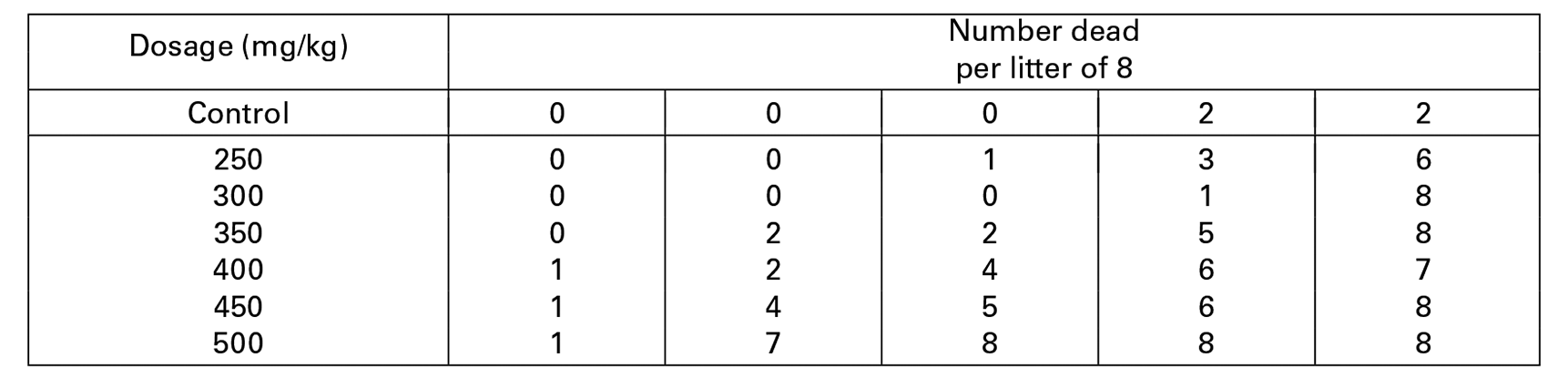
Morgan (1992) presented a dataset in which varying doses of trichloromethane were administered to litters of eight mice seven days after birth and the number that died within 14 days of exposure to the drug was recorded (Dataset 2, Appendix C). Morgan (1992) observed that the variation in the responses exceeds the variation that would be explained by a binomial model and concluded that the data are overdispersed. Since the data are overdispersed, the multiplicative binomial distribution with the probability $p$ modelled by a logit-link function including natural mortality was fitted to Morgan's, (1992) mice data using a direct and straightforward optimization routine. The maximum likelihood estimates of the parameters, together with their standard errors and 95% confidence intervals, are presented in Table 1.

Table 1
Results from fitting the multiplicative binomial model to the mice data, where $p$ is modelled with a logit function and $λ$ is the rate of natural mortality.

Parameter Estimate Std. Error 95% Profile CI 95% Wald CI

$\hat{λ}$ 0.3572 0.0800 $(0; 0.41)$ $(0.20; 0.51)$

$\hat{α}$ $- 14.8232$ 9.7414 $(; - 4.25)$ $(- 33.92; 4.27)$

$\hat{β}$ 5.2287 3.5624 $(1.3; )$ $(- 1.75; 12.21)$

$\hat{θ}$ 0.7231 0.0234 $(0.68; 0.77)$ $(0.68; 0.77)$

Parameter	Estimate	Std. Error	95% Profile CI	95% Wald CI
$\hat{λ}$	0.3572	0.0800	$(0; 0.41)$	$(0.20; 0.51)$
$\hat{α}$	$- 14.8232$	9.7414	$(*; - 4.25)$	$(- 33.92; 4.27)$
$\hat{β}$	5.2287	3.5624	$(1.3; *)$	$(- 1.75; 12.21)$
$\hat{θ}$	0.7231	0.0234	$(0.68; 0.77)$	$(0.68; 0.77)$

Source: Authors' computation.

Note: * These limits of the confidence intervals cannot be computed.

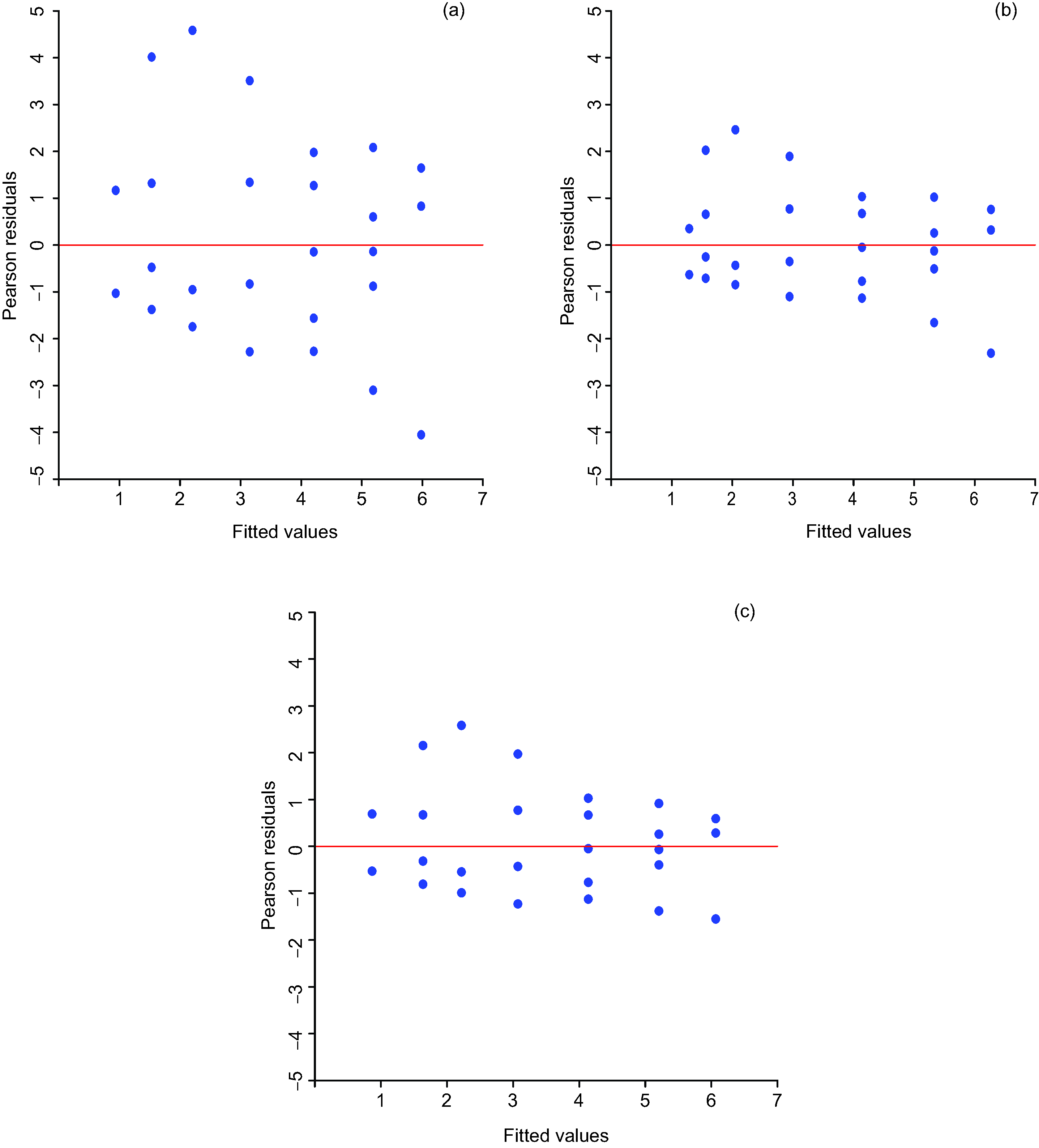
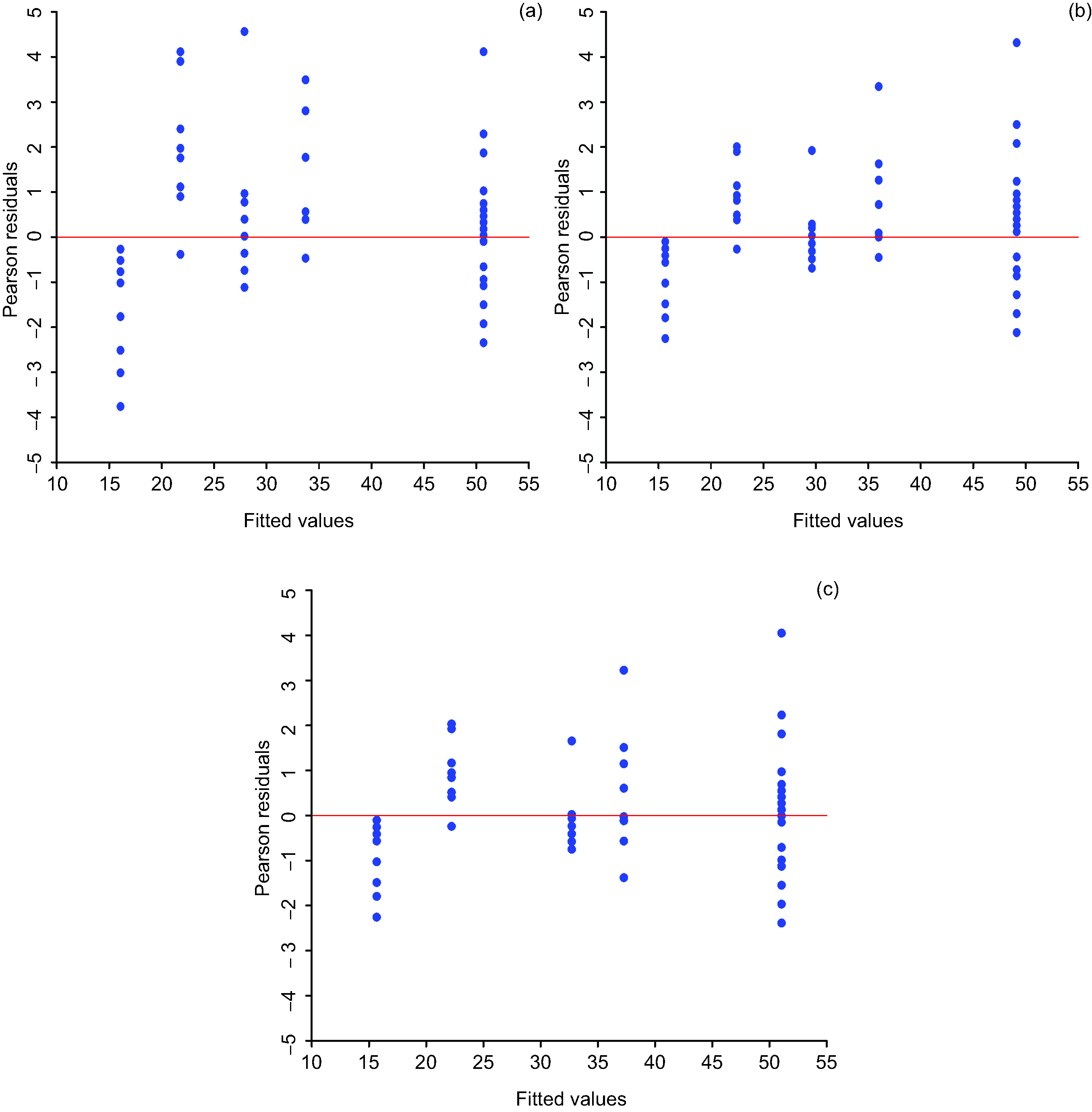
In order to determine whether a multiplicative binomial would be more suitable than the binomial model, the two-sided hypothesis $H_{0} : θ = 1$ against $H_{1} : θ \neq 1$ was tested. The value of the Wald test statistic for this hypothesis was 140.03 which, when compared with a $χ_{1}^{2}$ distribution, yielded a p-value less than 0.0001 indicating that the multiplicative binomial model provides a better fit to this dataset than the binomial. This conclusion is supported by the plots of Pearson residuals against fitted values for the binomial and the multiplicative binomial models shown in Figures 2(a) and 2(c) respectively. The residual plot for the beta-binomial, which is shown in Figure 2(b), is comparable with that for the multiplicative binomial model. However, the AIC values, presented in Table 2, indicate that the multiplicative binomial model is to be preferred.

Figure 2

Source: Authors' computation.

Table 2

A comparison of the models fitted to the mice data.

Model	Maximuma log-likelihood	Number of parameters	AIC
Multiplicative binomial	−64.90	4	137.80
Beta-binomial	−126.43	4	260.86
Binomial	−160.15	3	326.30

Source: Authors' computation.

3 Altham–Poisson distribution

3.1 Derivation of the p.m.f.

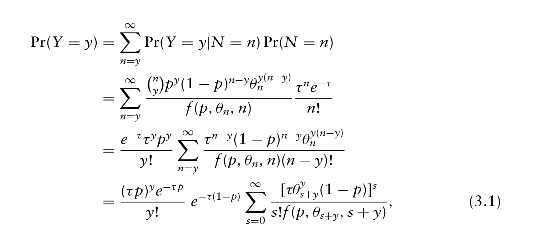
Consider a random variable $Y$ which follows a multiplicative binomial distribution with the number of trials $n$ and parameters $p$ and $θ$ . Suppose that the number of trials is unobserved and, in accordance with Wadley (1949), consider modelling this unknown number as a random variable $N$ with a Poisson( $τ$ ) distribution. Using the notation introduced in Section 2, let $f (p, θ, n)$ denote the normalizing constant of the multiplicative binomial distribution. Then the p.m.f. of the Altham–Poisson distribution is that of a weighted Poisson model and is given by

\begin{matrix} Pr (Y = y) & = & \sum_{n = y}^{\infty} Pr (Y = y | N = n) Pr (N = n) \\ = & \sum_{n = y}^{\infty} \frac{(\begin{matrix} n \\ y \end{matrix}) p^{y} {(1 - p)}^{n - y} θ_{n}^{y (n - y)}}{f (p, θ_{n}, n)} \frac{τ^{n} e^{- τ}}{n!} \\ = & \frac{e^{- τ} τ^{y} p^{y}}{y!} \sum_{n = y}^{\infty} \frac{τ^{n - y} {(1 - p)}^{n - y} θ_{n}^{y (n - y)}}{f (p, θ_{n}, n) (n - y)!} \\ = & \frac{{(τ p)}^{y} e^{- τ p}}{y!} e^{- τ (1 - p)} \sum_{s = 0}^{\infty} \frac{{[τ θ_{s + y}^{y} (1 - p)]}^{s}}{s! f (p, θ_{s + y}, s + y)}, \end{matrix}

(3.1)

where the parameter

θ

must now necessarily be modelled as a function of

n

and is denoted as

θ_{n}

The distribution of $Y$ will be referred to as the Altham–Poisson distribution with parameters $τ$ and $p$ together with the parameters embedded in the model for $θ_{n}$ . The p.m.f. in expression (3.1) indicates that evaluating a probability for the Altham–Poisson distribution entails the approximation of an infinite sum and it is desirable to approximate the infinite sum to a specified degree of accuracy. It can be shown that this infinite sum is bounded above (see Appendix B for details) and as a result the sum can be approximated by a finite sum for which the accuracy of the approximation can be controlled.

3.2 Statistical properties of the distribution

Since the p.m.f. of the random variable $Y$ includes an infinite sum, the moments of the Altham–Poisson distribution cannot be written down in closed form. In particular, expressions for the moments of the Altham–Poisson distribution include an infinite sum within an infinite sum. The first two moments are presented here. If $Y$ follows an Altham–Poisson distribution with parameters $τ, p$ and those embedded in $θ_{n}$ then the expected values of $Y$ and $Y^{2}$ are written as

E (Y) = \sum_{y = 0}^{\infty} y \frac{{(τ p)}^{y} e^{- τ}}{y!} \sum_{s = 0}^{\infty} \frac{{[τ θ_{s + y}^{y} (1 - p)]}^{s}}{s! f (p, θ_{s + y}, s + y)}

and

E (Y^{2}) = \sum_{y = 0}^{\infty} y^{2} \frac{{(τ p)}^{y} e^{- τ}}{y!} \sum_{s = 0}^{\infty} \frac{{[τ θ_{s + y}^{y} (1 - p)]}^{s}}{s! f (p, θ_{s + y}, s + y)},

respectively.

Three techniques for approximating these moments with a specified model for the parameter $θ_{n}$ may be employed. Specifically, the first two factorial moments, and hence the mean and variance, of the Altham–Poisson distribution can be estimated using finite expressions in place of the infinite sums embedded in $E (Y)$ and $E (Y^{2})$ by selecting suitable cutoff values for $y$ and $s$ . Determining these cutoff values, however, is not trivial and therefore other methods are considered. Thus another method entails simulating a large number of observations from the Altham–Poisson distribution by first simulating a value of $N$ from the Poisson( $τ$ ) distribution and then a value of $Y$ given $N = n$ from the multiplicative binomial distribution with parameters $p$ and $θ_{n}$ . The mean and variance of the simulated observations then provide estimates of the mean and variance of the Altham–Poisson distribution with parameters $τ, p$ and $θ_{n}$ . However, this approach is computationally demanding since a large number of simulated observations are required in order to achieve a reasonable accuracy for the moments. An alternative, and more preferable, method of approximating the moments of the Altham–Poisson distribution is to condition on the distribution of $N$ in the following way:

\begin{matrix} E (Y) & = & E_{N} [E (Y | N = n)] \\ = & E_{N} [np {(p + q θ_{n})}^{n - 1} f (\frac{p}{p + q}, θ_{n}, n - 1) / f (p, θ_{n}, n)] \end{matrix}

and

\begin{matrix} E [Y (Y - 1)] & = & E_{N} {E [Y (Y - 1) | N = n]} \\ = & E_{N} [n (n - 1) p^{2} {(p + q θ_{n}^{2})}^{n - 2} f (\frac{p}{p + q^{2}}, θ_{n}, n - 2) / f (p, θ_{n}, n)], \end{matrix}

where

E [Y | N = n]

and

E [Y (Y - 1) | N = n]

are the expectations of a random variable following a multiplicative binomial distribution from Section 2. The moments can then be estimated by simulating values of

n

from a Poisson distribution with parameter

τ

and computing the expected values of

Y

and

Y (Y - 1)

for each value of

n

using the relevant moments from the multiplicative binomial distribution. The averages of these expectations then provide estimates of the required moments. This approach is not computationally demanding in terms of numbers of simulations and is to be preferred.

The ratio plot for the Altham–Poisson distribution is determined, following Böhning et al. (2013), by the ratio

r_{y} = \frac{(y + 1) Pr (Y = y + 1)}{Pr (Y = y)} = τ p \frac{S_{y + 1}}{S_{y}},

where

S_{y} = \sum_{s = 0}^{\infty} \frac{{[τ θ_{s + y}^{y + 1} (1 - p)]}^{s}}{s! f (p, θ_{s + y}, s + y)}

. However, the expression for this ratio is clearly complicated and, to compound matters, depends on too many parameters for meaningful conclusions to be drawn.

3.3 Modelling dose–response data from a Wadley's problem setting

Consider a dose–response study where the random variable $Y$ is the number of organisms that survive treatment with a particular dose of a drug. Suppose that there are $n_{c}$ observations corresponding to no drug being administered and in addition $n_{i}$ experiments at dose $d_{i}$ for $i = 1, \dots, D$ . Let $y_{cj}$ , $j = 1, \dots, n_{c}$ denote the $j$ th count from the zero-dose group and let $y$ refer to the number of organisms that survive exposure to dose $d_{i}$ , and log-dose $x_{i}$ of the drug, where $i = 1, \dots, D$ and $j = 1, \dots, n_{i}$ . Furthermore suppose that $p_{i}$ represents the probability that an organism does not survive exposure to dose $d_{i}$ of the drug. Then $p_{i}$ can be modelled in terms of $x_{i}$ using an appropriate tolerance distribution and, following Lindsey and Altham (1998), $θ_{n}$ can be modelled in terms of $n$ using a log-link function.

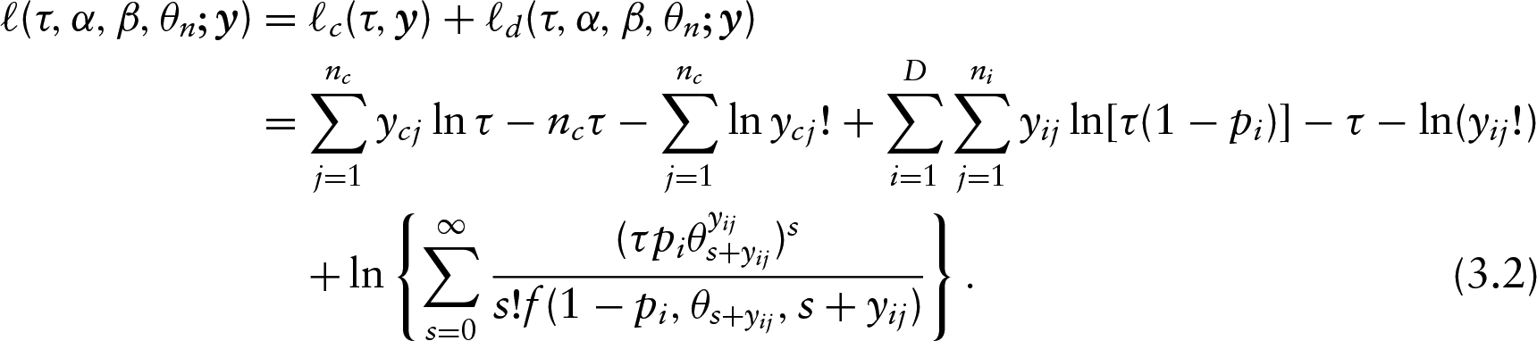
The counts from the zero-dose group will simply follow a Poisson distribution with parameter $τ$ . Thus the log-likelihood function for the counts from the zero-dose group is given by

ℓ_{c} = \sum_{j = 1}^{n_{c}} y_{cj} ln τ - n_{c} τ - \sum_{j = 1}^{n_{c}} ln y_{cj}!,

Consider now an observation corresponding to a non-zero dose of the drug which follows an Altham–Poisson distribution. Then the log-likelihood function can be written as

ℓ (τ, p_{i}, θ_{n}; y_{ij}) = y_{ij} 1n (τ (1 - p_{i})) - τ - ln (y_{ij}!) + ln \{\sum_{s = 0}^{\infty} \frac{{[τ p_{i} θ_{s + y_{ij}}^{y_{ij}}]}^{s}}{s! f (1 - p_{i}, θ_{s + y_{ij}}, s + y_{ij})}\} .

The log-likelihood for the data is found by summing the log-likelihood functions for each observation over all of the observed responses and is given by

\begin{matrix} ℓ (τ, α, β, θ_{n};) & = & ℓ_{c} (τ,) + ℓ_{d} (τ, α, β, θ_{n};) \\ = & \sum_{j = 1}^{n_{c}} y_{cj} ln τ - n_{c} τ - \sum_{j = 1}^{n_{c}} ln y_{cj}! + \sum_{i = 1}^{D} \sum_{j = 1}^{n_{i}} y_{ij} ln [τ (1 - p_{i})] - τ - ln (y_{ij}!) \\ + ln \{\sum_{s = 0}^{\infty} \frac{{(τ p_{i} θ_{s + y_{ij}}^{y_{ij}})}^{s}}{s! f (1 - p_{i}, θ_{s + y_{ij}}, s + y_{ij})}\} . \end{matrix}

(3.2)

The parameters of the Altham–Poisson distribution can be estimated by maximizing the log-likelihood function, where the infinite sum in expression (3.2) can be approximated by a finite sum and where a cutoff value for $s$ is selected so that a specified degree of accuracy is achieved. A numerical optimization routine can then be used to optimize the log-likelihood function in order to estimate the parameters of the model. Standard errors of these parameter estimates can be obtained from the Hessian matrix. The fit of the Altham–Poisson distribution can be compared with those of other models using AIC together with plots of Pearson residuals against fitted values.

An alternative method of estimating the parameters of the Altham–Poisson distribution is to use the EM algorithm but this algorithm was slow to converge (in accordance with Nelder (1977)) and hence the log-likelihood function was optimized directly in order to obtain parameter estimates. Indeed it is cogently argued that direct numerical maximization of a likelihood or log-likelihood is often to be preferred to the implementation of the the EM algorithm (MacDonald, 2014). The formulation of an EM algorithm for the Altham–Poisson distribution is subtle and somewhat complicated and full details are available in Leask (2009).

3.4 Example

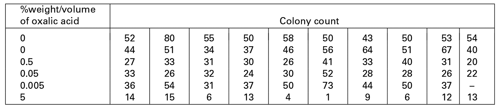
Trajstman (1989) presented data obtained from a study on bovine tuberculosis in Australia. Samples of bovine tissue were placed on culture plates and the growth of Mycobacterium bovis observed. Mycobacterium bovis grows slowly and is often overtaken by contaminants. As a result, culture plates need to be decontaminated prior to a study and a suitable dose of a decontaminant which kills as few Mycobacterium bovis organisms as possible is sought. The data includes colony counts of Mycobacterium bovis exposed to varying doses of the decontaminant oxalic acid for 12 weeks (Dataset 3, Appendix C).

Morgan (1992) considered these data and concluded that they are overdispersed. In order to accommodate the overdispersion present in the data, the Altham–Poisson distribution was used to model the data. A logit-link function was deemed most suitable and the probability of death $p_{i}$ at log-dose $x_{i} = 1, \dots, D$ , was modelled in terms of the log-dose administered as

p_{i} = \frac{e^{α + β x_{i}}}{1 + e^{α + β x_{i}}}, for i = 1, \dots, D .

In addition the parameter

θ_{n}

was modelled as a function of

n

using the log-link function

ln (θ_{n}) = γ_{0} + γ_{1} n

. The parameter

γ_{0}

was, however, found to be not significantly different from zero and was therefore dropped from the model for

θ_{n}

The standard errors of the parameter estimates were used to compute 95% Wald intervals for each of the parameters $τ, α, β$ and $γ_{1}$ . Profile likelihood plots were obtained for each of the parameters and these plots were used to obtain profile likelihood interval estimates for the parameters. The parameter estimates, together with their standard errors, 95% Wald confidence intervals and 95% profile likelihood intervals are recorded in Table 3. The estimate of $τ$ of $51.058$ is in accord with the nature of the data and indicates that the normal approximation to the Poisson distribution could well be invoked to some advantage in the analysis. However, since the emphasis here is on discrete distributions, this insight was not explored.

Table 3
Results from fitting the Altham–Poisson model to the bovine data.

Parameter Estimate Standard Error 95% Wald Interval 95% Profile Interval

$τ$ 51.058 1.493 $(48.132; 53.984)$ $(48.270; 54.210)$

$α$ 0.077 0.049 $(- 0.019; 0.173)$ $(- 0.023; 0.197)$

$β$ 0.138 0.043 $(0.054; 0.222)$ $(0.065; 0.240)$

$γ_{1}$ $- 0.0006$ $7.309 \times 10^{- 5}$ $(- 0.0007; - 0.0005)$ $(- 0.0008; - 0.0005)$

Parameter	Estimate	Standard Error	95% Wald Interval	95% Profile Interval
$τ$	51.058	1.493	$(48.132; 53.984)$	$(48.270; 54.210)$
$α$	0.077	0.049	$(- 0.019; 0.173)$	$(- 0.023; 0.197)$
$β$	0.138	0.043	$(0.054; 0.222)$	$(0.065; 0.240)$
$γ_{1}$	$- 0.0006$	$7.309 \times 10^{- 5}$	$(- 0.0007; - 0.0005)$	$(- 0.0008; - 0.0005)$

Source: Authors' computation.

Table 4

A comparison of the various models fitted to the bovine data.

Model	Maximum log-likelihood	Number of parameters	AIC
Poisson	$- 236.42$	3	478.8
Negative binomial	$- 217.28$	4	442.6
Altham–Poisson	$- 219.23$	4	446.5

Source: Authors' computation.

The Poisson and the negative binomial distributions derived to accommodate Wadley's problem (Anscombe 1949; Wadley 1949) were also fitted to the bovine data. Plots of Pearson residuals against fitted values for the these models, together with that for the Altham–Poisson distribution, are shown in Figure 3. The plots indicate that the adequacy of fit of the negative binomial and the Altham–Poisson models to the data are comparable and are substantially better than that of the Poisson-based model. AIC values for the three models are presented in Table 4 and indicate that the negative binomial is to be preferred over the Altham–Poisson model, albeit marginally. The latter result could be construed as disappointing. However, it may well be that the Altham–Poisson model is not entirely suitable for the particular dataset. (Lindsey and Altham (1998)) make a similar observation when comparing binomially-based models in a related context.

Figure 3

Source: Authors' computation.

4 Conclusions

The focus of this article is on the multiplicative binomial distribution introduced by Altham in 1978 and on its use in modelling over- and underdispersion in count data, dose–response data and data generated from a Wadley's problem setting. Some new results relating to the distribution are presented, thereby complementing the work of Altham (1978) and the findings reported in Feirer et al. (2013). The main results of the article, however, relate to the use of the multiplicative binomial distribution in modelling Wadley's problem, with the number of trials taken to be a Poisson variable. The distribution so obtained, termed the Altham–Poisson distribution, has not been derived or studied before and proved to be somewhat intractable algebraically. Properties of the model were, therefore, investigated numerically and its performance illustrated using a well-known benchmark dataset initially introduced by Trajstman (1989).

There is some scope for further research. Thus the quasi-likelihood approach of Wedderburn (1974), which is empirical in nature and which models the mean and variance of the underlying distribution separately, could be embedded in Wadley's problem in place of the multiplicative binomial distribution. In addition, distributions other than the Poisson, such as, the negative binomial distribution or the Conway-Maxwell-Poisson distribution (Shmueli et al., 2005), could be used to model the unobserved number of trials in a Wadley's problem setting, together with the multiplicative binomial distribution. In this way two potential sources of over- or under dispersion can be coupled and modelled. On a cautionary note however, the resultant distributions are expected to be somewhat complicated and may well be difficult to handle computationally.

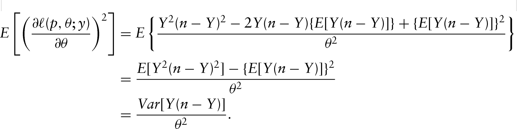
Appendix A: Information Matrix for the Multiplicative Binomial Distribution

Consider the individual entries of the information matrix for a single observation from the multiplicative binomial model.

\begin{matrix} E [{(\frac{\partial ℓ (p, θ; y)}{\partial p})}^{2}] & = & E [\frac{{[Y - E (Y)]}^{2}}{p^{2} {(1 - p)}^{2}}] \\ = & \frac{Var (Y)}{p^{2} {(1 - p)}^{2}} \\ E (\frac{\partial ℓ (p, θ; y)}{\partial p} \frac{\partial ℓ (p, θ; y)}{\partial θ}) & = & \frac{- n {[E (Y)]}^{2} + E (Y^{2}) E (Y) + nE (Y^{2}) - E (Y^{3})}{θ p (1 - p)} \\ = & \frac{E [Y^{2} (n - Y)] - E [Y (n - Y)] E (Y)}{θ p (1 - p)} \\ = & \frac{Cov [Y (n - Y), Y]}{θ p (1 - p)} \end{matrix}

and

\begin{matrix} E [{(\frac{\partial ℓ (p, θ; y)}{\partial θ})}^{2}] & = & E \{\frac{Y^{2} {(n - Y)}^{2} - 2 Y (n - Y) {E [Y (n - Y)]} + {E [Y (n - Y)]}^{2}}{θ^{2}}\} \\ = & \frac{E [Y^{2} {(n - Y)}^{2}] - {E [Y (n - Y)]}^{2}}{θ^{2}} \\ = & \frac{Var [Y (n - Y)]}{θ^{2}} . \end{matrix}

Appendix B: Approximating the Infinite Sum in the p.m.f. of the Altham–Poisson Distribution

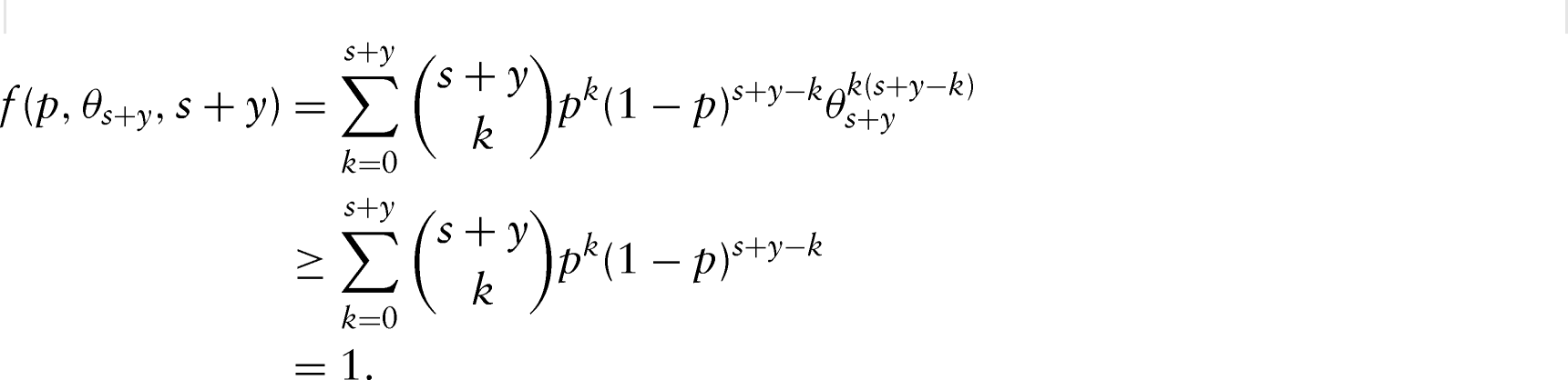
Shmueli et al. (2005) considered the Conway-Maxwell-Poisson distribution which is a weighted Poisson distribution and includes an infinite sum. In accordance with their work, an upper bound on the error that results from approximating the infinite sum with a finite sum in the p.m.f. of the Altham–Poisson distribution is sought. If an upper bound on the error term can be determined, the accuracy of the approximation can be controlled. Since the model reduces to a Poisson distribution when $θ_{n} = 1$ , consider the component $f (p, θ_{s + y}, s + y)$ in expression (3.1) for the two cases $θ_{s + y} > 1$ and $θ_{s + y} < 1$ .

When $θ_{s + y} > 1$ it follows that $θ_{s + y}^{k (s + y - k)} \geq 1$ , where $k$ is a positive integer and as a result

\begin{matrix} f (p, θ_{s + y}, s + y) & = & \sum_{k = 0}^{s + y} (\begin{matrix} s + y \\ k \end{matrix}) p^{k} {(1 - p)}^{s + y - k} θ_{s + y}^{k (s + y - k)} \\ \geq & \sum_{k = 0}^{s + y} (\begin{matrix} s + y \\ k \end{matrix}) p^{k} {(1 - p)}^{s + y - k} \\ = & 1 . \end{matrix}

Thus

\frac{{[τ θ_{s + y}^{y} (1 - p)]}^{s}}{s! f (p, θ_{s + y}, s + y)} \leq \frac{{[τ θ_{s + y}^{y} (1 - p)]}^{s}}{s!} .

(B.1)

Now consider again writing the infinite sum from expression (3.1) as

\sum_{s = 0}^{\infty} \frac{{[τ θ_{s + y}^{y} (1 - p)]}^{s}}{s! f (p, θ_{s + y}, s + y)} = \sum_{s = 0}^{k} \frac{{[τ θ_{s + y}^{y} (1 - p)]}^{s}}{s! f (p, θ_{s + y}, s + y)} + R_{k},

where

R_{k}

is the error or remainder term given by

R_{k} = \sum_{s = k + 1}^{\infty} \frac{{[τ θ_{s + y}^{y} (1 - p)]}^{s}}{s! f (p, θ_{s + y}, s + y)} .

From (B.1) it follows that

\begin{matrix} R_{k} & \leq & \sum_{s = k + 1}^{\infty} \frac{{[τ θ_{s + y}^{y} (1 - p)]}^{s}}{s!} \\ = & e^{[τ θ^{y} (1 - p)]} - \sum_{s = 0}^{k} \frac{{[τ θ_{s + y}^{y} (1 - p)]}^{s}}{s!} . \end{matrix}

The remainder term

R_{k}

therefore has an upper bound that is computable when

θ_{s + y} > 1

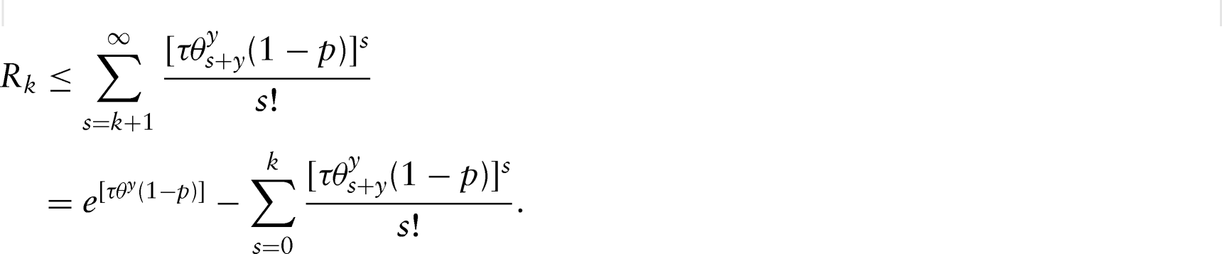
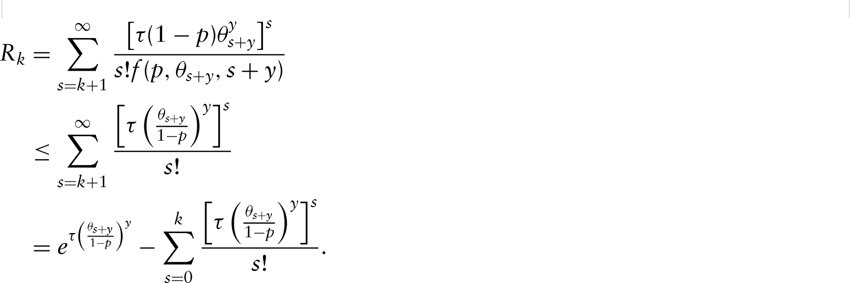
The inequality $θ_{s + y}^{k (s + y - k)} \geq θ_{s + y}^{k (s + y)}$ holds for values of $θ_{s + y}$ that are less than one. Therefore

\begin{matrix} f (p, θ_{s + y}, s + y) & \geq & \sum_{k = 0}^{s + y} (\begin{matrix} s + y \\ k \end{matrix}) p^{k} {(1 - p)}^{s + y - k} θ_{s + y}^{k (s + y)} \\ = & {(1 - p + p θ_{s + y}^{s + y})}^{s + y}, \end{matrix}

and hence

\begin{matrix} \frac{{[τ (1 - p) θ_{s + y}^{y}]}^{s}}{s! f (p, θ_{s + y}, s + y)} & \leq & \frac{{[τ (1 - p) θ_{s + y}^{y}]}^{s}}{s! {(1 - p + p θ_{s + y}^{s + y})}^{s + y}} \\ = & \frac{{[τ θ_{s + y}^{y}]}^{s}}{s! {(1 + \frac{p}{1 - p} θ_{s + y}^{s + y})}^{s + y} {(1 - p)}^{y}} \\ \leq & \frac{{[τ θ_{s + y}^{y}]}^{s}}{s! {(1 - p)}^{y}} since \frac{p}{1 - p} θ_{s + y}^{s + y} > 0 \\ \leq & \frac{{[τ {(\frac{θ_{s + y}}{1 - p})}^{y}]}^{s}}{s!} . \end{matrix}

Consider partitioning the infinite sum in the following way

\sum_{s = 0}^{\infty} \frac{{[τ (1 - p) θ_{s + y}^{y}]}^{s}}{s! f (p, θ_{s + y}, s + y)} = \sum_{s = 0}^{k} \frac{{[τ (1 - p) θ_{s + y}^{y}]}^{s}}{s! f (p, θ_{s + y}, s + y)} + R_{k},

where the remainder,

R_{k}

, is written as

\begin{matrix} R_{k} & = & \sum_{s = k + 1}^{\infty} \frac{{[τ (1 - p) θ_{s + y}^{y}]}^{s}}{s! f (p, θ_{s + y}, s + y)} \\ \leq & \sum_{s = k + 1}^{\infty} \frac{{[τ {(\frac{θ_{s + y}}{1 - p})}^{y}]}^{s}}{s!} \\ = & e^{τ {(\frac{θ_{s + y}}{1 - p})}^{y}} - \sum_{s = 0}^{k} \frac{{[τ {(\frac{θ_{s + y}}{1 - p})}^{y}]}^{s}}{s!} . \end{matrix}

Thus when

θ < 1

R_{k}

is bounded above and the bound is computable.

Therefore, the remainder term $R_{k}$ has an upper bound for all values of $θ_{s + y}$ and as a result the infinite sum in (3.1) can be approximated by a finite sum with cutoff $s_{cut}$ . For a predetermined upper bound on the remainder term an associated value for $s_{cut}$ can be obtained, thereby ensuring that the finite sum approximates the infinite sum with a desired degree of accuracy.

Appendix C: Datasets

Dataset 1: Geissler's data: the number of boys born to 6115 families of 13 children with the last birth not included (Edwards, 1958).

Number of boys	0	1	2	3	4	5	6	7	8	9	10	11	12
Number of families	3	24	104	286	670	1033	1343	1112	829	478	181	45	7

Dataset 2: Data for mice exposed to doses of trichloromethane (Morgan, 1992, p. 252 ).

Dosage (mg/kg)	Number dead per litter of 8
Control	0	0	0	2	2
250	0	0	1	3	6
300	0	0	0	1	8
350	0	2	2	5	8
400	1	2	4	6	7
450	1	4	5	6	8
500	1	7	8	8	8

Dataset 3: Colony counts of Mycobacterium bovis exposed to varying doses of the decontaminant oxalic acid for 12 weeks (Trajstman, 1989; Morgan, 1992).

%weight/volume of oxalic acid	Colony count
0	44	51	34	37	46	56	64	51	67	40
0.5	27	33	31	30	26	41	33	40	31	20
0.05	33	26	32	24	30	52	28	28	26	22
0.005	36	54	31	37	50	73	44	50	37	–
5	14	15	6	13	4	1	9	6	12	13

Footnotes

Acknowledgments

The authors would like to thank the Editor, the Associate Editor and two reviewers for their insightful comments which did much to enhance the content and readability of the paper. The authors would also like to thank the University of KwaZulu-Natal, the University of Cape Town, the Centre for the AIDS Programme of Research in South Africa (CAPRISA) and the National Research Foundation (NRF) of South Africa, grant (UID) 85456, for financial support. Any opinion, finding and conclusion or recommendation expressed in this material is that of the authors and the NRF does not accept liability in this regard.

References

Altham

PME

(1978) Two generalizations of the binomial distribution. Journal of the Royal Statistical Society, Series C (Applied Statistics) , 27, 162–67.

Anscombe

(1949) The statistical analysis of insect counts based on the negative binomial distribution. Biometrics , 5, 165–73.

Azzalini

(1996) Statistical inference based on the likelihood . London: Chapman and Hall.

Böhning

Baksh

Lerdsuwansri

Gallagher

(2013) Use of the ratio plot in capture-recapture estimation. Journal of Computational and Graphical Statistics , 22, 135–55.

Collett

(2003) Modelling binary data .London: Chapman and Hall/CRC.

Cox

(1972) The analysis of multivariate binary data. Journal of the Royal Statistical Society, Series C (Applied Statistics) , 21, 113–20.

Edwards

AWF

(1958) An analysis of Geissler's data on the human sex ratio. Annals of Human Genetics , 23, 6–15.

Feirer

Friedl

Hirn

(2013) Modelling over- and underdispersed frequencies of successful ink transmissions onto paper. Journal of Applied Statistics , 40, 626–43.

Leask

(2009) Wadley's problem with overdispersion. Unpublished Ph.D. thesis: University of KwaZulu-Natal. Available from the author on request.

10.

Leask

Haines

(2014) The beta-Poisson distribution in Wadley's problem. Communications in Statistics: Theory and Methods , 43, 4962–71.

11.

Lindsey

(1995) Modelling frequency and count data . Oxford: Oxford University Press.

12.

Lindsey

Altham

PME

(1998) Analysis of the human sex ratio by using overdispersion models. Journal of the Royal Statistical Society, Series C (Applied Statistics) , 47, 149–57.

13.

Lovison

(1997) Some notes on binary data with overdispersion. Statistica Applicata , 9, 403–18.

14.

Lovison

(1998) An alternative representation of Altham's multiplicative-binomial distribution. Statistics & Probability Letters , 36, 415–20.

15.

MacDonald

(2014) Numerical maximisation of likelihood: A neglected alternative to EM? International Statistical Review , 82, 296–308.

16.

Molenberghs

Ryan

(1999) An exponential family model for clustered multivariate binary data. Environmetrics , 10, 279–300.

17.

Morgan

BJT

(1992) Analysis of quantal response data . London: Chapman and Hall.

18.

Nelder

(Discussant) (1977) Maximum likelihood from incomplete data via the EM algorithm. Journal of the Royal Statistical Society, Series B (Methodological) , 39, 23–24.

19.

Ord

(1967) Graphical methods for a class of discrete distributions. Journal of the Royal Statistical Society, Series A (General) , 130, 232–38.

20.

Shmueli

Minka

Kadane

Borle

Boatwright

(2005) A useful distribution for fitting discrete data: Revival of the Conway-Maxwell-Poisson distribution. Applied Statistics , 54, 127–42.

21.

Skellam

(1948) A probability distribution derived from the binomial distribution by regarding the probability of success as variable between the sets of trials. Journal of the Royal Statistical Society, Series B (Methodological) , 10, 257–61.

22.

Trajstman

(1989) Indices for comparing decontaminants when data come from dose–response survival and contamination experiments. Applied Statistics , 38, 481–94.

23.

Wadley

(1949) Dosage-mortality correlation with number treated estimated from a parallel sample. Annals of Applied Biology , 36, 196–202.

24.

Wedderburn

RWM

(1974) Quasi-likelihood functions, generalized linear models, and the Gauss-Newton method. Biometrika , 61, 439–47.

25.

Williams

(1975) The analysis of binary responses from toxicological experiments involving reproduction and teratogenicity. Biometrics , 31, 949–52.

26.

Zelterman

(2004) Discrete distributions: Applications in the health sciences . Chichester: Wiley.