This article addresses estimation in regression models for longitudinally collected functional covariates (time-varying predictor curves) with a longitudinal scalar outcome. The framework consists of estimating a time-varying coefficient function that is modelled as a linear combination of time-invariant functions with time-varying coefficients. The model uses extrinsic information to inform the structure of the penalty, while the estimation procedure exploits the equivalence between penalized least squares estimation and a linear mixed model representation. The process is empirically evaluated with several simulations and it is applied to analyze the neurocognitive impairment of human immunodeficiency virus (HIV) patients and its association with longitudinally-collected magnetic resonance spectroscopy (MRS) curves.
Technological advancements and increased availability of storage of large datasets have allowed for the collection of functional data as part of time course or longitudinal studies. In the cross-sectional setting, there have been many proposed methods for estimating a regression function in a so-called functional linear model (fLM). This function is a continuous analogue of a vector of (discrete) regression coefficients; it connects the scalar response, to a functional covariate, . Although estimation for fLMs has been well studied, the extension to longitudinally collected functions has not received much attention. Only recently have longitudinal penalized functional regression (LPFR) and longitudinal functional principal component regression (LFPCR) approaches have been proposed to extend the cross-sectional fLM to a longitudinal setting by incorporating subject-specific random intercepts (Goldsmith et al., 2012; Gertheiss et al., 2013). However, a basic assumption of LPFR and LFPCR is that the regression function remains constant over time. Consequently, these methods are not suited for situations in which the association between a functional predictor and scalar response may evolve over time. We propose a technique that extends the analysis of fLMs by relating a scalar outcome to a functional predictor—both observed longitudinally—and estimates a time-dependent regression function.
The method fits into a generalized ridge regression framework by incorporating an scientifically informed context-dependent quadratic penalty term into the estimation process. Our extension of the fLM framework to the longitudinal setting has two major advantages: (a) the regression function is allowed to vary over time and (b) extrinsic, scientifically relevant information about the structure of the regression function can be incorporated directly into the estimation process. We formulate the estimation procedure within a mixed-model framework, making the method computationally efficient and easy to implement.
Ramsay and Dalzell (1991) introduced the term functional data analysis (FDA) in the statistical literature. The cross-sectional fLM with scalar response can be stated as follows (see, e.g., Yao and Müller, 2010):
where is the mean of , denotes the domain of the predictor functions , and is a square integrable function that models the linear relationship between the functional predictor and scalar response. We will assume that denotes a mean-centred function ( for almost all ).
As there is no unique that solves this equation, some form of regularization or constraint is required. A common constraint is to impose smoothness on . One approach to this is to expand both the regression function and predictor functions in terms of B-splines and then obtain the regularized estimate of (Ramsay and Silverman, 1997). Another approach is to express the regression function in terms of the empirical orthonormal basis obtained by the eigenfunctions of the covariance of (i.e., a Karhunen—Loève (K—L) expansion (e.g., Müller, 2005). A third approach, known as penalized functional regression (PFR) (Goldsmith et al., 2011), combines the above two methods. In PFR, a spline basis is used to represent and a subset of empirical eigenfunctions is used to represent each . Another approach is to use a wavelet basis, instead of splines or eigenfunctions, to represent the predictor functions (Morris and Carroll, 2006).
Here we adopt an approach by Randolph et al. (2012) that does not begin by explicitly projecting onto a pre-specified subspace of functions. Instead, prior information about this subspace and its inherent functional structure is incorporated into the estimation process by way of a penalty operator, . This approach of partially empirical eigenvectors for regression (PEER) exploits the fact that a penalized least squares regression estimate mathematically arises as a series expansion in terms of a set of basis functions determined jointly by the covariance (empirical functional structure) and the penalty (imposed structure). This naturally extends ridge regression (non-structured penalty) and smoothing penalties such as a second-derivative penalty (presuming a smooth regression function). Here we extend the scope of the PEER approach to the longitudinal setting in a manner that allows the estimated regression function to vary with time. Our interest lies primarily in the estimation of a regression function rather than the prediction of an outcome ; see, for example, Cai and Hall, (2006) for a discussion regarding the substantially different characteristics of these two goals.
The problem we address involves repeated observations from each of subjects. For each subject, , at each observation time, , we collect data on a scalar response variable, , and a (idealized) predictor function, . We are interested in longitudinal regression models of the form:
denotes the regression function at time and is a vector of scalar-valued (non-functional) predictors. and denote the subject-specific random effect and random error term, respectively. In a spirit similar to that of a linear mixed model with time-related slope for longitudinal data, we assume that can be decomposed into several time-invariant component functions, for example, .
Our work is motivated by a study in which magnetic resonance (MR) spectra have been collected longitudinally from late-stage human immunodeficiency virus (HIV) patients (Harezlak et al., 2011). We consider global deficit score (GDS) as a scalar response variable, , and MR spectra as predictor functions, . The association of GDS with MR spectra and how this association evolves with time are of interest. One MR spectrum is shown in the left panel of Figure 1: The amplitude, , is plotted against the frequency , normalized to the interval (-axis). The pattern and amplitudes of the peaks contain information about the concentration of metabolites present in tissue. Each metabolite has a unique spectrum and so one MR spectrum is a mixture of spectra from each individual metabolite (plus background and random noise); see the right panel in Figure 1 that displays spectra from nine metabolites. Consequently, one expects an observed spectrum from tissue to lie near a functional subspace, , spanned by the spectra of pure metabolites. The regression function, , models the association between and and hence, in principle, should also lie near . Hence, the subspace should be more informative than B-splines or cosine functions that are in some sense ‘external’ to the problem. For this reason, we adopt a methodology that encourages the estimate of to be in or near the preferred subspace, . The approach is implemented using a decomposition-based penalty, , which penalizes the estimate of lightly if it belongs to and strongly if it does not (Randolph et al., 2012).
Left panel: An observed MR spectrum from tissue. Right panel: The nine pure metabolite spectra. In each plot, the -axis represents amplitude and -axis the frequency of nucleus, , normalized to interval.
The cross-sectional fLM with scalar response has been a focus of various investigations (Faraway, 1997; Ramsay and Silverman, 1997; Fan and Zhang, 2000; Cardot et al., 1999, 2003; Cai and Hall, 2006; Cardot et al., 2007; Reiss and Ogden, 2009), many of which estimate a regression function in two steps. For example, Cardot et al. (2003) first perform principal component regression (PCR), which projects the observed predictor curves onto an empirical basis to obtain an estimate and then use B-splines to smooth the result. Reiss and Ogden, (2009) study several of these methods along with modifications that include versions of PCR using B-splines and second-derivative penalties (cf. Ramsay and Silverman, 1997; Silverman 1996). Extensions of fLM have been made towards generalized linear model with functional predictors (James, 2002; Müller and Stadtmüller, 2005) and quadratic functional regression (Yao and Müller, 2010). We are interested in extending the fLM to a longitudinal setting. To our knowledge, the only published methods addressing the longitudinal functional predictor framework are LPFR (Goldsmith et al., 2012) and LFPCR (Gertheiss et al., 2013). However, both LPFR and LFPCR assume that the regression function in equation (1.1), , remains constant over time. In contrast, proposed estimate is based on modelling the regression function as a time-dependent linear combination of several time-invariant component functions, , each of which is estimated via a penalty operator, , that is informed by the context of the scientific question.
An important concern for any regularized estimation method, either cross-sectional or longitudinal, is identifiability of the estimate, that is, the lack of uniqueness or, possibly, its instability. In the fLM, this arises from the lack of invertibility of the empirical covariance operator. A finite number of predictor curves means the dimension of the range of this operator is finite and so, as an operator on a infinite-dimensional domain, it has a non-trivial null space. The philosophy behind a penalty-operator approach is that estimation is constrained to the subspace spanned by functions that are jointly determined by and . A sufficient condition for uniqueness of this estimate is to assume (Bjorck, 1996; Engl et. al., 2000). We assume this throughout.
Longitudinal functional regression model with time-varying regression function is described in Section 2. In Section 3.1, estimate of regression function is obtained as a generalized ridge estimate (Tikhonov, 1963; Hoerl and Kennard, 1970). Concept of decomposition-based penalty is reviewed in Section 3.2. We have described mixed model approach of estimation as best linear unbiased predictors (BLUP) in Section 4.1 and expressions for the precision of the estimates are derived in Section 4.2. In the supplemental material (available online in journal's website), we present how our longitudinal penalized estimate, along with its bias and precision, can be obtained, under some weak assumptions, in terms of generalized singular vectors.
Simulation results are presented in Section 5. An application to real magnetic resonance spectroscopy (MRS) data using, and a summary of our findings, is presented in Section 6. The methods discussed in this paper have been implemented in the R package refund (Crainiceanu et al., 2012) via the peer() and lpeer() functions.
Statistical model
Let denote a continuous predictor function defined on the closed interval , without loss of generality . Let denote a predictor function from the ith subject () at the ith timepoint (). Technically, an observed predictor arises as a discretized sampling from an idealized function and we will assume that each observed predictor is sampled at the same locations, , with sampling that is appropriately regular and dense enough to capture informative functional structure, as seen, for instance, in the MRS data in Section 6. Let be the vector of values sampled from the realized function . Then, the observed data are of the form , where is a scalar outcome, is a column vector of measurements on scalar predictors and is the sampled predictor from the ith subject at time . Denoting the true regression function at time by , the longitudinal functional outcome model of interest is
where and is the vector of random effects pertaining to subject and distributed as . As usual, we assume that is a subset of , and are independent, and are independent whenever or or both and and are independent if . Here, is the standard fixed effect from univariate predictors, is the standard random effect and is the subject/time-specific functional effect. We assume that for all , is a twice-continuously differentiable function of .
The functional structure, indexed by , and time structure, indexed by , have somewhat unequal roles in our model, as we assume that the longitudinal observations are more limited in the amount of information relative to the densely sampled index. For example, may vary linearly with time, , or quadratically, . This is similar in spirit to a linear mixed effects model with linear or quadratic time slope (see, e.g., Fitzmaurice et al., 2004). In general, we assume that can be decomposed into several time-invariant component functions as
where, are prescribed linearly independent functions of and for all ; the time component enters into through these terms. At , reduces to and has the obvious interpretation of a baseline regression function. When , is independent of , a situation considered by Goldsmith et al. (2012). In general, each may be any function of with , for example, or . We rewrite equation (2.1) as
The association of with is modelled as a linear dependence on observations at sampling points, . In our approach, the (functional) structure is imposed directly into the estimation of each , for (as described in Section 3). Combining all observations from the subjects obtained across all timepoints, we express this model in discretized matrix form as
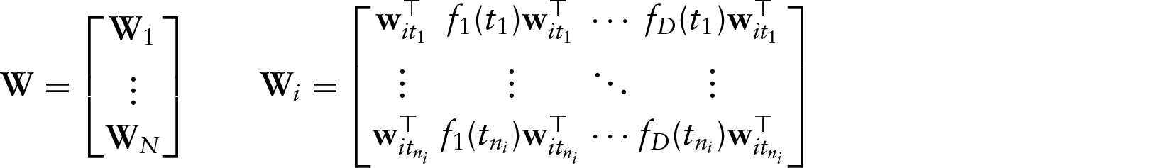
Here, is a vector of all responses, is an design matrix pertaining to univariate predictors, is the associated coefficient vector, is a coefficient vector representing a discretized, structured association between the sampled curves and . Further, is vector of random effects and is corresponding design matrix. The matrix has the form
The first set of columns of is obtained as follows: (a) first, place all the observed values of from first subject collected at first timepoint in the first row; (b) then, place the observed values of from all the timepoints and all the subjects in the successive rows in such a way that each row represents observed value of from a specific timepoint and subject, and the rows are ordered by time and subjects according to . Once the first set of columns is constructed, the second set of columns is constructed by multiplying first columns by . Similarly, the third set of columns is constructed by multiplying first columns by and so on.
Estimation of parameters with a penalty
The proposed estimation approach builds on intuition from single-level functional regression that encourages an estimate of to be in or near a ‘preferred’ space via choice of penalty operator (Randolph et al., 2012). To describe the effect of a general penalty operator, , it is useful to consider the familiar example of a Laplacian penalty, . The typical heuristic for this arises by viewing as a function whose local ‘smoothness’ is informative. In this case, the term penalizes sharp changes in . For our perspective, it is helpful to recall that the dominant eigenvectors of (those corresponding to the largest eigenvalues) are sharply oscillatory while the least dominant eigenvectors are very smooth. Hence a linear-algebraic view of this is that rather than penalizing sharp changes, smoothness in the estimate is inherited from the eigenproperties of . More specifically, structure in the estimate arises from the joint eigenproperties of and ; this is given by the generalized singular value decomposition (GSVD), as described in the Supplemental section. In general, the least-dominant eigenfunctions of a penalty will have the largest effect on the estimate. This property can be used to construct a ‘preferred subspace’ by defining a penalty whose least dominant (or perhaps zero-associated) eigenfunctions are preferred. The estimates of are obtained as follows: (a) identify the ‘preferred’ functional subspace where is expected to belong; (b) define a decomposition-based penalty (see Section 3.2) to encourage the estimate to be close to and (c) obtain a penalized estimate of . We say ‘encourage’ rather than ‘constrain’ because the estimate is not forced to be in a subspace , but rather it is jointly determined by and (as illustrated in Section 5.4). Proposed approach allows different preferred subspace for each of s. In the longitudinal (or ) dimension, is more explicitly and severely constrained by the choice of .
Generalized ridge estimate
The model described in Section 2 can be written as
where and . For each , let be the penalty operator for and let be the associated tuning parameter. The corresponding penalized estimates of and are minimizers of:
where for some symmetric, positive definite matrix . A generalized ridge estimate of and minimizing equation (3.2) is obtained as (see Ruppert et al., 2003)
where, , and . In the supplemental material, we have derived an expression for the generalized ridge estimate , explicitly in terms of the GSVD.
Decomposition-based penalty
Let be the estimate obtained from the penalty operator and tuning parameter , for each . For example, may denote (a ridge penalty) or a second-order derivative penalty (giving an estimate having continuous second derivative). Alternatively, with prior knowledge about potentially relevant structure in a regression function, a targeted decomposition-based penalty can be defined in terms of a subspace defined by such structure (Randolph et al., 2012). To be precise, if it is appropriate to impose scientifically informed constraints on the ‘signal’ being estimated by , this prior may be implemented by encouraging the estimate to be in or near a subspace, . We further assume that the subspace is spanned by the functions .
Returning to our notation that reflects functional predictors observed at sampling points, we represent by the range of a matrix whose columns are , where each represents the discretized . Consider the orthogonal projection onto the , where is Moore—Penrose inverse of . Then a decomposition penalty is defined as
for scalars and . To see how works, let be any estimate of . When , we have , but when , we have . The condition imposes more penalty for , compared to when . The weights and determine the relative strength of emphasizing in the estimation process. Note that is invertible, provided and are nonzero, and that results in ordinary ridge estimate.
Mixed model representation
We aim to construct an appropriate mixed model that minimizes the expression in equation (3.2). In general, the penalty, , is not required to be invertible but for simplicity, this will be assumed here. The mixed model approach provides an automatic selection of tuning parameters restricted maximum likelihood (REML)’based estimation of the tuning parameters has been shown to perform as well as other criteria and under certain conditions, it is less variable than generalized cross validation (GCV)’based estimation (Reiss and Ogden, 2009).
Estimation of parameters
Using Henderson's justification (Henderson, 1950), one can show that, for each , model , where and minimizes the expression (3.2) to obtain the BLUP. Thus, the generalized ridge estimate of and corresponds to the BLUP from the following model:
where, , and with and . This representation allows us to estimate fixed and functional predictors, simply by fitting a linear mixed model (e.g., using nlme package in R or PROC MIXED in SAS).
Precision of estimates
Our ridge estimate is the BLUP from an equivalent mixed model, hence the variance of the estimate depends on whether the parameters are random or fixed. Randomness of is a device used to obtain the ridge estimate while and in our case are truly random. With this in mind, we assume that the variance of the estimates is conditional on , but not on . The BLUP of , and can be expressed as (see, e.g., Robinson, 1991; Ruppert et al., 2003):
where . is an unbiased estimator of , but is not unbiased. It is trivial to see that . Thus, the conditional variances of and are:
To obtain the unconditional variance, one must replace by in the above expressions, but this will overestimate the variance of the estimates. The 95% confidence bands can be constructed as , using the expression for the standard error derived here. The constant was obtained by Salganik et al. (2004) through a large simulation study to ensure 95% simultaneous coverage.
Expressions for the predicted value of y and its variance are:
where Let, . Then the discretized version of regression function at time is . Therefore, the estimate of is and the estimate of its variance is .
Selection of time structure in
The proposed approach allows a flexible choice of the time structure to be included in the regression function . In practice, data and information to estimate structure of the longitudinal observations (along the index) are more limited than the functional relationship along the index. For example, whether is sufficient or the more flexible is required is not known. The problem of choosing appropriate time structure in is similar, in principle, to that of choosing time structure in a linear mixed-effects model (e.g., or ). We propose two approaches to determine the form of the unknown regression function: (a) use Akaike information criterion (AIC) to compare different structures and (b) use a point-wise confidence band for the component functions: . If the confidence band for any contains zero in its entire domain, then such term is dropped from the .
Selection of ϕa and ϕb for a decomposition penalty
We view and as weights of a trade-off between preferred and non-preferred subspaces and assume . In the current implementation, we use REML to estimate ’s for a fixed value of and perform a grid search over the values to jointly select the tuning parameters that maximize the information criterion, such as AIC, based on the restricted maximum likelihood.
Simulation
The proposed method of estimating regression function using decomposition-based penalty will be referred to as longitudinal partially empirical eigenvectors for regression (LongPEER). We pursue several simulations to evaluate its properties. The first simulation study (Section 5.1) compares the performance of LongPEER with the LPFR approach. In the remaining simulation studies, only LongPEER is considered due to a lack of comparable alternatives. The purpose of the second simulation study is to evaluate the influence of sample size and the contribution of prior information about the functional structure (as determined by the tuning parameters and in equation (3.4)) on the LongPEER estimate. In the third simulation study, we evaluate the coverage probabilities of the confidence bands constructed using the formula presented in Section 4.2. Finally, in Section 5.4, we evaluate the performance of a LongPEER estimate when information on some features is missing. These studies are performed in the context of MRS data and hence the simulated predictor functions are constructed based on the structure of MRS data. All results summarized in this section are based on 100 simulated datasets.
For each subject and visit, predictor functions were simulated using equation (5.3). Predictor functions were flat with bumps of varied widths at a number of pre-specified locations. White noise was added to the predictor functions to account for the instrumental measurement noise. These ‘bumpy’ regression functions were generated with bumps at some (but, not all) of the bump locations of the predictor function. For the simulation in Section 5.1, the regression function is assumed to be independent of time, whereas it varies with time in the simulation of Section 5.2. For both predictor and regression functions, 100 equispaced sampling points in [0,1] are used.
For the decomposition-based penalty (3.4), the matrix is defined as follows: (a) select the discretized functions spanning the ‘preferred’ subspace, where each is defined to have a single bump corresponding to a region in the simulated predictor functions (see Figure 2) and (b) compute , where . The columns of need not be orthogonal (cf. Figure 9). For ridge and second-order penalties, the matrices are defined as and , respectively, where is a square matrix with entries , and otherwise.
Our primary interest lies in estimation of regression function; therefore, estimation error is summarized in terms of the mean squared error (MSE) defined as , where denotes the estimate of . We also calculated the sum of squared prediction errors (SSPE) as , where denotes the estimate of the true (noiseless) to evaluate the prediction performance. The estimates based on the proposed methods, including the LongPEER estimate, were obtained as BLUPs from the mixed model formulation described in Section 4.1.
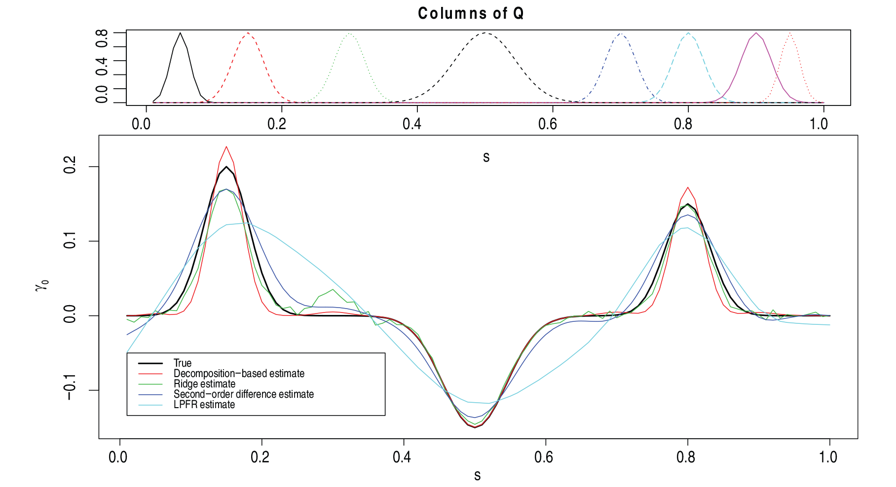
Average estimates of for the simulation as described in Section 5.1 with and . Top panel: Prior information used in LongPEER estimation. Bottom panel: True and the average estimates from 100 simulations. LongPEER, ridge and second-order difference estimates have been obtained using decomposition-based penalty, ridge penalty and second-order difference penalties, respectively, as described in third paragraph of Section 5. LPFR estimates were obtained using lpfr() with default options in refund package.
Comparison with LPFR
As mentioned, LPFR estimates a regression function that does not vary with time. Therefore, in order to compare LongPEER with LPFR, in the first set of simulations, we generated outcomes using a time-invariant regression function (i.e., , for all ). The following model was used to generate the outcome data for 100 individuals, each at 4 timepoints ():
We uniformly sampled ”” at . was defined with bumps centred at :
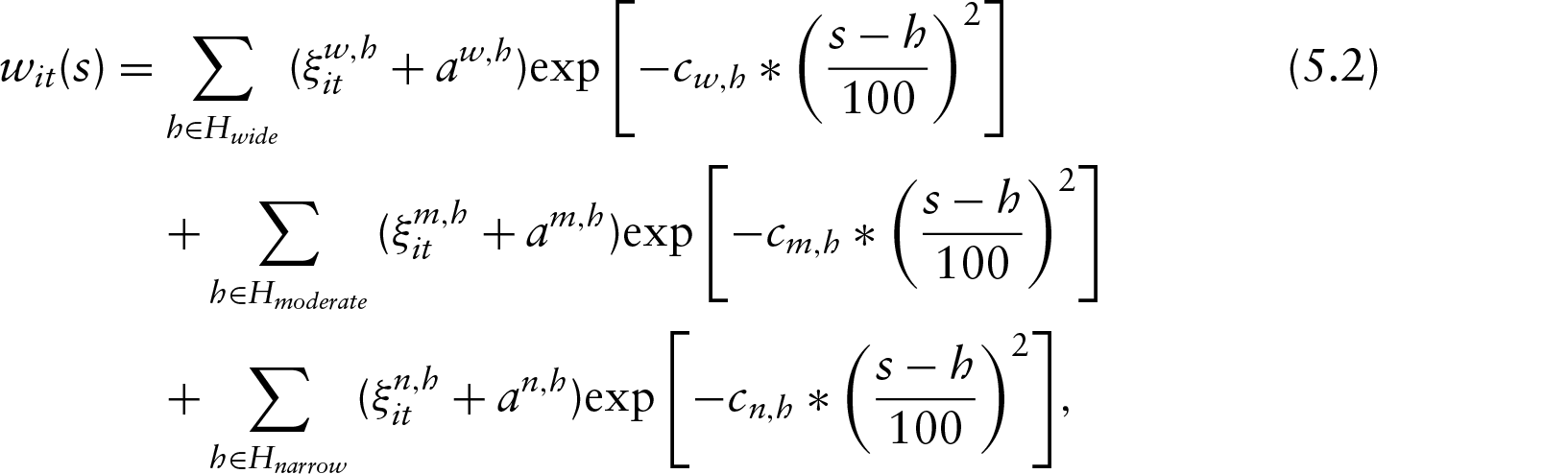
where and correspond to amplitude and degree of curvature, respectively, at the bumps, as specified in Table 1. We constructed to consist of wide, moderate and narrow bumps centred at: , and . Specifically, we generated the subject-specific functional predictors (i.e., the observed values of W) of the form
where , and correspond to the amplitude and degree of curvature at the wide, moderate and narrow bumps, respectively. These are defined in Table 1. Note that the amount of curvature in differs considerably from the amount imposed in and . , and were drawn independently from uniform(0, 0.1). Also, , and .
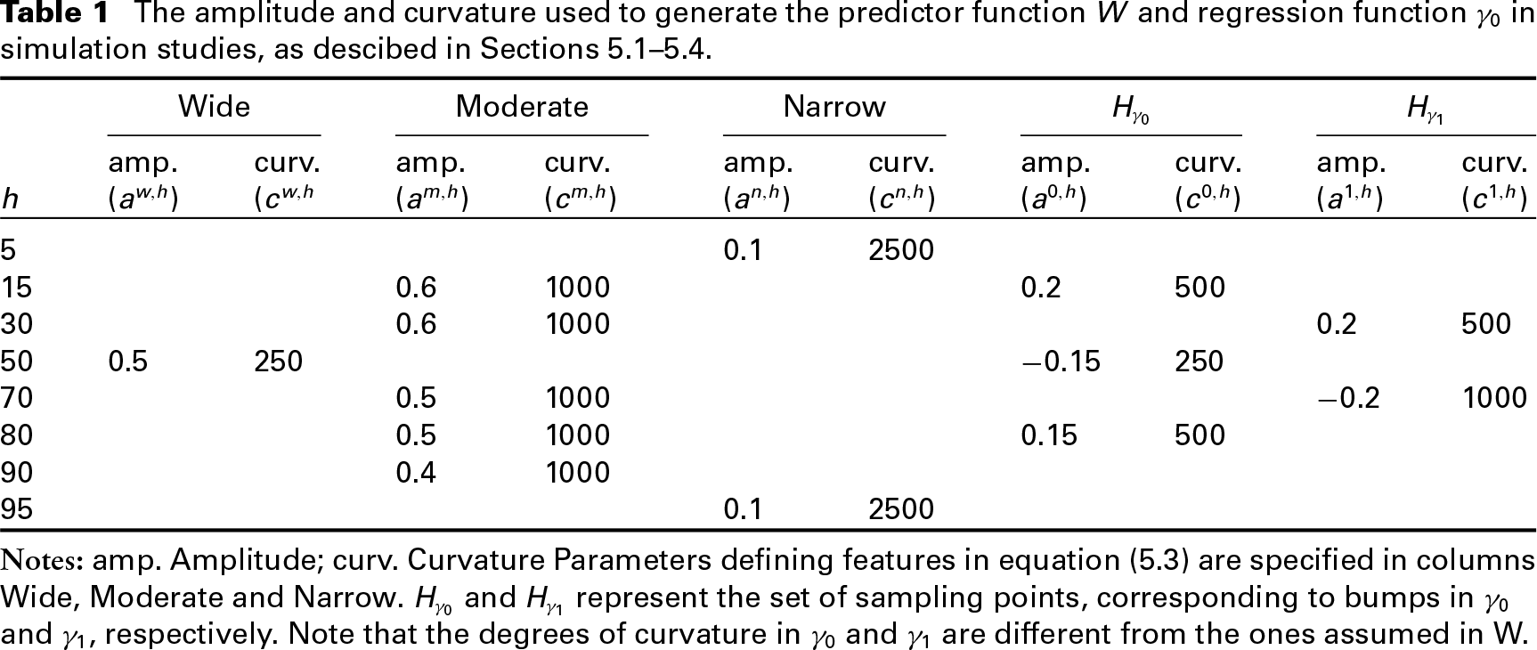
The amplitude and curvature used to generate the predictor function and regression function in simulation studies, as descibed in Sections 5.1–5.4.
Wide
Moderate
Narrow
amp.
curv.
amp.
curv.
amp.
curv.
amp.
curv.
amp.
curv.
h
5
0.1
2500
15
0.6
1000
0.2
500
30
0.6
1000
0.2
500
50
0.5
250
0.15
250
70
0.5
1000
0.2
1000
80
0.5
1000
0.15
500
90
0.4
1000
95
0.1
2500
Notes: amp. Amplitude; curv. Curvature Parameters defining features in equation (5.3) are specified in columns Wide, Moderate and Narrow. Hγ0 and Hγ1 represent the set of sampling points, corresponding to bumps in γ0 and γ1, respectively. Note that the degrees of curvature in γ0 and γ1 are different from the ones assumed in W.
Both LPFR (using lpfr() available in the refund package in R (Crainiceanu et al., 2012)) and the LongPEER estimates were obtained. For LPFR estimate, the dimension of both principal components and truncated power series spline basis were set to 30. The prior information used here is represented by bumps of various scalings and locations, as shown in the top panel of Figure 2. This structure is loosely consistent with that present in the predictors. We used , a choice motivated by our findings in Sections 5.2 and 5.4.
Table 2 displays the MSE and prediction error obtained for LongPEER and LPFR estimates. The SSPE was similar for both methods (1.1572 and 1.1527); however, the LongPEER estimate has smaller MSE. Both bias and variance are higher for the LPFR estimate and consequently it has the greater MSE. Figure 2 displays the estimates of the regression function. It should be emphasized that any comparison of these methods is not entirely fair since LongPEER is designed to exploit presumed structural information while LPFR is not. We, note that the ability to exploit such information may be limited and so in this simulation we used imprecise information about the shapes of features; see top panel in Figure 2.
Estimation and prediction errors for LPFR and LongPEER estimates based on 100 simulated datasets. The sample size is and the number of longitudinal observations is .
LongPEER
LPFR
0.0257
0.2229
0.0057
0.0653
0.0200
0.1576
1.1572
1.1527
Simulation with a time-varying regression function
Here and in subsections 5.3 and 5.4, the regression function varies parametrically with time. Due to the lack of existing alternatives for time-varying functional regression for comparison, we instead evaluate the performance of our approach in several ways. First, our primary goal was to assess the effects of sample size, fraction of variance explained by the model and the relative contribution of extrinsic information (as determined by and in equation (3.4)) on estimate. Without loss of generality, we set and vary on an exponential scale. Larger values of indicate greater emphasis of prior information on the estimation process. The model considered here was similar to that described in Section 5.1, with the exception that . The function is defined in equation (5.1) and was defined with bumps centred at
where and correspond to amplitude and degree of curvature, respectively, at the bumps as specified in Table 1. As before, it was assumed that . Realizations of functional predictors were generated, as described in Section 5.1. For each simulation, an appropriate was chosen to ensure that the squared multiple correlation coefficient is and . Here, denotes the average sample variance in the set with .
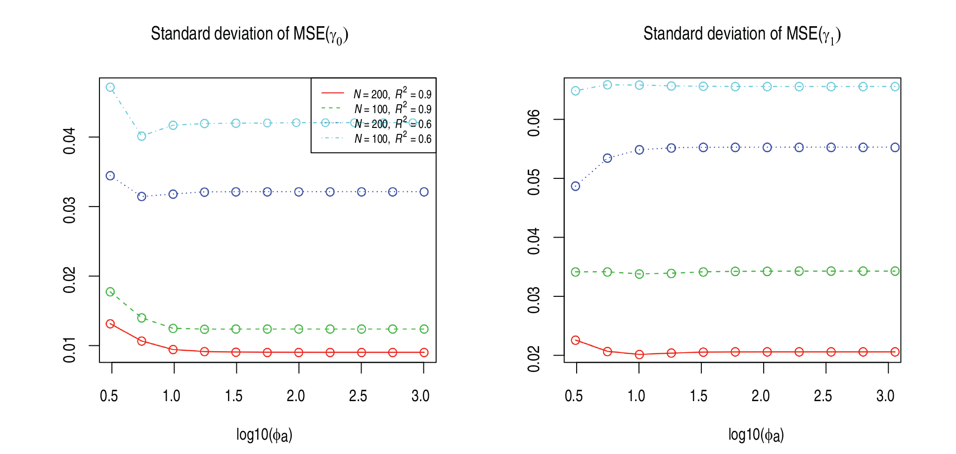
We have repeated the simulation for four scenarios: (a) , ; (b) , ; (c) , ; and (d) , . The prior information used to obtain LongPEER estimates of and is plotted in the top panel of Figure 5. Results for AIC, MSE and SSPE are displayed graphically in Figure 3. The standard deviation of MSE is plotted in Figure 4. As the sample size and increased, both MSE and MSE decreased, providing empirical evidence that the LongPEER estimates were consistent. In general, MSE() (except for ) and MSE() were minimized at and plateaued after that, that is, an increase in up to 10 resulted in improvement in estimation of both and and thereafter estimation performance remained almost unchanged. Finally, note that the value of that maximized AIC also minimized MSE and MSE. These results suggest that (a) AIC can be used to guide the choice of , and (b) with a sufficiently large ratio of , there is minimal impact on the estimation performance.
Average AIC, SSPE and MSE for simulations, as described in Section 5.2 over 100 simulations. At , average AIC were maximized and MSE() and MSE() were minimized. In general, average AIC increased with the increase in sample size and whereas SSPE, MSE() and MSE() decreased.
Standard deviation of MSE() and MSE() over 100 simulations, as described in Section 5.2. Both standard deviations decreased with increasing sample size and and minimized at and plateaued after that.
Average estimates of the components of regression functions for simulations, as described in Section 5.2 with and . Top panel: prior information used in LongPEER estimation. Middle and bottom panels: the average estimates of and ; these improve as and/or increase.
The average LongPEER estimates of and using a decomposition penalty are displayed in Figure 5, with and . For smaller sample sizes and , the LongPEER estimate may: (a) oversmooth (i.e., negatively bias) the estimated regression function at locations of a true feature and (b) be positively biased in locations corresponding to features in but the true is zero. However, by increasing the sample size to 200 and/or to 0.9, we observe that the average LongPEER estimates and approach the true functions.
Coverage probability
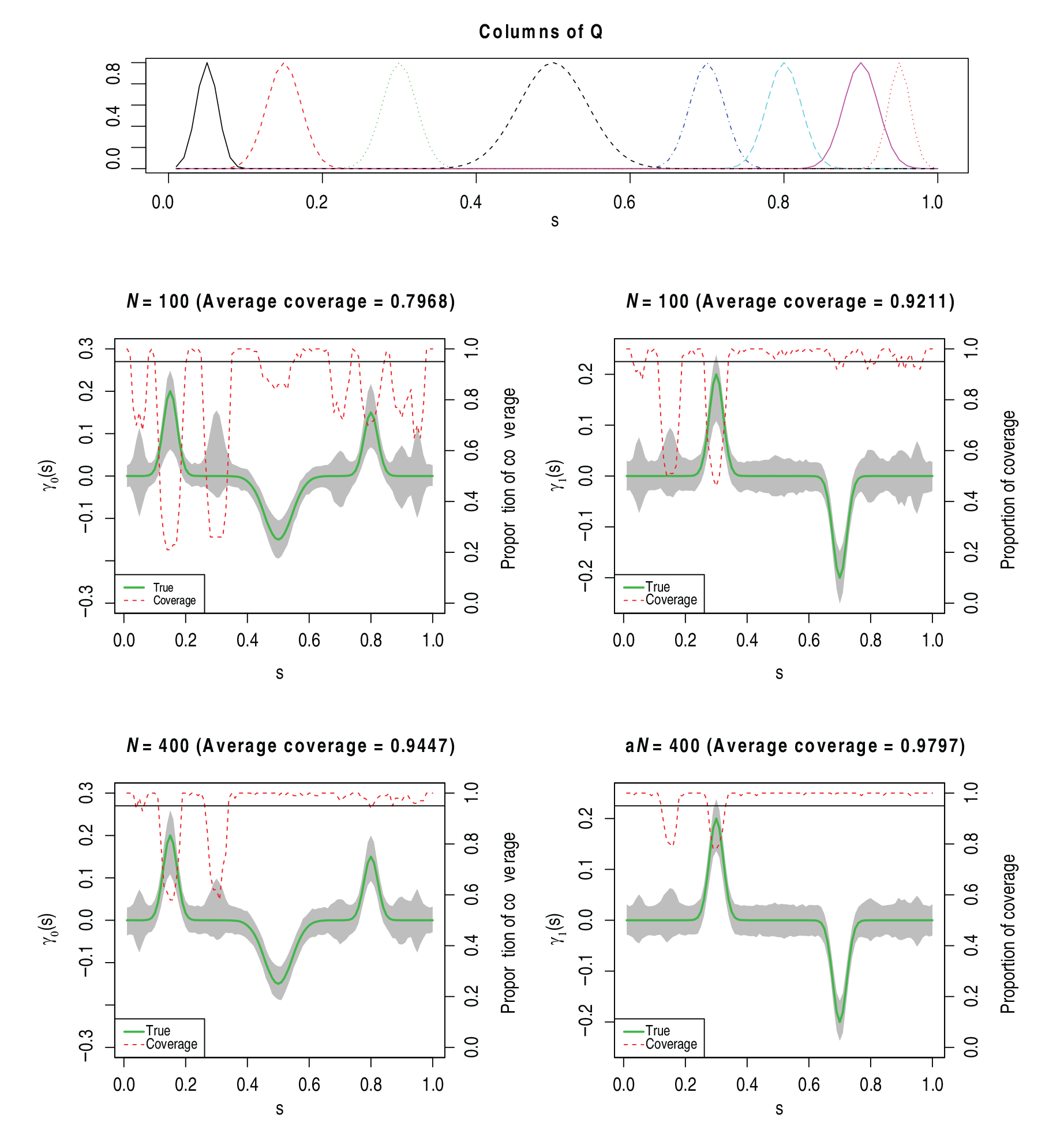
Coverage probabilities of LongPEER estimates in 100 simulations with and , as discussed in Section 5.3. Top panel: Prior information used in LongPEER estimation. Middle and bottom panels: 95% confidence band (shaded region) and coverage proportions (the dotted line) based on , and subjects, respectively. The left column displays the cross-sectional function and the right column displays the longitudinal function . The horizontal line in each plot marks the nominal coverage of 95%.
In this section, data were generated according to simulation scenario described in Section 5.2 with . The prior information used in LongPEER estimation along with the confidence bands and the coverage probabilities of LongPEER estimates are displayed in Figure 6. The 95% confidence bands are constructed as discussed in Section 4.2.
A notable improvement in coverage probabilities for both and was observed with the increase of . For , the coverage for both and was close to nominal level of 95%. We can see the dip in coverage probability in the first feature in at due to negative estimation bias (i.e., over-smoothing); however, the coverage probability improves when increases. We also explored the influence of on the confidence band and coverage probability (not shown here). The higher values of led to the confidence band shrinkage and this in turn resulted in under-coverage of both and .
Estimation in the presence of incomplete information
Top panel: true regression functions (solid lines) (left) and (right) and prior information about features (dashed lines). Note that there is no information about the peak at in . Middle panel: Average ridge penalty estimate from 100 simulations. Bottom panel: Average LongPEER estimate from 100 simulations using prior information is displayed in the top panel and .
Since the LongPEER estimate uses extrinsic scientific information in the estimation process, it is of interest to evaluate its estimation performance when only partial information is available. For this, we considered a simulation scenario similar to Section 5.3, but LongPEER estimate was obtained disregarding the information about the peak at . LongPEER estimates with (i.e., a ridge penalty) and , are displayed in Figure 7. LongPEER estimates of have an appropriate structure at , on average. Indeed as with an ordinary ridge penalty, this structure is inherited from the empirical eigenfunctions of . This highlights the advantage of an estimate obtained from the jointly determined eigenfunctions of and (see supplemental material available online in journal's website); the estimate depends on the relative contributions of predictor function and penalty (i.e., relative contribution of extrinsic information), controlled by . The relative increase in the contribution of extrinsic information resulted in shrinkage towards zero at in LongPEER estimate.
MRS study application
Prediction performance of model, as described in equation (6.1). Left panel: observed GDS score () and predicted value (). Right panel: observed and residuals .
We applied LongPEER to investigate potential associations of metabolite spectra, obtained from basal ganglia, and the global deficit score (GDS) in a longitudinal study of late-stage HIV patients. Of particular interest is how such an association evolves over time. The study cohort was comprised of chronically HIV-infected patients enrolled in the HIV Neuroimaging Consortium (HIVNC), a longitudinal study of HIV-associated brain injury, at multiple sites in the United States. At the time of enrolment, patients were on a stable anti-retroviral treatment. More detailed study description is available in Harezlak et al. (2011). We treat GDS as our scalar continuous response variable and MR spectrum (sampled at distinct frequencies) as functional predictor. GDS is often used as a continuous measure of neurocognitive impairment (e.g., Carey et al., 2004) and a large GDS score indicates a high degree of impairment. The MRS spectra are comprised of pure metabolite spectra, instrument noise and a background profile. We collected a total of observations from subjects. The longitudinal observations for each subject were within three years from baseline. The number of observations per subject ranged from 1 to 5 with a median equal to 3. Spectral information of following nine pure metabolites was used as prior information for the LongPEER estimation: Creatine (Cr), Glutamate (Glu), Glucose (Glc), Glycerophosphocholine (GPC), myo-Inositol (Ins), N-Acetylaspartate (NAA), N-Acetylaspartylglutamate (NAAG), scyllo-Inositol (Scyllo) and Taurine (Tau). These spectra are displayed in Figure 1.
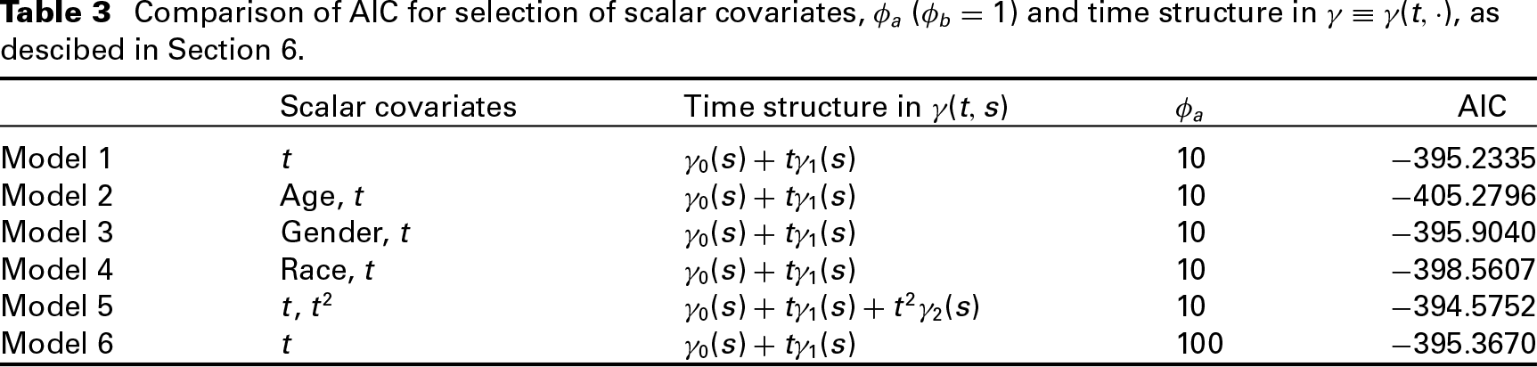
Information available on demographic factors includes: age at baseline, gender and race. We relied on AIC to choose (a) scalar covariates in the model, (b) (while setting ) for determining the relative contribution of prior information and (c) the time structure of . Based on the AIC (see Table 3), Models 1, 3, 5 and 6 are almost identical and appear to be better than the remaining models. In this illustration, we choose to consider relatively simple model. We fit Model 1 (with ,) as follows:
where . and are GDS and basal ganglia spectrum for subject at time , respectively. The LongPEER estimates were obtained as BLUP, assuming and the subject-specific random intercepts .
The estimates of (tuning parameter) associated with and were and , respectively, and the estimates of and were 0.0786 and 0.3332, respectively. The GDS score, fitted values and residual plot are displayed in Figure 8 for the purpose of model checking. The residuals do not show any obvious pattern.
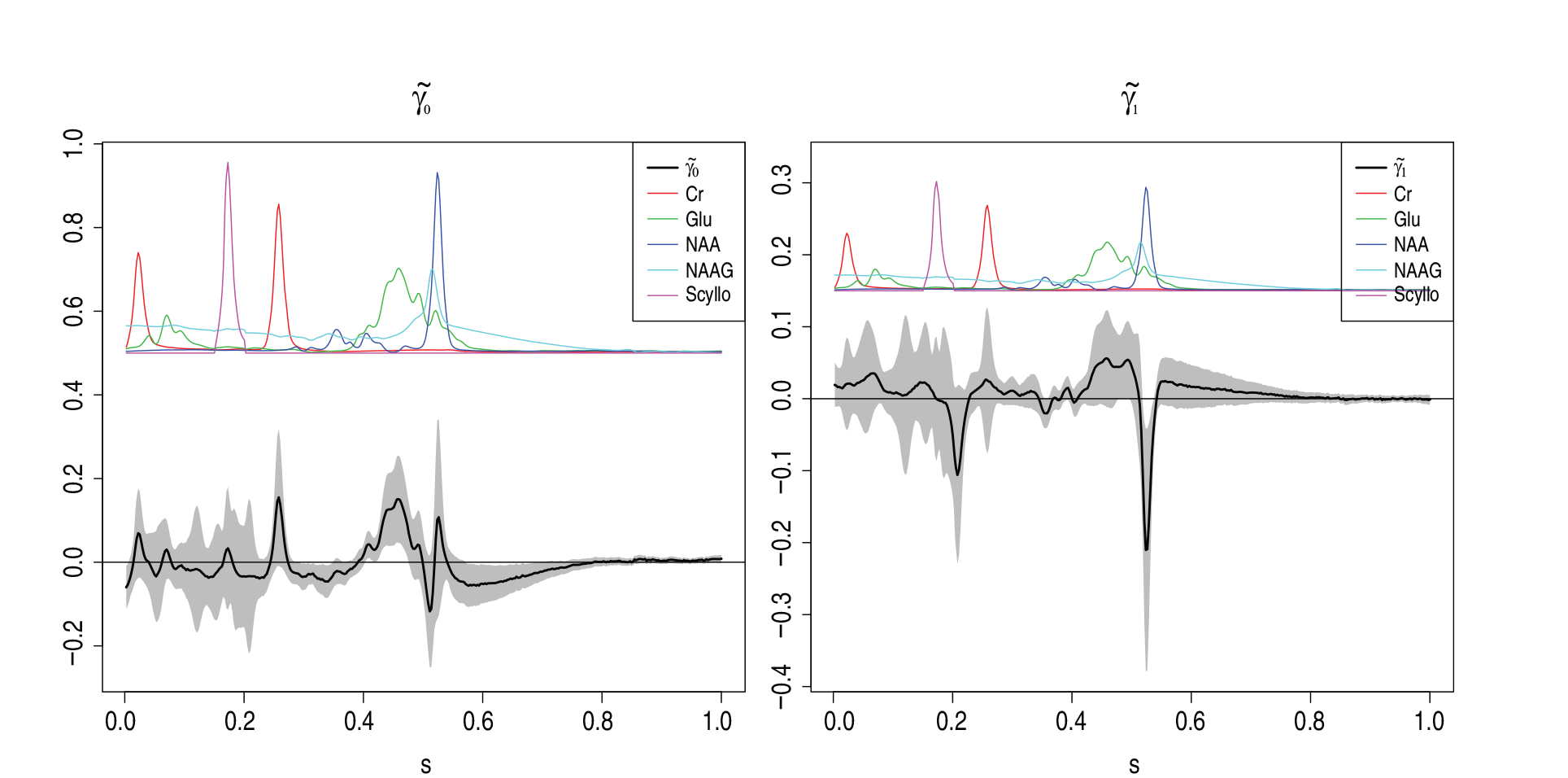
LongPEER estimates of and with , as described in Section 6. Shaded region in both the plots represent 95% pointwise confidence bands. Selected (scaled) pure metabolite spectra are also shown on both plots.
Comparison of AIC for selection of scalar covariates, () and time structure in , as descibed in Section 6.
Scalar covariates
Time structure in
AIC
Model 1
10
Model 2
Age,
10
Model 3
Gender,
10
Model 4
Race,
10
Model 5
,
10
Model 6
100
0
Figure 9 displays the estimates of and with pointwise 95% confidence bands. To aid interpretation, selected pure metabolite spectra are displayed. These figures reveal that estimated (the ‘baseline’ part of the regression function) is different from zero at the locations where at least one of the pure metabolites Cr, Glu, NAA, NAAG and Scyllo has a bump. Similarly, each non-zero part of estimated (the ‘longitudinal’ part of the regression function) coincides with bump locations of one or more pure metabolite profiles of Cr, Glu, NAA, GPC and Ins.
Pointwise confidence intervals for and contain the line over large intervals. The estimated is significant in the region and estimated is significant in a region . To be precise, peaks in both and are significant at locations where at least one of the pure metabolite profiles NAA or Glu have bumps. The observation of negative ‘longitudinal’ effect of NAA is worth commenting; it suggests that GDS increases as NAA concentration decreases in basal ganglia, a finding consistent with several studies in which a reduced concentration of NAA is seen to be associated with a decrease in neuronal mass (Christiansen et al., 1993; Lim and Spielman, 1997; Soares and Law, 2009).
Finally, we considered other forms of , such as or . However, relative improvement in AIC due to use of these complex structure was very minimal. For example, AIC associated with was observed as in comparison to AIC of observed with .
Discussion
We have proposed a novel estimation method for longitudinal functional regression and derived some properties of the estimated regression function. A valuable contribution of this framework is that it allows this estimate to vary with time as it extends the scope of penalized regression to the realm of longitudinal data. The approach may be viewed as an extension of longitudinal mixed effects models, replacing scalar predictors by functional predictors. Advantages of this framework include: estimating a time-dependent regression function, ability to incorporate structural information into the estimation process and easy implementation through linear mixed model equivalence.
The first simulation study of Section 5.1 illustrates the potential advantage of LongPEER estimate in exploiting an informed structured penalty, as compared to the more generic smoothness or spline-based constraints. The simulation in Section 5.3 suggests that coverage probabilities of the confidence bands for the true regression function are close to the nominal level. However, for small sample sizes, the naive confidence bands do not seem to be sufficient and an alternative solution that takes into account the estimation bias is needed. In the case when only partial information is available, the proposed method can be still useful, if we limit the relative contribution of the ‘informed’ space and/or increase the sample size (see Section 5.4). In the absence of prior information, one may impose more vaguely defined constraints—such as identity penalties, smoothing penalties or re-weighted projections onto empirical subspaces—to estimate the regression function.
Estimation in generalized ridge regression can be expressed in many forms. Clearly, one natural way to view this is via a Bayesian equivalence formulation (see, e.g., Robinson, 1991) with the informative priors quantifying the available scientific knowledge. In our formulation, the linear mixed model equivalence provides an easy computational implementation as well as an automatic choice of the tuning parameters using REML criterion. As detailed in the Supplemental material, GSVD provides intuition and insight about the role of the penalty operator via an explicit algebraic formulation of the estimate. Indeed, estimate of is obtained from a simultaneous diagonalization of and . The GSVD also provides explicit derivations of the bias and variance for the estimate.
A possible extension of this work is to incorporate multiple functional predictors. Consider we have two predictor functions and and the associated regression functions are and . Now, express and . Then the component functions can be estimated as BLUP from the mixed model: , where , and represent design matrices for the two functional predictors. Another possible extension is when response variable is binary or count. Indeed, an important problem that arises is to understand the neurocognitive impairment status of HIV patients, based on MRS collected over time. Estimation in these general settings appears to be possible with the proposed framework.
Footnotes
Acknowledgments
The authors wish to thank two anonymous referees and the associate editor for several corrections and suggestions that greatly improved the paper. The authors also extend their thank to Dr B. Navia who provided the MRS data used as an example in the manuscript. Partial research support was provided by the National Institutes of Health grants U01-MH083545 (JH), R01-MH108467 (JH), R01-CA126205 (TR) and U01-CA086368 (TR).
References
1.
BjorckA (1996) Numerical Methods for Least Square Problems, 1st edition. Philadelphia: SIAM.
2.
CaiTHallP (2006) Prediction in functional linear regression. The Annals of Statistics, 34, 2159–79.
3.
CardotHCrambesCKneipASardaP (2007) Smoothing splines estimators in functional linear regression with errors-in-variables. Computational Statistics Data Analysis, 51, 4832–48.
4.
CardotHFerratyFSardaP (2003) Spline estimators for the functional linear model. Statistica Sinica13, 571–91.
5.
CardotHCrambesCKneipASardaP (2007) Smoothing splines estimators in functional linear regression with errors-in-variables. Computational Statistics Data Analysis51, 4832–48.
6.
CareyCWoodsSGonzalezRConoverEMarcotteTGrantIHeatonR (2004) Predictive validity of global deficit scores in detecting neuropsychological impairment in HIV infection. Journal of Clinical and Experimental Neuropsychology, 26, 307–19.
7.
ChristiansenPToftPLarssonHStubgaardMHenriksenO (1993) The concentration of N-acetyl aspartate, creatine+phosphocreatine, and choline in different parts of the brain in adulthood and senium. Magnetic Resonance Imaging, 11, 799–806.
8.
CrainiceanuCReissPGoldsmithAHuangLHuoLScheiplF (2012) refund: Regression with Functional Data (R package version 0.1-6). Retrieved 11 January 2016, from http://CRAN.R-project.org/package=refund.
9.
EnglHWHankeMNeubauerA (2000) Regularization of Inverse Problems Vol. 375, Springer Science.
10.
FanJZhangJ (2000) Two-step estimation of functional linear models with applications to longitudinal data. Journal of the Royal Statistical Society: Series B (Statistical Methodology), 62, 303–22.
11.
FarawayJ (1997) Regression analysis for a functional response. Technometrics, 39, 254–61.
12.
FitzmauriceMLairdGWareJ (2004) Applied Longitudinal Analysis, 1st edition (Wiley Series in Probability and Statistics). John Wiley & Sons.
13.
GertheissJGoldsmithJCrainiceanuCGrevenS (2013) Longitudinal scalar-on-functions regression with application to tra- ctography data. Biostatistics, 14, 447–61.
14.
GoldsmithJBobbJCrainiceanuCCaffoBReichD (2011) Penalized functional regression. Journal of Computational and Graphical Statistics, 20, 830–51.
15.
GoldsmithJBobbJCrainiceanuCCaffoBReichD (2012) Longitudinal penalized functional regression for cognitive outcomes on neuronal tract measurements. Journal of the Royal Statistical Society: Series C, 61, 453–69.
16.
GrevenSCrainiceanuCCaffoBReichD (2011) Longitudinal functional principal component analysis. Recent Advances in Functional Data Analysis and Related Topics, 1st edition, pages 149–154. Physica-Verlag HD.
17.
HarezlakJBuchthalSTaylorMSchifittoGZhongJDaarEAlgerJSingerECampbellTYiannoutsosC (2011) Persistence of HIV-associated cognitive impairment, inflammation, and neuronal injury in era of highly active antiretroviral treatment. AIDS, 25, 625–33.
18.
HendersonC (1950) Estimation of genetic parameters (abstract). Annals of Mathematical Statistics, 21, 309–10.
JamesG (2002) Generalized linear models with functional predictors. Journal of the Royal Statistical Society: Series B (Statistical Methodology), 64, 411–32.
21.
LimKSpielmanD (1997) Estimating NAA in cortical gray matter with applications for measuring changes due to aging. Magnetic Resonance in Medicine, 37, 372–77.
22.
MorrisJCarrollR (2006) Wavelet-based functional mixed models. Journal of the Royal Statistical Society: Series B (Statistical Methodology), 68, 179–99.
23.
MüllerH (2005) Functional modelling and classification of longitudinal data. Scandinavian Journal of Statistics, 32, 223–40.
24.
MüllerHStadtmüllerU (2005) Generalized functional linear models. The Annals of Statistics, 33, 774–805.
25.
RamsayJDalzellC (1991) Some tools for functional data analysis. Journal of the Royal Statistical Society. Series B (Methodological), 53, 539–72.
26.
RamsayJSilvermanB (1997) Functional Data Analysis, 1st edition. Berlin: Springer-Verlag.
27.
RandolphTHarezlakJFengZ (2012) Structured penalties for functional linear models–partially empirical eigenvectors for regression. Electronic Journal of Statistics, 6, 323–53.
28.
ReissPOgdenR (2009) Smoothing parameter selection for a class of semiparametric linear models. Journal of the Royal Statistical Society: Series B (Stat Method), 71, 505–23.
29.
RobinsonG (1991) That blup is a good thing: The estimation of random effects. Statistical Science, 6, 15–32.
30.
RuppertDWandMCarrollR (2003) Semiparametric Regression, 1st edition. (Cambridge Series in Statistical and Probabilistic Mathematics). Cambridge University Press.
31.
SalganikMWandMLangeN (2004) Comparison of feature significance quantile approximations. Australian and New Zealand Journal of Statistics, 46, 569–81.
32.
SilvermanBW (1996) Smoothed functional principal components analysis by choice of norm. Annals of Statistics, 24, 1–24.
33.
SoaresDLawM (2009) Magnetic resonance spectroscopy of the brain: Review of metabolites and clinical applications. Clinical Radiology, 64, 12–21.
34.
TikhonovAN (1963) Solution of incorrectly formulated problems and the regularization method. Doklady Akademii Nauk SSSR, 151. 501–504 (in Russian); English transl.: Soviet Math. Dokl., 4, 1035–38.